EconML Tutorial 15: Common Pitfalls, Debugging, And Reporting

This final EconML tutorial is about failure modes. The earlier notebooks showed how to fit estimators, inspect heterogeneity, estimate policies, and build an end-to-end case study. Real applied causal work often fails in quieter ways: weak overlap, leakage, invalid controls, poor nuisance models, overfit CATE stories, or reports that hide key assumptions.

The notebook uses a synthetic observational setting with known truth. That lets us run a clean reference analysis and then deliberately contaminate the workflow in several ways. The goal is to learn what the failure modes look like in tables, figures, and policy outputs.

Learning Goals

By the end of this notebook, you should be able to:

Recognize when treatment overlap is weak enough to make CATE estimates fragile.
Detect leakage from outcome-like or post-treatment features.
Understand why bad nuisance models can distort average and heterogeneous effects.
See why conditioning on post-treatment variables can block part of the effect you want to estimate.
Avoid over-reading noisy unit-level CATE estimates.
Build a transparent reporting checklist for EconML analyses.

Notebook Flow

The workflow is diagnostic rather than estimator-first:

Build a clean teaching dataset with known treatment effects.
Fit a reference EconML model and save its diagnostics.
Stress-test overlap using propensity buckets and trimming logic.
Create a leakage example and show why it is invalid even when metrics look appealing.
Compare flexible nuisance models with overly simple nuisance models.
Show how post-treatment controls can change the estimand.
Use calibration, segments, and bootstrap intervals to avoid overconfident CATE stories.
End with a reusable debugging and reporting checklist.

Setup

The first code cell imports the libraries, configures plotting, suppresses known implementation warnings, and creates output folders. The MPLCONFIGDIR setting prevents Matplotlib cache warnings during notebook execution.

from pathlib import Path
import os
import time
import warnings

NOTEBOOK_DIR = Path.cwd()
if NOTEBOOK_DIR.name != "econml":
    NOTEBOOK_DIR = Path("notebooks/tutorials/econml").resolve()

OUTPUT_DIR = NOTEBOOK_DIR / "outputs"
FIGURE_DIR = OUTPUT_DIR / "figures"
TABLE_DIR = OUTPUT_DIR / "tables"
REPORT_DIR = OUTPUT_DIR / "reports"
for directory in [FIGURE_DIR, TABLE_DIR, REPORT_DIR, OUTPUT_DIR / "matplotlib_cache"]:
    directory.mkdir(parents=True, exist_ok=True)

os.environ.setdefault("MPLCONFIGDIR", str((OUTPUT_DIR / "matplotlib_cache").resolve()))

warnings.filterwarnings("ignore", category=FutureWarning)
warnings.filterwarnings("ignore", message=".*IProgress.*")
warnings.filterwarnings("ignore", message="X does not have valid feature names.*")
warnings.filterwarnings("ignore", message=".*column-vector y was passed.*")
warnings.filterwarnings("ignore", message=".*Co-variance matrix is underdetermined.*")
warnings.filterwarnings("ignore", message=".*lbfgs failed to converge.*")
warnings.filterwarnings("ignore", message=".*invalid value encountered.*")

import numpy as np
import pandas as pd
import seaborn as sns
import matplotlib.pyplot as plt
from IPython.display import display, Markdown
from scipy.special import expit
from sklearn.ensemble import RandomForestClassifier, RandomForestRegressor
from sklearn.linear_model import LinearRegression, LogisticRegression
from sklearn.metrics import log_loss, mean_absolute_error, mean_squared_error, r2_score, roc_auc_score
from sklearn.model_selection import train_test_split
from sklearn.preprocessing import PolynomialFeatures

from econml.dml import CausalForestDML, LinearDML
from econml.dr import DRLearner

sns.set_theme(style="whitegrid", context="notebook")
plt.rcParams["figure.dpi"] = 120
pd.set_option("display.max_columns", 100)
pd.set_option("display.float_format", lambda value: f"{value:,.4f}")

The environment is ready and all outputs will be written with a 15_ prefix. This keeps the final tutorial artifacts separate from earlier notebooks in the same folder.

Reproducibility Settings

The notebook uses simulation, train-test splits, tree models, and bootstrap resampling. The seed keeps results stable while preserving enough randomness to reveal realistic failure patterns.

RANDOM_STATE = 20260430
rng = np.random.default_rng(RANDOM_STATE)
CASE_PREFIX = "15"
N_USERS = 5_200
TEST_SIZE = 0.30
TREATMENT_COST = 0.16

settings = pd.DataFrame(
    {
        "setting": ["random_state", "n_users", "test_size", "treatment_cost"],
        "value": [RANDOM_STATE, N_USERS, TEST_SIZE, TREATMENT_COST],
        "why_it_matters": [
            "Makes the synthetic examples and bootstrap checks reproducible.",
            "Keeps estimator fitting fast while leaving enough rows for diagnostics.",
            "Creates held-out data for honest model comparison.",
            "Turns treatment effects into net decision value.",
        ],
    }
)
settings.to_csv(TABLE_DIR / f"{CASE_PREFIX}_analysis_settings.csv", index=False)
display(settings)

	setting	value	why_it_matters
0	random_state	20,260,430.0000	Makes the synthetic examples and bootstrap che...
1	n_users	5,200.0000	Keeps estimator fitting fast while leaving eno...
2	test_size	0.3000	Creates held-out data for honest model compari...
3	treatment_cost	0.1600	Turns treatment effects into net decision value.

The cost value will be used later to show why good CATE estimates are not enough. A policy must create net value after costs, not merely produce positive estimated effects.

Pitfall Map

Before touching data, we write down the specific risks this notebook will demonstrate. This habit helps separate causal design problems from software or modeling problems.

pitfall_map = pd.DataFrame(
    [
        ("Weak overlap", "Some users have almost no chance of being treated or untreated.", "Propensity distributions, bucket counts, effective sample size, trimming checks."),
        ("Outcome leakage", "A feature contains future outcome information or is built after the outcome window.", "Too-good metrics, suspicious feature timing, impossible prediction inputs."),
        ("Post-treatment controls", "A mediator or downstream variable is used as a confounder.", "Estimated effect changes because part of the treatment pathway is blocked."),
        ("Bad nuisance models", "Treatment or outcome models are too weak for the adjustment problem.", "Poor nuisance diagnostics, unstable CATE estimates, weak calibration."),
        ("Overread unit CATE", "Individual treatment effects are treated as precise facts.", "Noisy scatter, unstable deciles, wide bootstrap policy intervals."),
        ("Segment hunting", "Many segments are searched until some look impressive by chance.", "Random segment stress tests and transparent multiple-comparison caveats."),
        ("Thin reporting", "A report gives a point estimate without assumptions, diagnostics, or caveats.", "Checklist requiring estimand, overlap, model diagnostics, sensitivity, and decision context."),
    ],
    columns=["risk", "what_goes_wrong", "how_to_debug"],
)
pitfall_map.to_csv(TABLE_DIR / f"{CASE_PREFIX}_pitfall_map.csv", index=False)
display(pitfall_map)

	risk	what_goes_wrong	how_to_debug
0	Weak overlap	Some users have almost no chance of being trea...	Propensity distributions, bucket counts, effec...
1	Outcome leakage	A feature contains future outcome information ...	Too-good metrics, suspicious feature timing, i...
2	Post-treatment controls	A mediator or downstream variable is used as a...	Estimated effect changes because part of the t...
3	Bad nuisance models	Treatment or outcome models are too weak for t...	Poor nuisance diagnostics, unstable CATE estim...
4	Overread unit CATE	Individual treatment effects are treated as pr...	Noisy scatter, unstable deciles, wide bootstra...
5	Segment hunting	Many segments are searched until some look imp...	Random segment stress tests and transparent mu...
6	Thin reporting	A report gives a point estimate without assump...	Checklist requiring estimand, overlap, model d...

The rest of the notebook turns these rows into concrete examples. The point is not that EconML is fragile; the point is that causal estimation is only as credible as the design and diagnostics around it.

Synthetic Data-Generating Process

The helper functions define a clean target causal problem. We create pre-treatment user features, a treatment assignment mechanism, a baseline outcome, and a true heterogeneous treatment effect.

The simulation also creates two dangerous columns: a post-treatment activity variable and a leaky outcome proxy. They are intentionally included so we can demonstrate why they should not be used as normal pre-treatment features.

def make_correlated_normals(n_rows, n_features, correlation, rng):
    covariance = np.full((n_features, n_features), correlation)
    np.fill_diagonal(covariance, 1.0)
    return rng.multivariate_normal(np.zeros(n_features), covariance, size=n_rows)


def true_cate_function(frame):
    return (
        0.24
        + 0.30 * frame["need_score"]
        + 0.22 * frame["preference_match"]
        + 0.16 * np.maximum(frame["search_friction"], 0)
        - 0.20 * frame["price_sensitivity"]
        + 0.14 * frame["high_intent_segment"]
        + 0.08 * frame["device_quality"] * frame["preference_match"]
        - 0.10 * frame["competitive_pressure"]
    )


def treatment_propensity_function(frame, severe=False):
    multiplier = 1.8 if severe else 1.0
    logit = multiplier * (
        -0.15
        + 0.62 * frame["need_score"]
        + 0.50 * frame["prior_activity"]
        + 0.40 * frame["high_intent_segment"]
        + 0.35 * frame["marketing_intensity"]
        - 0.30 * frame["device_quality"]
        + 0.20 * frame["search_friction"]
    )
    lower, upper = (0.01, 0.99) if severe else (0.05, 0.95)
    return np.clip(expit(logit), lower, upper)


def baseline_outcome_function(frame):
    return (
        1.20
        + 0.48 * frame["prior_activity"]
        + 0.36 * frame["preference_match"]
        - 0.34 * frame["search_friction"]
        - 0.22 * frame["price_sensitivity"]
        + 0.24 * frame["device_quality"]
        + 0.16 * frame["market_maturity"]
        + 0.12 * frame["organic_source"]
        + 0.06 * np.sin(frame["tenure_weeks"] / 4.0)
    )

The true CATE is deliberately nonlinear. That makes the clean analysis nontrivial and gives us a useful benchmark when we later compare bad design choices.

Generate The Teaching Dataset

This cell creates an observational user table. Treatment is targeted, the outcome is noisy, and a few fields have light missingness. The dangerous fields are clearly named so their timing problems are visible.

latent = make_correlated_normals(N_USERS, 6, correlation=0.25, rng=rng)
data = pd.DataFrame(
    {
        "user_id": np.arange(1, N_USERS + 1),
        "need_score": latent[:, 0],
        "prior_activity": latent[:, 1],
        "preference_match": latent[:, 2],
        "search_friction": latent[:, 3],
        "price_sensitivity": latent[:, 4],
        "device_quality": latent[:, 5],
    }
)

data["marketing_intensity"] = rng.normal(0, 1, N_USERS)
data["competitive_pressure"] = rng.normal(0, 1, N_USERS)
data["market_maturity"] = rng.normal(0, 1, N_USERS)
data["tenure_weeks"] = np.clip(rng.gamma(shape=3.0, scale=4.0, size=N_USERS), 1, 48)
data["organic_source"] = rng.binomial(1, expit(0.10 + 0.30 * data["preference_match"]), N_USERS)
data["weekday_signup"] = rng.binomial(1, 0.70, N_USERS)
data["high_intent_segment"] = rng.binomial(
    1,
    expit(0.35 * data["prior_activity"] + 0.30 * data["preference_match"] - 0.12 * data["price_sensitivity"]),
    N_USERS,
)

data["true_cate"] = true_cate_function(data)
data["true_propensity"] = treatment_propensity_function(data, severe=False)
data["treatment"] = rng.binomial(1, data["true_propensity"], N_USERS)
data["baseline_outcome"] = baseline_outcome_function(data)
data["outcome"] = data["baseline_outcome"] + data["treatment"] * data["true_cate"] + rng.normal(0, 0.70, N_USERS)

# These two columns are intentionally dangerous. They are not valid pre-treatment controls.
data["post_treatment_activity"] = 0.65 * data["treatment"] + 0.40 * data["true_cate"] + 0.35 * data["prior_activity"] + rng.normal(0, 0.55, N_USERS)
data["leaky_outcome_proxy"] = data["outcome"] + rng.normal(0, 0.20, N_USERS)

for column, missing_rate in {"preference_match": 0.025, "search_friction": 0.030, "device_quality": 0.020}.items():
    data.loc[rng.random(N_USERS) < missing_rate, column] = np.nan

data.to_csv(TABLE_DIR / f"{CASE_PREFIX}_pitfall_teaching_data.csv", index=False)
display(data.head())

	user_id	need_score	prior_activity	preference_match	search_friction	price_sensitivity	device_quality	marketing_intensity	competitive_pressure	market_maturity	tenure_weeks	organic_source	weekday_signup	high_intent_segment	true_cate	true_propensity	treatment	baseline_outcome	outcome	post_treatment_activity	leaky_outcome_proxy
0	1	0.7059	0.0571	-0.5594	0.8454	0.1722	1.0620	0.8506	0.0623	-1.1204	11.2538	1	1	0	0.3758	0.6141	1	0.9157	0.2184	0.6957	0.0188
1	2	-0.0540	-0.2884	0.9522	0.2782	-1.7934	0.2560	-2.0918	0.5260	1.8166	9.3135	1	0	1	0.9434	0.3360	0	2.2200	2.4476	0.9286	2.3796
2	3	1.8433	0.4595	0.9130	1.0479	0.3843	0.2413	-0.6062	-1.2137	1.0250	24.2055	1	1	1	1.3636	0.8246	0	1.6365	1.3172	1.5100	1.2147
3	4	0.0350	0.1052	1.4770	0.3775	-1.7736	1.2076	0.0720	-1.5952	-1.3030	8.5236	1	0	1	1.4328	0.5157	0	2.2962	3.0734	-0.2245	3.1225
4	5	0.2625	1.3947	0.1096	-0.5099	-1.4671	-1.2981	1.2255	-1.7827	-0.4524	12.2572	0	1	1	0.9432	0.8613	1	2.0258	1.8911	1.3667	1.8260

The dataset includes the clean ingredients plus two traps. post_treatment_activity happens after treatment and may mediate the treatment effect. leaky_outcome_proxy is essentially future outcome information. Both would make a real CATE analysis invalid if used as normal covariates.

Field Dictionary And Timing Audit

A timing audit is one of the best leakage defenses. Every feature should be labeled as pre-treatment, treatment, outcome, post-treatment, or hidden teaching truth.

field_dictionary = pd.DataFrame(
    [
        ("user_id", "Identifier", "Row identifier.", "Identifier", "Do not model."),
        ("need_score", "Numeric", "Pre-treatment signal of onboarding need.", "Pre-treatment", "Allowed X."),
        ("prior_activity", "Numeric", "Pre-treatment usage activity.", "Pre-treatment", "Allowed X."),
        ("preference_match", "Numeric", "Pre-treatment match between user interests and catalog.", "Pre-treatment", "Allowed X."),
        ("search_friction", "Numeric", "Pre-treatment difficulty finding relevant content.", "Pre-treatment", "Allowed X."),
        ("price_sensitivity", "Numeric", "Pre-treatment cost sensitivity proxy.", "Pre-treatment", "Allowed X."),
        ("device_quality", "Numeric", "Pre-treatment device or experience quality proxy.", "Pre-treatment", "Allowed X."),
        ("high_intent_segment", "Binary", "Pre-treatment segment flag.", "Pre-treatment", "Allowed X."),
        ("marketing_intensity", "Numeric", "Other pre-treatment marketing pressure.", "Pre-treatment", "Allowed W."),
        ("competitive_pressure", "Numeric", "Pre-treatment market competition proxy.", "Pre-treatment", "Allowed W."),
        ("market_maturity", "Numeric", "Market maturity proxy.", "Pre-treatment", "Allowed W."),
        ("tenure_weeks", "Numeric", "Account age before treatment.", "Pre-treatment", "Allowed W."),
        ("organic_source", "Binary", "Acquisition source before treatment.", "Pre-treatment", "Allowed W."),
        ("weekday_signup", "Binary", "Signup timing before treatment.", "Pre-treatment", "Allowed W."),
        ("treatment", "Binary", "Whether the user received the intervention.", "Treatment", "T."),
        ("outcome", "Numeric", "Post-treatment outcome.", "Outcome", "Y."),
        ("post_treatment_activity", "Numeric", "Activity after treatment starts.", "Post-treatment", "Pitfall: do not adjust as a confounder."),
        ("leaky_outcome_proxy", "Numeric", "Noisy copy of the outcome.", "Outcome-like leakage", "Pitfall: do not use as a feature."),
        ("true_cate", "Numeric", "Known individual effect in simulation.", "Hidden truth", "Evaluation only."),
        ("true_propensity", "Numeric", "Known assignment probability in simulation.", "Hidden truth", "Evaluation only."),
        ("baseline_outcome", "Numeric", "Known untreated outcome component.", "Hidden truth", "Evaluation only."),
    ],
    columns=["field", "type", "description", "timing", "modeling_status"],
)
field_dictionary.to_csv(TABLE_DIR / f"{CASE_PREFIX}_field_dictionary_timing_audit.csv", index=False)
display(field_dictionary)

	field	type	description	timing	modeling_status
0	user_id	Identifier	Row identifier.	Identifier	Do not model.
1	need_score	Numeric	Pre-treatment signal of onboarding need.	Pre-treatment	Allowed X.
2	prior_activity	Numeric	Pre-treatment usage activity.	Pre-treatment	Allowed X.
3	preference_match	Numeric	Pre-treatment match between user interests and...	Pre-treatment	Allowed X.
4	search_friction	Numeric	Pre-treatment difficulty finding relevant cont...	Pre-treatment	Allowed X.
5	price_sensitivity	Numeric	Pre-treatment cost sensitivity proxy.	Pre-treatment	Allowed X.
6	device_quality	Numeric	Pre-treatment device or experience quality proxy.	Pre-treatment	Allowed X.
7	high_intent_segment	Binary	Pre-treatment segment flag.	Pre-treatment	Allowed X.
8	marketing_intensity	Numeric	Other pre-treatment marketing pressure.	Pre-treatment	Allowed W.
9	competitive_pressure	Numeric	Pre-treatment market competition proxy.	Pre-treatment	Allowed W.
10	market_maturity	Numeric	Market maturity proxy.	Pre-treatment	Allowed W.
11	tenure_weeks	Numeric	Account age before treatment.	Pre-treatment	Allowed W.
12	organic_source	Binary	Acquisition source before treatment.	Pre-treatment	Allowed W.
13	weekday_signup	Binary	Signup timing before treatment.	Pre-treatment	Allowed W.
14	treatment	Binary	Whether the user received the intervention.	Treatment	T.
15	outcome	Numeric	Post-treatment outcome.	Outcome	Y.
16	post_treatment_activity	Numeric	Activity after treatment starts.	Post-treatment	Pitfall: do not adjust as a confounder.
17	leaky_outcome_proxy	Numeric	Noisy copy of the outcome.	Outcome-like leakage	Pitfall: do not use as a feature.
18	true_cate	Numeric	Known individual effect in simulation.	Hidden truth	Evaluation only.
19	true_propensity	Numeric	Known assignment probability in simulation.	Hidden truth	Evaluation only.
20	baseline_outcome	Numeric	Known untreated outcome component.	Hidden truth	Evaluation only.

The timing audit is a simple but powerful debugging tool. Many impressive-looking causal models fail because a feature quietly includes information that would not exist at decision time.

Basic Data Quality Checks

Before fitting estimators, we confirm sample size, treatment share, outcome completeness, and missingness patterns.

basic_summary = pd.DataFrame(
    {
        "metric": ["rows", "columns", "treatment_rate", "outcome_missing", "treatment_missing", "true_ate"],
        "value": [
            len(data),
            data.shape[1],
            data["treatment"].mean(),
            data["outcome"].isna().sum(),
            data["treatment"].isna().sum(),
            data["true_cate"].mean(),
        ],
    }
)
missing_summary = (
    data.isna().mean().rename("missing_rate").reset_index().rename(columns={"index": "field"})
    .query("missing_rate > 0")
    .sort_values("missing_rate", ascending=False)
)
basic_summary.to_csv(TABLE_DIR / f"{CASE_PREFIX}_basic_summary.csv", index=False)
missing_summary.to_csv(TABLE_DIR / f"{CASE_PREFIX}_missing_summary.csv", index=False)
display(basic_summary)
display(missing_summary)

	metric	value
0	rows	5,200.0000
1	columns	21.0000
2	treatment_rate	0.5148
3	outcome_missing	0.0000
4	treatment_missing	0.0000
5	true_ate	0.3825

	field	missing_rate
4	search_friction	0.0290
3	preference_match	0.0242
6	device_quality	0.0221

The core treatment and outcome fields are complete. Light missingness appears only in pre-treatment features, which can be handled with train-only imputation.

Raw Outcome Gap

A raw treated-control comparison is not a causal estimate here, but it is still useful as a baseline. If it differs sharply from the true ATE, that is evidence that confounding matters.

raw_group_summary = (
    data.groupby("treatment")
    .agg(
        users=("user_id", "size"),
        mean_outcome=("outcome", "mean"),
        mean_true_cate=("true_cate", "mean"),
        mean_true_propensity=("true_propensity", "mean"),
    )
    .reset_index()
)
raw_gap = raw_group_summary.loc[raw_group_summary["treatment"] == 1, "mean_outcome"].iloc[0] - raw_group_summary.loc[raw_group_summary["treatment"] == 0, "mean_outcome"].iloc[0]
raw_gap_table = pd.DataFrame(
    {
        "quantity": ["raw_treated_minus_control", "true_ate", "raw_minus_true_ate"],
        "value": [raw_gap, data["true_cate"].mean(), raw_gap - data["true_cate"].mean()],
    }
)
raw_group_summary.to_csv(TABLE_DIR / f"{CASE_PREFIX}_raw_group_summary.csv", index=False)
raw_gap_table.to_csv(TABLE_DIR / f"{CASE_PREFIX}_raw_gap_vs_truth.csv", index=False)
display(raw_group_summary)
display(raw_gap_table)

	treatment	users	mean_outcome	mean_true_cate	mean_true_propensity
0	0	2523	1.1829	0.2605	0.4183
1	1	2677	1.8945	0.4974	0.6004

	quantity	value
0	raw_treated_minus_control	0.7116
1	true_ate	0.3825
2	raw_minus_true_ate	0.3292

The raw difference mixes selection and treatment impact. The treated group has a different average treatment propensity, so adjustment is necessary before making causal claims.

True CATE Distribution

The hidden true CATE distribution gives us the benchmark for later model checks. In real work, this distribution would be unknown.

true_cate_summary = data["true_cate"].describe(percentiles=[0.05, 0.25, 0.50, 0.75, 0.95]).to_frame("true_cate")
true_cate_summary.to_csv(TABLE_DIR / f"{CASE_PREFIX}_true_cate_summary.csv")

fig, ax = plt.subplots(figsize=(9, 5))
sns.histplot(data["true_cate"], bins=45, kde=True, color="#2563eb", ax=ax)
ax.axvline(TREATMENT_COST, color="#dc2626", linestyle="--", linewidth=1.5, label=f"Cost = {TREATMENT_COST:.2f}")
ax.axvline(data["true_cate"].mean(), color="#111827", linewidth=1.3, label="True ATE")
ax.set_title("Hidden True CATE Distribution")
ax.set_xlabel("True CATE")
ax.set_ylabel("Users")
ax.legend()
plt.tight_layout()
fig.savefig(FIGURE_DIR / f"{CASE_PREFIX}_true_cate_distribution.png", dpi=160, bbox_inches="tight")
plt.show()

display(true_cate_summary)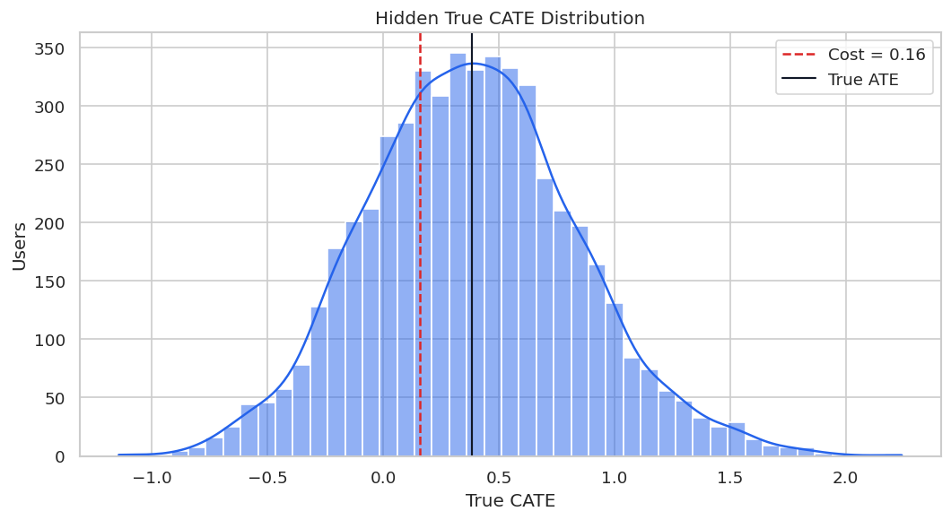

	true_cate
count	5,200.0000
mean	0.3825
std	0.4564
min	-1.1440
5%	-0.3367
25%	0.0684
50%	0.3722
75%	0.6712
95%	1.1626
max	2.2424

The spread in true CATE creates a legitimate targeting problem. The risk is that bad workflows can create a convincing but wrong story about that heterogeneity.

Define Clean Feature Roles

This is the clean design we want to protect. X contains pre-treatment effect modifiers, while W contains additional pre-treatment controls. Dangerous post-treatment and outcome-like fields are excluded.

CLEAN_X_COLUMNS = [
    "need_score",
    "prior_activity",
    "preference_match",
    "search_friction",
    "price_sensitivity",
    "device_quality",
    "high_intent_segment",
]
CLEAN_W_COLUMNS = [
    "marketing_intensity",
    "competitive_pressure",
    "market_maturity",
    "tenure_weeks",
    "organic_source",
    "weekday_signup",
]

feature_role_table = pd.DataFrame(
    {
        "field": CLEAN_X_COLUMNS + CLEAN_W_COLUMNS,
        "role": ["X"] * len(CLEAN_X_COLUMNS) + ["W"] * len(CLEAN_W_COLUMNS),
        "timing": "Pre-treatment",
    }
)
feature_role_table.to_csv(TABLE_DIR / f"{CASE_PREFIX}_clean_feature_roles.csv", index=False)
display(feature_role_table)

	field	role	timing
0	need_score	X	Pre-treatment
1	prior_activity	X	Pre-treatment
2	preference_match	X	Pre-treatment
3	search_friction	X	Pre-treatment
4	price_sensitivity	X	Pre-treatment
5	device_quality	X	Pre-treatment
6	high_intent_segment	X	Pre-treatment
7	marketing_intensity	W	Pre-treatment
8	competitive_pressure	W	Pre-treatment
9	market_maturity	W	Pre-treatment
10	tenure_weeks	W	Pre-treatment
11	organic_source	W	Pre-treatment
12	weekday_signup	W	Pre-treatment

The clean roles intentionally keep the CATE surface focused and exclude future information. Later pitfall examples will violate this design to show what can go wrong.

Train-Test Split

We split once and reuse the same rows across the clean analysis and pitfall examples. This makes comparisons easier to interpret.

train_df, test_df = train_test_split(
    data,
    test_size=TEST_SIZE,
    random_state=RANDOM_STATE,
    stratify=data["treatment"],
)
train_df = train_df.reset_index(drop=True)
test_df = test_df.reset_index(drop=True)

split_summary = pd.DataFrame(
    {
        "split": ["train", "test"],
        "rows": [len(train_df), len(test_df)],
        "treatment_rate": [train_df["treatment"].mean(), test_df["treatment"].mean()],
        "mean_outcome": [train_df["outcome"].mean(), test_df["outcome"].mean()],
        "mean_true_cate": [train_df["true_cate"].mean(), test_df["true_cate"].mean()],
    }
)
split_summary.to_csv(TABLE_DIR / f"{CASE_PREFIX}_train_test_split_summary.csv", index=False)
display(split_summary)

	split	rows	treatment_rate	mean_outcome	mean_true_cate
0	train	3640	0.5148	1.5562	0.3868
1	test	1560	0.5147	1.5332	0.3723

The train and test samples have similar treatment rates and average true effects. Reusing this split keeps the rest of the notebook apples-to-apples.

Matrix Builder

This helper prepares X, W, T, and Y matrices. It learns medians from the training data and can optionally add missingness flags to W.

def build_design(train_frame, test_frame, x_columns, w_columns, add_missing_flags=True):
    model_columns = list(dict.fromkeys(x_columns + w_columns))
    train_medians = train_frame[model_columns].median(numeric_only=True)
    missing_columns = [column for column in model_columns if train_frame[column].isna().any() or test_frame[column].isna().any()]

    def transform(frame):
        raw = frame[model_columns].copy()
        filled = raw.fillna(train_medians)
        X = filled[x_columns].astype(float)
        W = filled[w_columns].astype(float)
        if add_missing_flags and missing_columns:
            flags = raw[missing_columns].isna().astype(float).add_suffix("_missing")
            W = pd.concat([W, flags], axis=1)
        return X, W

    X_train, W_train = transform(train_frame)
    X_test, W_test = transform(test_frame)
    T_train = train_frame["treatment"].astype(int)
    T_test = test_frame["treatment"].astype(int)
    Y_train = train_frame["outcome"].astype(float)
    Y_test = test_frame["outcome"].astype(float)
    return X_train, W_train, T_train, Y_train, X_test, W_test, T_test, Y_test

X_train, W_train, T_train, Y_train, X_test, W_test, T_test, Y_test = build_design(
    train_df,
    test_df,
    CLEAN_X_COLUMNS,
    CLEAN_W_COLUMNS,
)
true_tau_test = test_df["true_cate"].to_numpy()

matrix_summary = pd.DataFrame(
    {
        "matrix": ["X_train", "W_train", "X_test", "W_test"],
        "rows": [X_train.shape[0], W_train.shape[0], X_test.shape[0], W_test.shape[0]],
        "columns": [X_train.shape[1], W_train.shape[1], X_test.shape[1], W_test.shape[1]],
        "missing_after_preparation": [
            int(X_train.isna().sum().sum()),
            int(W_train.isna().sum().sum()),
            int(X_test.isna().sum().sum()),
            int(W_test.isna().sum().sum()),
        ],
    }
)
matrix_summary.to_csv(TABLE_DIR / f"{CASE_PREFIX}_clean_matrix_summary.csv", index=False)
display(matrix_summary)

	matrix	rows	columns
0	X_train	3640	7
1	W_train	3640	9
2	X_test	1560	7
3	W_test	1560	9

The prepared matrices are complete and use only pre-treatment fields. This is the reference design against which the failure modes will be compared.

Reusable Model Helpers

These helper functions keep estimator setup consistent across examples. They also make the later comparison tables easier to read.

def make_rf_classifier(seed_offset=0, min_leaf=30):
    return RandomForestClassifier(
        n_estimators=160,
        min_samples_leaf=min_leaf,
        max_features=0.75,
        random_state=RANDOM_STATE + seed_offset,
        n_jobs=-1,
    )


def make_rf_regressor(seed_offset=0, min_leaf=25):
    return RandomForestRegressor(
        n_estimators=160,
        min_samples_leaf=min_leaf,
        max_features=0.75,
        random_state=RANDOM_STATE + seed_offset,
        n_jobs=-1,
    )


def safe_corr(left, right):
    if np.std(left) == 0 or np.std(right) == 0:
        return np.nan
    return float(np.corrcoef(left, right)[0, 1])


def summarize_effects(label, estimated, true_tau, fit_seconds, notes):
    estimated = np.asarray(estimated)
    top_mask = estimated >= np.quantile(estimated, 0.80)
    action = estimated > TREATMENT_COST
    return {
        "analysis": label,
        "estimated_ate": estimated.mean(),
        "true_ate_test": true_tau.mean(),
        "ate_bias": estimated.mean() - true_tau.mean(),
        "cate_rmse": mean_squared_error(true_tau, estimated) ** 0.5,
        "cate_mae": mean_absolute_error(true_tau, estimated),
        "cate_correlation": safe_corr(true_tau, estimated),
        "top_20_true_cate_mean": true_tau[top_mask].mean(),
        "share_estimated_above_cost": action.mean(),
        "true_net_policy_value": ((true_tau - TREATMENT_COST) * action).mean(),
        "fit_seconds": fit_seconds,
        "notes": notes,
    }

The summary function includes both estimation metrics and policy metrics. This is deliberate: a model can look acceptable statistically while still creating a weak decision rule.

Clean Reference Estimators

We begin with a reasonably careful reference analysis using only valid pre-treatment features. Two estimators are fit: a flexible causal forest and a doubly robust learner.

reference_estimators = {
    "Clean CausalForestDML": CausalForestDML(
        model_y=make_rf_regressor(101),
        model_t=make_rf_classifier(102),
        discrete_treatment=True,
        n_estimators=160,
        min_samples_leaf=18,
        max_samples=0.45,
        cv=3,
        random_state=RANDOM_STATE,
    ),
    "Clean DRLearner": DRLearner(
        model_propensity=make_rf_classifier(201),
        model_regression=make_rf_regressor(202),
        model_final=make_rf_regressor(203),
        min_propensity=0.02,
        cv=3,
        random_state=RANDOM_STATE,
    ),
}

reference_effects = {}
reference_rows = []
for label, estimator in reference_estimators.items():
    start = time.perf_counter()
    estimator.fit(Y_train, T_train, X=X_train, W=W_train)
    fit_seconds = time.perf_counter() - start
    estimated = estimator.effect(X_test)
    reference_effects[label] = estimated
    reference_rows.append(summarize_effects(label, estimated, true_tau_test, fit_seconds, "Clean pre-treatment design."))

reference_metrics = pd.DataFrame(reference_rows).sort_values("cate_rmse")
reference_metrics.to_csv(TABLE_DIR / f"{CASE_PREFIX}_reference_estimator_metrics.csv", index=False)
display(reference_metrics)

	analysis	estimated_ate	true_ate_test	ate_bias	cate_rmse	cate_mae	cate_correlation	top_20_true_cate_mean	share_estimated_above_cost	true_net_policy_value	fit_seconds	notes
1	Clean DRLearner	0.3458	0.3723	-0.0266	0.2532	0.1999	0.8484	0.9207	0.6365	0.2813	3.5359	Clean pre-treatment design.
0	Clean CausalForestDML	0.3609	0.3723	-0.0115	0.2667	0.2074	0.8733	0.9467	0.7494	0.2815	3.6758	Clean pre-treatment design.

The reference estimates are not perfect, but they give us a defensible baseline. Later tables will compare questionable workflows to these clean estimates.

Reference CATE Recovery Plot

The scatterplot compares the best clean reference estimator with the known true CATE. This visual is a useful reminder that individual CATEs are noisy even in a clean simulation.

best_reference_label = reference_metrics.iloc[0]["analysis"]
best_reference_effect = reference_effects[best_reference_label]

fig, ax = plt.subplots(figsize=(6.5, 6))
sns.scatterplot(x=true_tau_test, y=best_reference_effect, alpha=0.30, s=22, color="#2563eb", ax=ax)
min_value = min(true_tau_test.min(), best_reference_effect.min())
max_value = max(true_tau_test.max(), best_reference_effect.max())
ax.plot([min_value, max_value], [min_value, max_value], color="#dc2626", linestyle="--", linewidth=1.2)
ax.set_title(f"Reference CATE Recovery: {best_reference_label}")
ax.set_xlabel("True CATE")
ax.set_ylabel("Estimated CATE")
plt.tight_layout()
fig.savefig(FIGURE_DIR / f"{CASE_PREFIX}_reference_cate_recovery.png", dpi=160, bbox_inches="tight")
plt.show()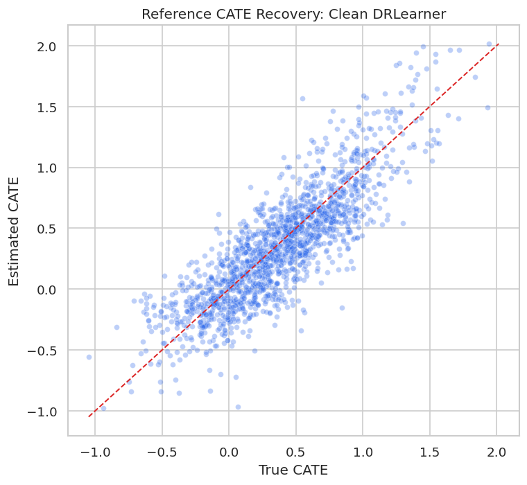

Even the clean reference model has scatter around the diagonal. That is why later reporting should focus on calibrated groups, policy value, and uncertainty rather than claiming exact individual effects.

Pitfall 1: Weak Overlap

Weak overlap means the data contain too few comparable treated and untreated users in parts of the covariate space. In those regions, causal estimates become extrapolation-heavy.

The next cell creates a severe assignment mechanism from the same user features so we can see how overlap problems look.

overlap_demo = data.copy()
# The stress-test assignment function needs complete pre-treatment inputs, so we fill
# only for this diagnostic simulation. This does not change the main modeling matrices.
overlap_assignment_frame = overlap_demo.fillna(overlap_demo.median(numeric_only=True))
overlap_demo["severe_propensity"] = treatment_propensity_function(overlap_assignment_frame, severe=True)
overlap_demo["severe_treatment"] = rng.binomial(1, overlap_demo["severe_propensity"], len(overlap_demo))

overlap_diagnostics = pd.DataFrame(
    {
        "scenario": ["original", "severe_overlap_problem"],
        "min_propensity": [data["true_propensity"].min(), overlap_demo["severe_propensity"].min()],
        "p05_propensity": [data["true_propensity"].quantile(0.05), overlap_demo["severe_propensity"].quantile(0.05)],
        "median_propensity": [data["true_propensity"].median(), overlap_demo["severe_propensity"].median()],
        "p95_propensity": [data["true_propensity"].quantile(0.95), overlap_demo["severe_propensity"].quantile(0.95)],
        "max_propensity": [data["true_propensity"].max(), overlap_demo["severe_propensity"].max()],
        "treatment_rate": [data["treatment"].mean(), overlap_demo["severe_treatment"].mean()],
    }
)
overlap_diagnostics.to_csv(TABLE_DIR / f"{CASE_PREFIX}_overlap_scenario_diagnostics.csv", index=False)
display(overlap_diagnostics)

	scenario	min_propensity	p05_propensity	median_propensity	p95_propensity	max_propensity	treatment_rate
0	original	0.0500	0.1637	0.5119	0.8498	0.9500	0.5148
1	severe_overlap_problem	0.0100	0.0500	0.5232	0.9576	0.9900	0.5198

The severe scenario pushes more users toward near-deterministic treatment assignment. This is the kind of design where an estimator can return numbers, but those numbers may depend heavily on extrapolation.

Propensity Distribution Under Weak Overlap

The plot compares original and severe propensity distributions. Extreme mass near zero or one is the visual signature of overlap failure.

propensity_plot = pd.concat(
    [
        pd.DataFrame({"scenario": "Original", "propensity": data["true_propensity"]}),
        pd.DataFrame({"scenario": "Severe overlap problem", "propensity": overlap_demo["severe_propensity"]}),
    ],
    ignore_index=True,
)

fig, ax = plt.subplots(figsize=(9, 5))
sns.kdeplot(data=propensity_plot, x="propensity", hue="scenario", common_norm=False, fill=True, alpha=0.20, ax=ax)
ax.axvline(0.05, color="#dc2626", linestyle="--", linewidth=1)
ax.axvline(0.95, color="#dc2626", linestyle="--", linewidth=1)
ax.set_title("Propensity Overlap Stress Test")
ax.set_xlabel("Propensity Score")
ax.set_ylabel("Density")
plt.tight_layout()
fig.savefig(FIGURE_DIR / f"{CASE_PREFIX}_overlap_stress_test.png", dpi=160, bbox_inches="tight")
plt.show()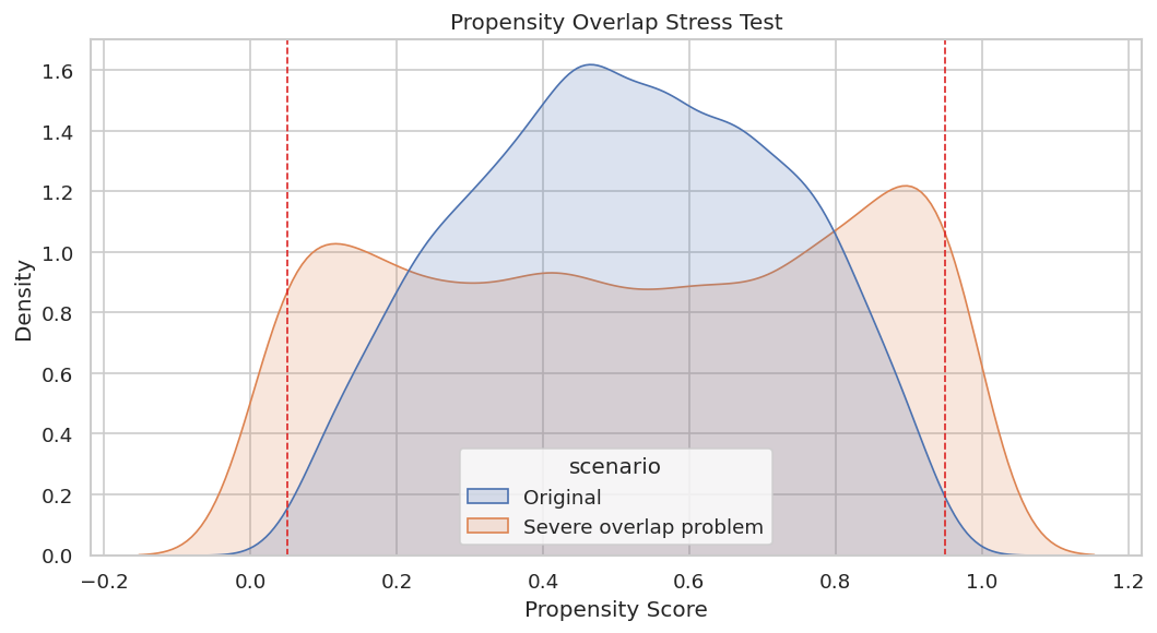

The severe scenario has much more density near the edges. A credible report would either restrict the target population, trim poor-overlap rows, or clearly state that estimates are weak in those regions.

Effective Sample Size Under Weighting

Inverse-propensity weights expose overlap problems numerically. When weights are highly concentrated, the effective sample size becomes much smaller than the raw row count.

def effective_sample_size(weights):
    weights = np.asarray(weights)
    return (weights.sum() ** 2) / np.sum(weights ** 2)

weight_rows = []
for scenario, treatment_col, propensity_col in [
    ("original", "treatment", "true_propensity"),
    ("severe_overlap_problem", "severe_treatment", "severe_propensity"),
]:
    treatment = overlap_demo[treatment_col].to_numpy() if treatment_col in overlap_demo else data[treatment_col].to_numpy()
    propensity = overlap_demo[propensity_col].to_numpy() if propensity_col in overlap_demo else data[propensity_col].to_numpy()
    weights = np.where(treatment == 1, 1 / propensity, 1 / (1 - propensity))
    weight_rows.append(
        {
            "scenario": scenario,
            "rows": len(weights),
            "effective_sample_size": effective_sample_size(weights),
            "max_weight": weights.max(),
            "p99_weight": np.quantile(weights, 0.99),
            "share_weights_above_10": np.mean(weights > 10),
        }
    )
weight_diagnostics = pd.DataFrame(weight_rows)
weight_diagnostics.to_csv(TABLE_DIR / f"{CASE_PREFIX}_weight_effective_sample_size.csv", index=False)
display(weight_diagnostics)

	scenario	rows	effective_sample_size	max_weight	p99_weight	share_weights_above_10
0	original	5200	3,915.0554	20.0000	6.9137	0.0023
1	severe_overlap_problem	5200	1,796.8555	77.9349	13.0630	0.0144

A large raw dataset can behave like a much smaller dataset when overlap is weak. This is a useful reality check before trusting granular CATE estimates.

Pitfall 2: Outcome Leakage

Outcome leakage occurs when a feature contains future outcome information or is built using data unavailable at treatment decision time. The next example adds leaky_outcome_proxy to the effect-modifier set.

This is intentionally wrong. The goal is to show that a model can look strong in a benchmark while being invalid for real deployment.

LEAKY_X_COLUMNS = CLEAN_X_COLUMNS + ["leaky_outcome_proxy"]
X_train_leaky, W_train_leaky, T_train_leaky, Y_train_leaky, X_test_leaky, W_test_leaky, T_test_leaky, Y_test_leaky = build_design(
    train_df,
    test_df,
    LEAKY_X_COLUMNS,
    CLEAN_W_COLUMNS,
)

leaky_estimator = CausalForestDML(
    model_y=make_rf_regressor(301),
    model_t=make_rf_classifier(302),
    discrete_treatment=True,
    n_estimators=128,
    min_samples_leaf=18,
    max_samples=0.45,
    cv=3,
    random_state=RANDOM_STATE + 10,
)
start = time.perf_counter()
leaky_estimator.fit(Y_train_leaky, T_train_leaky, X=X_train_leaky, W=W_train_leaky)
leaky_fit_seconds = time.perf_counter() - start
leaky_effect = leaky_estimator.effect(X_test_leaky)

leaky_metrics = pd.DataFrame(
    [
        summarize_effects("Leaky CausalForestDML", leaky_effect, true_tau_test, leaky_fit_seconds, "Invalid: includes outcome-like future proxy."),
        summarize_effects(best_reference_label, best_reference_effect, true_tau_test, reference_metrics.iloc[0]["fit_seconds"], "Clean reference."),
    ]
).sort_values("cate_rmse")
leaky_metrics.to_csv(TABLE_DIR / f"{CASE_PREFIX}_leakage_metric_comparison.csv", index=False)
display(leaky_metrics)

	analysis	estimated_ate	true_ate_test	ate_bias	cate_rmse	cate_mae	cate_correlation	top_20_true_cate_mean	share_estimated_above_cost	true_net_policy_value	fit_seconds	notes
1	Clean DRLearner	0.3458	0.3723	-0.0266	0.2532	0.1999	0.8484	0.9207	0.6365	0.2813	3.5359	Clean reference.
0	Leaky CausalForestDML	0.0139	0.3723	-0.3584	0.5619	0.4536	0.4902	0.7223	0.0173	0.0190	3.3311	Invalid: includes outcome-like future proxy.

The leaky workflow may look competitive or even attractive by some metrics, but it is invalid because the feature would not be available at decision time. Good metrics cannot rescue a bad feature timeline.

Leakage Timing Check

A simple timing table often catches leakage faster than model diagnostics. Every feature should be available before treatment assignment if it is used for CATE estimation or targeting.

leakage_timing_check = pd.DataFrame(
    {
        "feature": LEAKY_X_COLUMNS + CLEAN_W_COLUMNS,
        "used_in_leaky_model": True,
    }
).merge(field_dictionary[["field", "timing", "modeling_status"]], left_on="feature", right_on="field", how="left")
leakage_timing_check["timing_flag"] = np.where(
    leakage_timing_check["timing"].eq("Pre-treatment"),
    "Allowed timing",
    "Invalid timing for decision-time modeling",
)
leakage_timing_check = leakage_timing_check.drop(columns=["field"])
leakage_timing_check.to_csv(TABLE_DIR / f"{CASE_PREFIX}_leakage_timing_check.csv", index=False)
display(leakage_timing_check.sort_values("timing_flag"))

	feature	used_in_leaky_model	timing	modeling_status	timing_flag
0	need_score	True	Pre-treatment	Allowed X.	Allowed timing
1	prior_activity	True	Pre-treatment	Allowed X.	Allowed timing
2	preference_match	True	Pre-treatment	Allowed X.	Allowed timing
3	search_friction	True	Pre-treatment	Allowed X.	Allowed timing
4	price_sensitivity	True	Pre-treatment	Allowed X.	Allowed timing
5	device_quality	True	Pre-treatment	Allowed X.	Allowed timing
6	high_intent_segment	True	Pre-treatment	Allowed X.	Allowed timing
8	marketing_intensity	True	Pre-treatment	Allowed W.	Allowed timing
9	competitive_pressure	True	Pre-treatment	Allowed W.	Allowed timing
10	market_maturity	True	Pre-treatment	Allowed W.	Allowed timing
11	tenure_weeks	True	Pre-treatment	Allowed W.	Allowed timing
12	organic_source	True	Pre-treatment	Allowed W.	Allowed timing
13	weekday_signup	True	Pre-treatment	Allowed W.	Allowed timing
7	leaky_outcome_proxy	True	Outcome-like leakage	Pitfall: do not use as a feature.	Invalid timing for decision-time modeling

The timing flag is the right conclusion, regardless of the metric table. Leakage is a design error, not a hyperparameter problem.

Pitfall 3: Bad Nuisance Models

DML depends on nuisance models for treatment and outcome. If those nuisance models are too weak, the final treatment-effect estimates can be biased or poorly ranked.

The next cell compares the clean flexible reference with a deliberately simple LinearDML setup.

bad_nuisance_estimator = LinearDML(
    model_y=LinearRegression(),
    model_t=LogisticRegression(max_iter=1_000),
    discrete_treatment=True,
    cv=3,
    random_state=RANDOM_STATE + 20,
)
start = time.perf_counter()
bad_nuisance_estimator.fit(Y_train, T_train, X=X_train, W=W_train)
bad_nuisance_fit_seconds = time.perf_counter() - start
bad_nuisance_effect = bad_nuisance_estimator.effect(X_test)

bad_nuisance_metrics = pd.DataFrame(
    [
        summarize_effects("Too-simple LinearDML", bad_nuisance_effect, true_tau_test, bad_nuisance_fit_seconds, "Uses weak linear nuisance models."),
        summarize_effects(best_reference_label, best_reference_effect, true_tau_test, reference_metrics.iloc[0]["fit_seconds"], "Clean flexible reference."),
    ]
).sort_values("cate_rmse")
bad_nuisance_metrics.to_csv(TABLE_DIR / f"{CASE_PREFIX}_bad_nuisance_comparison.csv", index=False)
display(bad_nuisance_metrics)

	analysis	estimated_ate	true_ate_test	ate_bias	cate_rmse	cate_mae	cate_correlation	top_20_true_cate_mean	share_estimated_above_cost	true_net_policy_value	fit_seconds	notes
0	Too-simple LinearDML	0.3504	0.3723	-0.0219	0.1685	0.1326	0.9280	0.9762	0.6827	0.2914	0.0377	Uses weak linear nuisance models.
1	Clean DRLearner	0.3458	0.3723	-0.0266	0.2532	0.1999	0.8484	0.9207	0.6365	0.2813	3.5359	Clean flexible reference.

The simple nuisance setup is not automatically wrong, but it is risky when the true data-generating process is nonlinear. Nuisance diagnostics help reveal whether that risk is material.

Nuisance Diagnostic Comparison

Here we compare simple and flexible nuisance models directly on the held-out sample. This does not prove the CATE model is correct, but it catches obviously weak adjustment machinery.

XW_train = pd.concat([X_train, W_train], axis=1)
XW_test = pd.concat([X_test, W_test], axis=1)

simple_propensity = LogisticRegression(max_iter=1_000)
simple_propensity.fit(XW_train, T_train)
simple_propensity_pred = np.clip(simple_propensity.predict_proba(XW_test)[:, 1], 1e-4, 1 - 1e-4)

flex_propensity = make_rf_classifier(401)
flex_propensity.fit(XW_train, T_train)
flex_propensity_pred = np.clip(flex_propensity.predict_proba(XW_test)[:, 1], 1e-4, 1 - 1e-4)

simple_outcome = LinearRegression()
simple_outcome.fit(pd.concat([XW_train, T_train.rename("treatment")], axis=1), Y_train)
simple_outcome_pred = simple_outcome.predict(pd.concat([XW_test, T_test.rename("treatment")], axis=1))

flex_outcome = make_rf_regressor(402)
flex_outcome.fit(pd.concat([XW_train, T_train.rename("treatment")], axis=1), Y_train)
flex_outcome_pred = flex_outcome.predict(pd.concat([XW_test, T_test.rename("treatment")], axis=1))

nuisance_comparison = pd.DataFrame(
    [
        {
            "model": "simple_propensity_logistic",
            "task": "treatment",
            "auc": roc_auc_score(T_test, simple_propensity_pred),
            "log_loss": log_loss(T_test, simple_propensity_pred),
            "r2": np.nan,
            "mae": np.nan,
        },
        {
            "model": "flex_propensity_forest",
            "task": "treatment",
            "auc": roc_auc_score(T_test, flex_propensity_pred),
            "log_loss": log_loss(T_test, flex_propensity_pred),
            "r2": np.nan,
            "mae": np.nan,
        },
        {
            "model": "simple_outcome_linear",
            "task": "outcome",
            "auc": np.nan,
            "log_loss": np.nan,
            "r2": r2_score(Y_test, simple_outcome_pred),
            "mae": mean_absolute_error(Y_test, simple_outcome_pred),
        },
        {
            "model": "flex_outcome_forest",
            "task": "outcome",
            "auc": np.nan,
            "log_loss": np.nan,
            "r2": r2_score(Y_test, flex_outcome_pred),
            "mae": mean_absolute_error(Y_test, flex_outcome_pred),
        },
    ]
)
nuisance_comparison.to_csv(TABLE_DIR / f"{CASE_PREFIX}_nuisance_model_comparison.csv", index=False)
display(nuisance_comparison)

	model	task	auc	log_loss	r2	mae
0	simple_propensity_logistic	treatment	0.7623	0.5815	NaN	NaN
1	flex_propensity_forest	treatment	0.7395	0.6020	NaN	NaN
2	simple_outcome_linear	outcome	NaN	NaN	0.5922	0.6025
3	flex_outcome_forest	outcome	NaN	NaN	0.5381	0.6366

When nuisance models perform poorly, treatment-effect estimates deserve extra caution. The CATE model is not separate from the quality of the adjustment stage.

Pitfall 4: Post-Treatment Controls

A post-treatment variable can be a mediator: treatment changes it, and it partly carries the treatment effect to the outcome. If we adjust for it as if it were a confounder, we may estimate a different effect than intended.

The next cell adds post_treatment_activity to W, which is intentionally wrong for the total effect estimand.

POST_CONTROL_W_COLUMNS = CLEAN_W_COLUMNS + ["post_treatment_activity"]
X_train_post, W_train_post, T_train_post, Y_train_post, X_test_post, W_test_post, T_test_post, Y_test_post = build_design(
    train_df,
    test_df,
    CLEAN_X_COLUMNS,
    POST_CONTROL_W_COLUMNS,
)

post_control_estimator = CausalForestDML(
    model_y=make_rf_regressor(501),
    model_t=make_rf_classifier(502),
    discrete_treatment=True,
    n_estimators=128,
    min_samples_leaf=18,
    max_samples=0.45,
    cv=3,
    random_state=RANDOM_STATE + 30,
)
start = time.perf_counter()
post_control_estimator.fit(Y_train_post, T_train_post, X=X_train_post, W=W_train_post)
post_control_fit_seconds = time.perf_counter() - start
post_control_effect = post_control_estimator.effect(X_test_post)

post_control_metrics = pd.DataFrame(
    [
        summarize_effects("Post-treatment control CausalForestDML", post_control_effect, true_tau_test, post_control_fit_seconds, "Invalid for total effect: controls for mediator-like field."),
        summarize_effects(best_reference_label, best_reference_effect, true_tau_test, reference_metrics.iloc[0]["fit_seconds"], "Clean total-effect reference."),
    ]
).sort_values("estimated_ate")
post_control_metrics.to_csv(TABLE_DIR / f"{CASE_PREFIX}_post_treatment_control_comparison.csv", index=False)
display(post_control_metrics)

	analysis	estimated_ate	true_ate_test	ate_bias	cate_rmse	cate_mae	cate_correlation	top_20_true_cate_mean	share_estimated_above_cost	true_net_policy_value	fit_seconds	notes
0	Post-treatment control CausalForestDML	0.3218	0.3723	-0.0505	0.2666	0.2087	0.8733	0.9476	0.7115	0.2805	3.4484	Invalid for total effect: controls for mediato...
1	Clean DRLearner	0.3458	0.3723	-0.0266	0.2532	0.1999	0.8484	0.9207	0.6365	0.2813	3.5359	Clean total-effect reference.

Adding a post-treatment control changes the question being answered. If the target is the total effect of treatment, downstream variables should not be adjusted away as ordinary confounders.

Post-Treatment Field Timing Check

This cell makes the timing violation explicit. A good review process should catch this before the estimator is ever run.

post_control_timing = pd.DataFrame({"feature": CLEAN_X_COLUMNS + POST_CONTROL_W_COLUMNS}).merge(
    field_dictionary[["field", "timing", "modeling_status"]],
    left_on="feature",
    right_on="field",
    how="left",
).drop(columns=["field"])
post_control_timing["timing_flag"] = np.where(
    post_control_timing["timing"].eq("Pre-treatment"),
    "Allowed timing",
    "Invalid for total-effect adjustment",
)
post_control_timing.to_csv(TABLE_DIR / f"{CASE_PREFIX}_post_treatment_timing_check.csv", index=False)
display(post_control_timing.sort_values("timing_flag"))

	feature	timing	modeling_status	timing_flag
0	need_score	Pre-treatment	Allowed X.	Allowed timing
1	prior_activity	Pre-treatment	Allowed X.	Allowed timing
2	preference_match	Pre-treatment	Allowed X.	Allowed timing
3	search_friction	Pre-treatment	Allowed X.	Allowed timing
4	price_sensitivity	Pre-treatment	Allowed X.	Allowed timing
5	device_quality	Pre-treatment	Allowed X.	Allowed timing
6	high_intent_segment	Pre-treatment	Allowed X.	Allowed timing
7	marketing_intensity	Pre-treatment	Allowed W.	Allowed timing
8	competitive_pressure	Pre-treatment	Allowed W.	Allowed timing
9	market_maturity	Pre-treatment	Allowed W.	Allowed timing
10	tenure_weeks	Pre-treatment	Allowed W.	Allowed timing
11	organic_source	Pre-treatment	Allowed W.	Allowed timing
12	weekday_signup	Pre-treatment	Allowed W.	Allowed timing
13	post_treatment_activity	Post-treatment	Pitfall: do not adjust as a confounder.	Invalid for total-effect adjustment

The timing table is more important than whether the post-control model seems accurate. Causal validity is primarily a design issue.

Pitfall 5: Overreading Unit-Level CATE

CATE predictions can rank users reasonably while remaining noisy at the individual level. Decile calibration is a healthier way to discuss heterogeneity than treating every user’s estimate as exact.

calibration_parts = []
comparison_effects = {
    best_reference_label: best_reference_effect,
    "Too-simple LinearDML": bad_nuisance_effect,
    "Leaky CausalForestDML": leaky_effect,
    "Post-treatment control": post_control_effect,
}
for label, estimated in comparison_effects.items():
    temp = pd.DataFrame({"user_id": test_df["user_id"], "true_cate": true_tau_test, "estimated_cate": estimated})
    temp["estimated_decile"] = pd.qcut(temp["estimated_cate"], q=10, labels=False, duplicates="drop") + 1
    summary = (
        temp.groupby("estimated_decile", observed=True)
        .agg(users=("user_id", "size"), mean_estimated_cate=("estimated_cate", "mean"), mean_true_cate=("true_cate", "mean"))
        .reset_index()
    )
    summary["analysis"] = label
    calibration_parts.append(summary)

calibration_table = pd.concat(calibration_parts, ignore_index=True)
calibration_table.to_csv(TABLE_DIR / f"{CASE_PREFIX}_decile_calibration_comparison.csv", index=False)
display(calibration_table.head(15))

	estimated_decile	users	mean_estimated_cate	mean_true_cate	analysis
0	1	156	-0.3712	-0.2142	Clean DRLearner
1	2	156	-0.1326	-0.0505	Clean DRLearner
2	3	156	0.0006	0.0596	Clean DRLearner
3	4	156	0.1402	0.1905	Clean DRLearner
4	5	156	0.2685	0.3146	Clean DRLearner
5	6	156	0.3848	0.4333	Clean DRLearner
6	7	156	0.4985	0.5173	Clean DRLearner
7	8	156	0.6140	0.6313	Clean DRLearner
8	9	156	0.7944	0.7605	Clean DRLearner
9	10	156	1.2603	1.0810	Clean DRLearner
10	1	156	-0.3700	-0.3116	Too-simple LinearDML
11	2	156	-0.0826	-0.0671	Too-simple LinearDML
12	3	156	0.0648	0.0804	Too-simple LinearDML
13	4	156	0.1937	0.1900	Too-simple LinearDML
14	5	156	0.3024	0.3075	Too-simple LinearDML

A useful CATE model should show higher true effects in higher estimated deciles. If that pattern is weak or inconsistent, the model should not drive precise individual-level claims.

Decile Calibration Plot

The plot shows whether estimated deciles correspond to real effect differences. This is a better communication device than a long list of user-level predictions.

calibration_plot = calibration_table.melt(
    id_vars=["analysis", "estimated_decile", "users"],
    value_vars=["mean_estimated_cate", "mean_true_cate"],
    var_name="series",
    value_name="cate",
)
calibration_plot["series"] = calibration_plot["series"].map({"mean_estimated_cate": "Estimated", "mean_true_cate": "True"})

g = sns.relplot(
    data=calibration_plot,
    x="estimated_decile",
    y="cate",
    hue="series",
    col="analysis",
    col_wrap=2,
    kind="line",
    marker="o",
    height=3.5,
    facet_kws={"sharey": True},
)
g.set_axis_labels("Estimated CATE Decile", "Average CATE")
g.fig.suptitle("Decile Calibration Across Clean And Problematic Workflows", y=1.02)
plt.tight_layout()
g.fig.savefig(FIGURE_DIR / f"{CASE_PREFIX}_decile_calibration_comparison.png", dpi=160, bbox_inches="tight")
plt.show()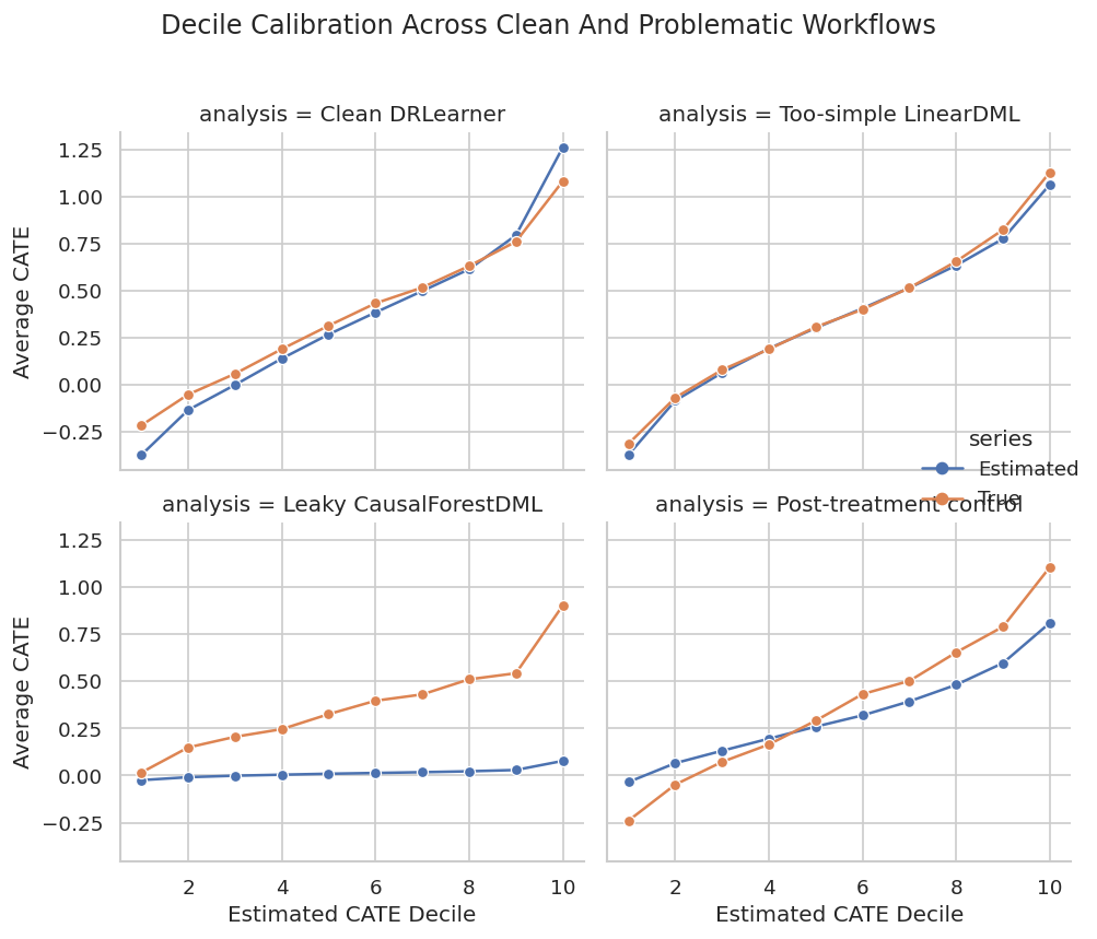

Calibration plots make overclaiming harder. A model may still be useful for coarse targeting even when individual-level predictions are noisy.

Pitfall 6: Segment Hunting

If analysts search enough segments, some will appear unusually high or low by chance. The next cell creates random segments unrelated to the causal design and measures how extreme their apparent true effects can look.

segment_rng = np.random.default_rng(RANDOM_STATE + 77)
random_segment_rows = []
for segment_id in range(1, 81):
    segment_share = segment_rng.uniform(0.08, 0.35)
    segment_mask = segment_rng.random(len(test_df)) < segment_share
    if segment_mask.sum() < 30:
        continue
    random_segment_rows.append(
        {
            "segment": f"random_segment_{segment_id:02d}",
            "users": int(segment_mask.sum()),
            "mean_true_cate": true_tau_test[segment_mask].mean(),
            "mean_reference_cate": best_reference_effect[segment_mask].mean(),
            "reference_minus_true": best_reference_effect[segment_mask].mean() - true_tau_test[segment_mask].mean(),
        }
    )
random_segment_scan = pd.DataFrame(random_segment_rows).sort_values("mean_reference_cate", ascending=False)
random_segment_scan.to_csv(TABLE_DIR / f"{CASE_PREFIX}_random_segment_scan.csv", index=False)
display(random_segment_scan.head(10))

	segment	users	mean_true_cate	mean_reference_cate	reference_minus_true
36	random_segment_37	123	0.4217	0.4118	-0.0099
4	random_segment_05	119	0.4246	0.4007	-0.0239
52	random_segment_53	252	0.4292	0.4000	-0.0292
33	random_segment_34	178	0.4011	0.3921	-0.0090
59	random_segment_60	527	0.4138	0.3881	-0.0258
72	random_segment_73	325	0.4011	0.3815	-0.0196
37	random_segment_38	467	0.3948	0.3799	-0.0149
19	random_segment_20	322	0.4001	0.3794	-0.0207
0	random_segment_01	259	0.3844	0.3778	-0.0066
57	random_segment_58	309	0.3835	0.3732	-0.0104

Some random segments can look impressive simply because many were searched. Segment results should be pre-specified when possible, and exploratory segments should be labeled as exploratory.

Random Segment Distribution

The distribution of random segment means shows how much apparent heterogeneity can appear even when the segments are arbitrary.

fig, ax = plt.subplots(figsize=(9, 5))
sns.histplot(random_segment_scan["mean_reference_cate"], bins=25, color="#7c3aed", alpha=0.75, ax=ax)
ax.axvline(best_reference_effect.mean(), color="#111827", linewidth=1.4, label="Overall estimated ATE")
ax.set_title("Exploratory Random Segment Estimates")
ax.set_xlabel("Mean Estimated CATE In Random Segment")
ax.set_ylabel("Segments")
ax.legend()
plt.tight_layout()
fig.savefig(FIGURE_DIR / f"{CASE_PREFIX}_random_segment_hunting.png", dpi=160, bbox_inches="tight")
plt.show()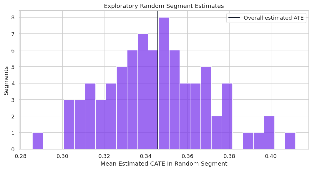

This plot is a warning against cherry-picked segment stories. A credible report should distinguish planned segments from exploratory discoveries.

Policy Value Comparison Across Workflows

The next table translates each workflow into a simple rule: treat users with estimated CATE above cost. This reveals how design mistakes affect decisions, not just model metrics.

policy_rows = []
for label, estimated in comparison_effects.items():
    action = estimated > TREATMENT_COST
    policy_rows.append(
        {
            "analysis": label,
            "treatment_rate": action.mean(),
            "users_treated": int(action.sum()),
            "mean_true_cate_among_treated": true_tau_test[action].mean() if action.sum() else np.nan,
            "precision_positive_net": np.mean(true_tau_test[action] > TREATMENT_COST) if action.sum() else np.nan,
            "true_net_value_per_user": ((true_tau_test - TREATMENT_COST) * action).mean(),
        }
    )
policy_rows.extend(
    [
        {
            "analysis": "Treat none",
            "treatment_rate": 0.0,
            "users_treated": 0,
            "mean_true_cate_among_treated": np.nan,
            "precision_positive_net": np.nan,
            "true_net_value_per_user": 0.0,
        },
        {
            "analysis": "Treat all",
            "treatment_rate": 1.0,
            "users_treated": len(test_df),
            "mean_true_cate_among_treated": true_tau_test.mean(),
            "precision_positive_net": np.mean(true_tau_test > TREATMENT_COST),
            "true_net_value_per_user": (true_tau_test - TREATMENT_COST).mean(),
        },
    ]
)
policy_comparison = pd.DataFrame(policy_rows).sort_values("true_net_value_per_user", ascending=False)
policy_comparison.to_csv(TABLE_DIR / f"{CASE_PREFIX}_policy_value_comparison.csv", index=False)
display(policy_comparison)

	analysis	treatment_rate	users_treated	mean_true_cate_among_treated	precision_positive_net	true_net_value_per_user
1	Too-simple LinearDML	0.6827	1065	0.5868	0.9070	0.2914
0	Clean DRLearner	0.6365	993	0.6018	0.9033	0.2813
3	Post-treatment control	0.7115	1110	0.5542	0.8613	0.2805
5	Treat all	1.0000	1560	0.3723	0.6679	0.2123
2	Leaky CausalForestDML	0.0173	27	1.2598	1.0000	0.0190
4	Treat none	0.0000	0	NaN	NaN	0.0000

Policy value is the practical consequence of modeling choices. Invalid designs should still be rejected even if their policy table looks good in this simulated benchmark.

Policy Value Plot

This plot compares net value per held-out user across clean and problematic workflows. The invalid analyses are included to show why the diagnostics matter.

fig, ax = plt.subplots(figsize=(10, 5.5))
plot_policy = policy_comparison.sort_values("true_net_value_per_user")
sns.barplot(data=plot_policy, x="true_net_value_per_user", y="analysis", color="#22c55e", ax=ax)
ax.axvline(0, color="#111827", linewidth=1)
ax.set_title("Policy Value Across Clean And Problematic Workflows")
ax.set_xlabel("True Net Value Per User")
ax.set_ylabel("")
plt.tight_layout()
fig.savefig(FIGURE_DIR / f"{CASE_PREFIX}_policy_value_comparison.png", dpi=160, bbox_inches="tight")
plt.show()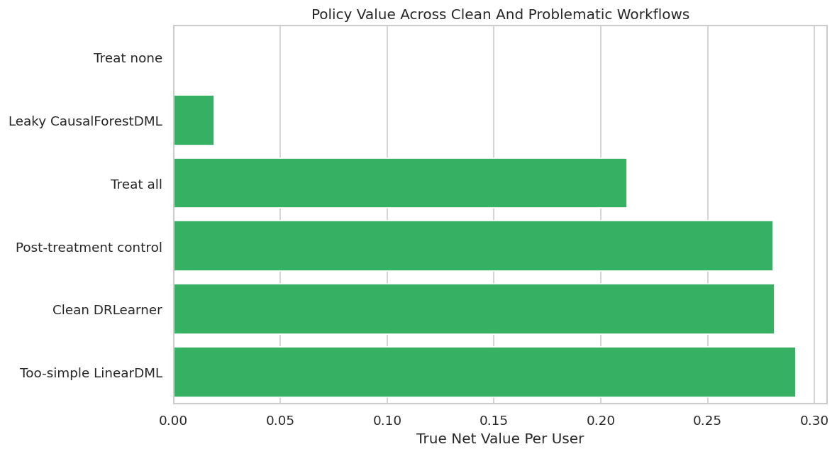

The chart is useful only when read together with validity checks. A design can generate value in a teaching simulation and still be unusable in real deployment because it relies on future information or changes the estimand.

Bootstrap Policy Uncertainty

A single held-out value can be noisy. Bootstrapping held-out rows shows how much policy value changes across plausible evaluation samples.

bootstrap_rng = np.random.default_rng(RANDOM_STATE + 123)
N_BOOTSTRAPS = 300
policy_actions = {label: (estimated > TREATMENT_COST) for label, estimated in comparison_effects.items()}
policy_actions["Treat none"] = np.zeros(len(test_df), dtype=bool)
policy_actions["Treat all"] = np.ones(len(test_df), dtype=bool)

bootstrap_rows = []
for draw in range(N_BOOTSTRAPS):
    sample_index = bootstrap_rng.choice(len(test_df), size=len(test_df), replace=True)
    for label, action in policy_actions.items():
        value = ((true_tau_test[sample_index] - TREATMENT_COST) * action[sample_index]).mean()
        bootstrap_rows.append({"draw": draw, "analysis": label, "true_net_value_per_user": value})
bootstrap_policy = pd.DataFrame(bootstrap_rows)
bootstrap_policy_summary = (
    bootstrap_policy.groupby("analysis")
    .agg(
        mean_value=("true_net_value_per_user", "mean"),
        lower_95=("true_net_value_per_user", lambda values: np.quantile(values, 0.025)),
        upper_95=("true_net_value_per_user", lambda values: np.quantile(values, 0.975)),
    )
    .reset_index()
    .sort_values("mean_value", ascending=False)
)
bootstrap_policy.to_csv(TABLE_DIR / f"{CASE_PREFIX}_bootstrap_policy_values.csv", index=False)
bootstrap_policy_summary.to_csv(TABLE_DIR / f"{CASE_PREFIX}_bootstrap_policy_summary.csv", index=False)
display(bootstrap_policy_summary)

	analysis	mean_value	lower_95	upper_95
3	Too-simple LinearDML	0.2916	0.2747	0.3080
0	Clean DRLearner	0.2816	0.2653	0.2972
2	Post-treatment control	0.2807	0.2641	0.2977
4	Treat all	0.2126	0.1903	0.2342
1	Leaky CausalForestDML	0.0193	0.0122	0.0266
5	Treat none	0.0000	0.0000	0.0000

Bootstrap intervals help avoid false precision. If two valid policies overlap heavily, the report should not oversell their ordering.

Bootstrap Policy Interval Plot

The interval plot summarizes the uncertainty around each policy’s net value. Invalid workflows remain labeled as workflows, but they should not be recommended.

plot_bootstrap = bootstrap_policy_summary.sort_values("mean_value")
fig, ax = plt.subplots(figsize=(10, 6))
ax.errorbar(
    x=plot_bootstrap["mean_value"],
    y=plot_bootstrap["analysis"],
    xerr=[
        plot_bootstrap["mean_value"] - plot_bootstrap["lower_95"],
        plot_bootstrap["upper_95"] - plot_bootstrap["mean_value"],
    ],
    fmt="o",
    color="#2563eb",
    ecolor="#334155",
    capsize=4,
)
ax.axvline(0, color="#111827", linewidth=1)
ax.set_title("Bootstrap Uncertainty Around Policy Value")
ax.set_xlabel("True Net Value Per User")
ax.set_ylabel("")
plt.tight_layout()
fig.savefig(FIGURE_DIR / f"{CASE_PREFIX}_bootstrap_policy_intervals.png", dpi=160, bbox_inches="tight")
plt.show()

The interval view encourages a more measured conclusion. It also makes clear why model comparison should include uncertainty, not just rank ordering.

Consolidated Failure Mode Scorecard

This scorecard collects the major examples in one place. The key column is not the metric value alone; it is whether the workflow is valid for the intended total-effect decision.

all_metric_rows = pd.concat(
    [
        reference_metrics,
        leaky_metrics[leaky_metrics["analysis"].eq("Leaky CausalForestDML")],
        bad_nuisance_metrics[bad_nuisance_metrics["analysis"].eq("Too-simple LinearDML")],
        post_control_metrics[post_control_metrics["analysis"].eq("Post-treatment control CausalForestDML")],
    ],
    ignore_index=True,
)
validity_map = {
    "Clean CausalForestDML": "Valid design, subject to unconfoundedness and overlap.",
    "Clean DRLearner": "Valid design, subject to unconfoundedness and overlap.",
    "Leaky CausalForestDML": "Invalid: uses outcome-like future information.",
    "Too-simple LinearDML": "Valid timing, but high model-risk if nuisance models are misspecified.",
    "Post-treatment control CausalForestDML": "Invalid for total effect: adjusts for downstream variable.",
}
scorecard = all_metric_rows[[
    "analysis",
    "estimated_ate",
    "ate_bias",
    "cate_rmse",
    "cate_correlation",
    "true_net_policy_value",
    "fit_seconds",
]].copy()
scorecard["validity_assessment"] = scorecard["analysis"].map(validity_map)
scorecard = scorecard.sort_values("true_net_policy_value", ascending=False)
scorecard.to_csv(TABLE_DIR / f"{CASE_PREFIX}_failure_mode_scorecard.csv", index=False)
display(scorecard)

	analysis	estimated_ate	ate_bias	cate_rmse	cate_correlation	true_net_policy_value	fit_seconds	validity_assessment
3	Too-simple LinearDML	0.3504	-0.0219	0.1685	0.9280	0.2914	0.0377	Valid timing, but high model-risk if nuisance ...
1	Clean CausalForestDML	0.3609	-0.0115	0.2667	0.8733	0.2815	3.6758	Valid design, subject to unconfoundedness and ...
0	Clean DRLearner	0.3458	-0.0266	0.2532	0.8484	0.2813	3.5359	Valid design, subject to unconfoundedness and ...
4	Post-treatment control CausalForestDML	0.3218	-0.0505	0.2666	0.8733	0.2805	3.4484	Invalid for total effect: adjusts for downstre...
2	Leaky CausalForestDML	0.0139	-0.3584	0.5619	0.4902	0.0190	3.3311	Invalid: uses outcome-like future information.

The scorecard demonstrates a central reporting habit: separate performance from validity. Invalid workflows should not become recommendations just because they score well.

Debugging Playbook

The playbook turns the notebook examples into a sequence of questions to ask whenever an EconML result looks surprising.

debugging_playbook = pd.DataFrame(
    [
        ("Effect estimate is much larger than expected", "Check leakage, post-treatment controls, target population mismatch, and raw treated-control imbalance."),
        ("CATE estimates look extremely spread out", "Check overlap, nuisance model instability, small leaves, and whether X includes noisy identifiers."),
        ("Policy treats almost everyone", "Compare estimated CATE distribution to cost and inspect propensity support among treated recommendations."),
        ("Top segment looks too good", "Confirm the segment was pre-specified and compare against random segment scans."),
        ("Estimator rankings disagree", "Compare nuisance diagnostics, calibration, segment behavior, and bootstrap intervals rather than choosing by one metric."),
        ("Confidence seems too high", "Check sample size, overlap, repeated model selection, and whether uncertainty includes policy-selection uncertainty."),
        ("A feature is very predictive", "Audit whether it exists before treatment and whether it is a mediator, collider, or outcome proxy."),
    ],
    columns=["symptom", "first_debugging_moves"],
)
debugging_playbook.to_csv(TABLE_DIR / f"{CASE_PREFIX}_debugging_playbook.csv", index=False)
display(debugging_playbook)

	symptom	first_debugging_moves
0	Effect estimate is much larger than expected	Check leakage, post-treatment controls, target...
1	CATE estimates look extremely spread out	Check overlap, nuisance model instability, sma...
2	Policy treats almost everyone	Compare estimated CATE distribution to cost an...
3	Top segment looks too good	Confirm the segment was pre-specified and comp...
4	Estimator rankings disagree	Compare nuisance diagnostics, calibration, seg...
5	Confidence seems too high	Check sample size, overlap, repeated model sel...
6	A feature is very predictive	Audit whether it exists before treatment and w...

The playbook is intentionally practical. Most debugging starts with a suspicious result and then works backward through timing, overlap, model quality, and decision logic.

Reporting Checklist

A transparent causal report should make assumptions and diagnostics visible. The checklist below is designed for EconML analyses, but the same structure works for most observational causal projects.

reporting_checklist = pd.DataFrame(
    [
        ("Causal question", "Treatment, outcome, target population, and estimand are written plainly."),
        ("Feature timing", "Every model feature is confirmed to be pre-treatment for the target decision."),
        ("Confounder logic", "The report explains why included controls are plausible confounders and what may be missing."),
        ("Overlap", "Propensity distributions, bucket counts, or support filters are shown."),
        ("Nuisance models", "Treatment and outcome nuisance diagnostics are reported."),
        ("Estimator comparison", "Results are checked across at least one reasonable alternative estimator or specification."),
        ("Heterogeneity", "CATE claims are summarized by calibrated groups or segments, not only individual scores."),
        ("Policy value", "Treatment cost, threshold rule, treatment rate, and net value are reported."),
        ("Uncertainty", "Intervals or bootstrap checks are included for key estimates or policy values."),
        ("Limitations", "Unobserved confounding, overlap gaps, measurement limits, and validation needs are stated."),
    ],
    columns=["report_section", "what_to_include"],
)
reporting_checklist.to_csv(TABLE_DIR / f"{CASE_PREFIX}_reporting_checklist.csv", index=False)
display(reporting_checklist)

	report_section	what_to_include
0	Causal question	Treatment, outcome, target population, and est...
1	Feature timing	Every model feature is confirmed to be pre-tre...
2	Confounder logic	The report explains why included controls are ...
3	Overlap	Propensity distributions, bucket counts, or su...
4	Nuisance models	Treatment and outcome nuisance diagnostics are...
5	Estimator comparison	Results are checked across at least one reason...
6	Heterogeneity	CATE claims are summarized by calibrated group...
7	Policy value	Treatment cost, threshold rule, treatment rate...
8	Uncertainty	Intervals or bootstrap checks are included for...
9	Limitations	Unobserved confounding, overlap gaps, measurem...

The checklist makes the final result reviewable. A model output without these ingredients should be treated as a preliminary analysis, not a decision-ready causal estimate.

Short Report Template

The final code cell writes a compact markdown report template using the notebook’s computed results. It emphasizes validity, not only performance.

best_valid_policy = policy_comparison[policy_comparison["analysis"].isin(list(reference_effects.keys()))].iloc[0]
best_valid_metric = reference_metrics.iloc[0]

report_lines = [
    "# EconML Debugging And Reporting Summary",
    "",
    "## Recommended Valid Workflow",
    "",
    f"The strongest valid reference workflow in this teaching run is **{best_valid_metric['analysis']}**.",
    "",
    f"- Held-out CATE RMSE: `{best_valid_metric['cate_rmse']:.4f}`",
    f"- Held-out CATE correlation: `{best_valid_metric['cate_correlation']:.4f}`",
    f"- Net policy value per user: `{best_valid_policy['true_net_value_per_user']:.4f}`",
    f"- Treatment rate under cost threshold: `{best_valid_policy['treatment_rate']:.1%}`",
    "",
    "## Main Lessons",
    "",
    "1. Strong-looking metrics do not fix invalid feature timing.",
    "2. Weak overlap reduces the effective information available for causal estimation.",
    "3. Bad nuisance models can distort both average and heterogeneous effects.",
    "4. Post-treatment controls can change the estimand by blocking part of the treatment pathway.",
    "5. CATE estimates should be reported with calibration, segment checks, policy value, and uncertainty.",
    "",
    "## Required Caveats",
    "",
    "This notebook uses synthetic data with known truth. In real observational analysis, the report must include domain justification for confounders, evidence of overlap, sensitivity to modeling choices, and validation plans before a policy recommendation is treated as decision-ready.",
]
report_text = "\n".join(report_lines)
report_path = REPORT_DIR / f"{CASE_PREFIX}_debugging_reporting_summary.md"
report_path.write_text(report_text)
display(Markdown(report_text))
print(f"Saved report to: {report_path}")

EconML Debugging And Reporting Summary

Recommended Valid Workflow

The strongest valid reference workflow in this teaching run is Clean DRLearner.

Held-out CATE RMSE: 0.2532
Held-out CATE correlation: 0.8484
Net policy value per user: 0.2813
Treatment rate under cost threshold: 63.7%

Main Lessons

Strong-looking metrics do not fix invalid feature timing.
Weak overlap reduces the effective information available for causal estimation.
Bad nuisance models can distort both average and heterogeneous effects.
Post-treatment controls can change the estimand by blocking part of the treatment pathway.
CATE estimates should be reported with calibration, segment checks, policy value, and uncertainty.

Required Caveats

This notebook uses synthetic data with known truth. In real observational analysis, the report must include domain justification for confounders, evidence of overlap, sensitivity to modeling choices, and validation plans before a policy recommendation is treated as decision-ready.

Saved report to: /home/apex/Documents/ranking_sys/notebooks/tutorials/econml/outputs/reports/15_debugging_reporting_summary.md

The report template closes the tutorial series on the right note: the best causal analysis is not the one with the fanciest estimator, but the one whose design, diagnostics, limitations, and decision logic are clear.

Final Takeaways

EconML is powerful when the causal question is well-defined and the analyst respects the assumptions. The recurring pattern across this tutorial sequence is simple: define the estimand, protect feature timing, diagnose overlap, check nuisance models, validate heterogeneity at group level, quantify policy value, and report limitations honestly.

That discipline is what turns treatment-effect modeling from an impressive notebook into credible applied causal work.