EconML Tutorial 10: Multiple Treatments And Continuous Treatments

Most introductory causal examples use a binary treatment: treated or not treated. Real decision systems are often richer than that. A product team might choose among several intervention types, a pricing team might choose a discount amount, and an operations team might choose how much support or attention to allocate.

This notebook extends the EconML tutorial sequence beyond binary treatment in two directions:

• multiple discrete treatments, where the decision is one of several mutually exclusive arms;
• continuous treatments, where the decision is a dose, intensity, price, time, or quantity.

These settings require a careful shift in language. Instead of asking only “what is the effect of treatment versus control?”, we ask:

• What is the effect of arm 1 versus control?
• What is the effect of arm 2 versus control?
• Which arm has the largest expected gain for a given covariate profile?
• How much does the outcome change when the continuous treatment increases by one unit?
• Does the estimated marginal effect vary across segments?

We will use synthetic teaching data with known ground truth, so we can check whether the estimators recover the right arm rankings and dose-response slopes.

Learning Goals

By the end of this notebook, you should be able to:

• define estimands for multi-arm and continuous-treatment settings;
• simulate confounded multi-arm treatment assignment and continuous treatment intensity;
• use DRLearner for multi-arm heterogeneous treatment effects;
• estimate treatment effects for each arm relative to a control arm;
• translate arm-specific CATE estimates into an estimated best-arm policy;
• use LinearDML for continuous treatment effects;
• interpret marginal effects and finite dose contrasts;
• diagnose overlap, dose support, and segment-level treatment-effect recovery.

Tutorial Flow

The notebook has two teaching case studies.

First, we build a three-arm discrete treatment dataset. We fit an EconML DRLearner, estimate effects for each active arm versus control, and evaluate an estimated best-arm policy against the known synthetic truth.

Second, we build a continuous-dose dataset. We fit LinearDML, estimate heterogeneous marginal dose effects, compare them with the true slope, and inspect where the estimated dose effect is strongest.

The two parts use different estimators because the treatment structure is different. That is the main lesson: the causal question determines the estimator interface.

Setup

This cell imports the notebook dependencies, creates output folders, and sets plotting defaults. The warning filters remove harmless display and pandas-to-NumPy conversion messages so the saved notebook stays readable.

from pathlib import Path
import os
import warnings

# Suppress optional widget warnings that can appear while importing EconML in headless notebook runs.
warnings.filterwarnings("ignore", message="IProgress not found.*")

# Keep Matplotlib cache files in a writable location during notebook execution.
os.environ.setdefault("MPLCONFIGDIR", "/tmp/matplotlib")

import econml
import matplotlib.pyplot as plt
from matplotlib.ticker import PercentFormatter
import numpy as np
import pandas as pd
import seaborn as sns
from IPython.display import display
from scipy.special import softmax
from sklearn.ensemble import RandomForestClassifier, RandomForestRegressor
from sklearn.linear_model import LogisticRegression
from sklearn.metrics import accuracy_score, log_loss, mean_absolute_error, mean_squared_error, roc_auc_score
from sklearn.model_selection import train_test_split

from econml.dr import DRLearner
from econml.dml import LinearDML

warnings.filterwarnings("ignore", message="X does not have valid feature names.*", category=UserWarning)
warnings.filterwarnings("ignore", message="Not all column names are strings.*", category=UserWarning)
warnings.filterwarnings("ignore", category=FutureWarning)

sns.set_theme(style="whitegrid", context="notebook")
plt.rcParams["figure.figsize"] = (10, 6)
plt.rcParams["axes.titleweight"] = "bold"
plt.rcParams["axes.labelsize"] = 11


def find_project_root(start=None):
    """Find the repository root from either the repo or a nested notebook folder."""
    start = Path.cwd() if start is None else Path(start)
    for candidate in [start, *start.parents]:
        if (candidate / "pyproject.toml").exists() and (candidate / "notebooks").exists():
            return candidate
    return Path.cwd()


PROJECT_ROOT = find_project_root()
NOTEBOOK_DIR = PROJECT_ROOT / "notebooks" / "tutorials" / "econml"
OUTPUT_DIR = NOTEBOOK_DIR / "outputs"
FIGURE_DIR = OUTPUT_DIR / "figures"
TABLE_DIR = OUTPUT_DIR / "tables"

FIGURE_DIR.mkdir(parents=True, exist_ok=True)
TABLE_DIR.mkdir(parents=True, exist_ok=True)

rng = np.random.default_rng(202610)

print(f"Project root: {PROJECT_ROOT}")
print(f"EconML version: {econml.__version__}")
print(f"Figures will be saved to: {FIGURE_DIR.relative_to(PROJECT_ROOT)}")
print(f"Tables will be saved to: {TABLE_DIR.relative_to(PROJECT_ROOT)}")

Project root: /home/apex/Documents/ranking_sys
EconML version: 0.16.0
Figures will be saved to: notebooks/tutorials/econml/outputs/figures
Tables will be saved to: notebooks/tutorials/econml/outputs/tables

The environment is ready. We will save all tables and plots with the 10_ prefix so they remain easy to separate from earlier tutorial outputs.

Estimand Map

Multi-arm and continuous-treatment problems use different estimands. This table gives the vocabulary we will use before the code starts creating data.

estimand_map = pd.DataFrame(
    [
        {
            "setting": "Binary treatment",
            "treatment_example": "0 or 1",
            "estimand": "Effect of treatment 1 versus treatment 0",
            "econml_call_pattern": "est.effect(X)",
            "decision_question": "Should this unit receive the intervention?",
        },
        {
            "setting": "Multiple discrete treatments",
            "treatment_example": "0, 1, or 2",
            "estimand": "Effect of each active arm versus a baseline arm",
            "econml_call_pattern": "est.effect(X, T0=0, T1=arm)",
            "decision_question": "Which arm should this unit receive?",
        },
        {
            "setting": "Continuous treatment",
            "treatment_example": "Dose, intensity, discount, exposure time",
            "estimand": "Marginal effect of increasing the treatment by one unit",
            "econml_call_pattern": "est.const_marginal_effect(X) or est.effect(X, T0=a, T1=b)",
            "decision_question": "How much should the treatment intensity change?",
        },
    ]
)

estimand_map.to_csv(TABLE_DIR / "10_estimand_map.csv", index=False)
display(estimand_map)

	setting	treatment_example	estimand	econml_call_pattern	decision_question
0	Binary treatment	0 or 1	Effect of treatment 1 versus treatment 0	est.effect(X)	Should this unit receive the intervention?
1	Multiple discrete treatments	0, 1, or 2	Effect of each active arm versus a baseline arm	est.effect(X, T0=0, T1=arm)	Which arm should this unit receive?
2	Continuous treatment	Dose, intensity, discount, exposure time	Marginal effect of increasing the treatment by...	est.const_marginal_effect(X) or est.effect(X, ...	How much should the treatment intensity change?

The key distinction is the contrast. Multi-arm treatment effects are relative to another arm, while continuous-treatment effects are usually marginal slopes or finite dose changes.

Part A: Multiple Discrete Treatments

In this section, the treatment has three possible arms. Arm 0 is the baseline experience. Arm 1 is a guided personalization intervention. Arm 2 is an exploration-oriented intervention. Each active arm helps different kinds of rows.

Multi-Arm Treatment Definitions

A multi-arm analysis should name each treatment arm clearly before modeling. This avoids a common mistake: interpreting arm-specific CATE estimates without remembering which baseline they are relative to.

arm_dictionary = pd.DataFrame(
    [
        {
            "arm": 0,
            "name": "baseline experience",
            "description": "No active intervention beyond the standard experience.",
            "role": "Reference arm for treatment-effect contrasts.",
        },
        {
            "arm": 1,
            "name": "guided personalization",
            "description": "A focused intervention intended to help high-need, already-engaged rows.",
            "role": "Active arm compared against baseline.",
        },
        {
            "arm": 2,
            "name": "exploration boost",
            "description": "A broader discovery-oriented intervention intended to help novelty-seeking rows.",
            "role": "Active arm compared against baseline.",
        },
    ]
)

arm_dictionary.to_csv(TABLE_DIR / "10_multi_arm_dictionary.csv", index=False)
display(arm_dictionary)

	arm	name	description	role
0	0	baseline experience	No active intervention beyond the standard exp...	Reference arm for treatment-effect contrasts.
1	1	guided personalization	A focused intervention intended to help high-n...	Active arm compared against baseline.
2	2	exploration boost	A broader discovery-oriented intervention inte...	Active arm compared against baseline.

The reference arm is arm 0. Every arm-specific effect we estimate in this section will be read as “switching from baseline to this arm,” unless explicitly stated otherwise.

Multi-Arm Teaching Data

This cell creates a confounded three-arm observational dataset. Treatment assignment depends on observed covariates, and each active arm has its own heterogeneous treatment effect. Because we know the true arm effects, we can evaluate whether the model learns the right contrasts.

def true_arm_effects(frame):
    """Return true treatment effects for arm 1 and arm 2 versus baseline."""
    tau_arm_1 = (
        0.25
        + 0.34 * frame["baseline_need"]
        + 0.18 * frame["prior_engagement"]
        - 0.22 * np.maximum(frame["friction_score"], 0)
        + 0.16 * frame["content_affinity"]
        - 0.12 * frame["price_sensitivity"]
        + 0.14 * frame["high_need_segment"] * (frame["content_affinity"] > 0).astype(float)
    )
    tau_arm_2 = (
        0.18
        + 0.42 * frame["novelty_preference"]
        + 0.18 * frame["content_affinity"]
        - 0.18 * frame["friction_score"]
        - 0.22 * frame["price_sensitivity"]
        + 0.20 * frame["low_friction_segment"]
        - 0.16 * frame["region_risk"]
    )
    return tau_arm_1, tau_arm_2


n_multi = 4_200
baseline_need = rng.normal(0, 1, size=n_multi)
prior_engagement = rng.normal(0, 1, size=n_multi)
friction_score = rng.normal(0, 1, size=n_multi)
content_affinity = rng.normal(0, 1, size=n_multi)
novelty_preference = rng.normal(0, 1, size=n_multi)
price_sensitivity = rng.beta(2.0, 3.2, size=n_multi)
account_tenure = rng.gamma(shape=3.2, scale=16.0, size=n_multi)
region_risk = rng.binomial(1, 0.30, size=n_multi)
high_need_segment = (baseline_need > 0.55).astype(int)
low_friction_segment = (friction_score < -0.25).astype(int)

multi_features = pd.DataFrame(
    {
        "baseline_need": baseline_need,
        "prior_engagement": prior_engagement,
        "friction_score": friction_score,
        "content_affinity": content_affinity,
        "novelty_preference": novelty_preference,
        "price_sensitivity": price_sensitivity,
        "account_tenure": account_tenure,
        "region_risk": region_risk,
        "high_need_segment": high_need_segment,
        "low_friction_segment": low_friction_segment,
    }
)

tau_arm_1, tau_arm_2 = true_arm_effects(multi_features)

# Softmax assignment creates three probabilities that sum to one for every row.
assignment_logits = np.column_stack(
    [
        np.zeros(n_multi),
        -0.15 + 0.55 * baseline_need + 0.35 * prior_engagement - 0.25 * friction_score + 0.15 * high_need_segment,
        -0.25 + 0.60 * novelty_preference + 0.28 * content_affinity - 0.35 * friction_score - 0.20 * price_sensitivity,
    ]
)
arm_probabilities = softmax(assignment_logits, axis=1)
treatment_arm = np.array([rng.choice([0, 1, 2], p=row) for row in arm_probabilities])

base_outcome = (
    1.20
    + 0.52 * baseline_need
    + 0.42 * prior_engagement
    - 0.30 * friction_score
    + 0.28 * content_affinity
    + 0.18 * novelty_preference
    - 0.20 * price_sensitivity
    + 0.10 * np.log1p(account_tenure)
    - 0.18 * region_risk
)
observed_arm_effect = np.select([treatment_arm == 1, treatment_arm == 2], [tau_arm_1, tau_arm_2], default=0.0)
noise = rng.normal(0, 0.72 + 0.12 * np.maximum(friction_score, 0), size=n_multi)
outcome = base_outcome + observed_arm_effect + noise

multi_df = multi_features.assign(
    treatment_arm=treatment_arm,
    outcome=outcome,
    true_tau_arm_1=tau_arm_1,
    true_tau_arm_2=tau_arm_2,
    true_best_arm=np.select([tau_arm_1 >= tau_arm_2, tau_arm_2 > tau_arm_1], [1, 2], default=0),
    true_best_gain=np.maximum.reduce([np.zeros(n_multi), tau_arm_1, tau_arm_2]),
    propensity_arm_0=arm_probabilities[:, 0],
    propensity_arm_1=arm_probabilities[:, 1],
    propensity_arm_2=arm_probabilities[:, 2],
)

multi_df.to_csv(TABLE_DIR / "10_multi_arm_teaching_data.csv", index=False)
multi_df.head()

	baseline_need	prior_engagement	friction_score	content_affinity	novelty_preference	price_sensitivity	account_tenure	region_risk	high_need_segment	low_friction_segment	treatment_arm	outcome	true_tau_arm_1	true_tau_arm_2	true_best_arm	true_best_gain	propensity_arm_0	propensity_arm_1	propensity_arm_2
0	0.366699	0.788056	-1.033327	0.016613	1.898511	0.730055	16.504243	0	0	1	1	4.710258	0.431579	1.205752	2	1.205752	0.171554	0.308195	0.520250
1	-1.477647	-1.192684	0.620291	0.996576	-0.435500	0.673838	83.747364	1	0	0	0	-0.689352	-0.524956	-0.243423	2	0.000000	0.564016	0.121494	0.314490
2	0.169237	0.593231	1.007284	1.253764	-0.006661	0.120508	58.057481	0	0	0	1	2.470206	0.378861	0.195057	1	0.378861	0.375950	0.339797	0.284253
3	-0.829332	-0.303955	0.258781	0.306218	0.739385	0.342374	37.870933	0	0	0	0	1.103533	-0.135707	0.423758	2	0.423758	0.386466	0.177653	0.435881
4	2.048225	-0.908117	0.238080	-0.572745	0.748101	0.792995	49.759960	0	1	0	1	3.410102	0.543759	0.173795	1	0.543759	0.254378	0.538068	0.207553

The first rows include observed covariates, the assigned treatment arm, the outcome, and teaching-only truth columns. In a real dataset we would observe the assigned arm and outcome, but not the true arm-specific effects.

Multi-Arm Field Dictionary

The synthetic data has more moving pieces than a binary example, so a field dictionary is helpful. It separates observed inputs from treatment, outcome, and teaching-only ground truth.

multi_field_dictionary = pd.DataFrame(
    [
        ("baseline_need", "Observed covariate", "Pre-treatment need or demand signal."),
        ("prior_engagement", "Observed covariate", "Historical engagement before arm assignment."),
        ("friction_score", "Observed covariate", "Higher values mean more user or process friction."),
        ("content_affinity", "Observed covariate", "Match between row and content or offer."),
        ("novelty_preference", "Observed covariate", "Preference for exploratory or new experiences."),
        ("price_sensitivity", "Observed covariate", "Sensitivity to cost, effort, or inconvenience."),
        ("account_tenure", "Observed covariate", "Age of the account or relationship in weeks."),
        ("region_risk", "Observed covariate", "Binary marker for lower baseline outcome regions."),
        ("high_need_segment", "Observed covariate", "Binary segment derived from baseline need."),
        ("low_friction_segment", "Observed covariate", "Binary segment derived from friction score."),
        ("treatment_arm", "Treatment", "Observed arm assignment: 0, 1, or 2."),
        ("outcome", "Outcome", "Observed post-treatment outcome."),
        ("true_tau_arm_1", "Teaching-only truth", "True effect of arm 1 versus baseline."),
        ("true_tau_arm_2", "Teaching-only truth", "True effect of arm 2 versus baseline."),
        ("true_best_arm", "Teaching-only truth", "Arm with the largest true expected gain."),
        ("true_best_gain", "Teaching-only truth", "Largest true gain across arms."),
        ("propensity_arm_0", "Teaching-only truth", "Synthetic probability of receiving arm 0."),
        ("propensity_arm_1", "Teaching-only truth", "Synthetic probability of receiving arm 1."),
        ("propensity_arm_2", "Teaching-only truth", "Synthetic probability of receiving arm 2."),
    ],
    columns=["field", "role", "description"],
)

multi_field_dictionary.to_csv(TABLE_DIR / "10_multi_arm_field_dictionary.csv", index=False)
display(multi_field_dictionary)

	field	role	description
0	baseline_need	Observed covariate	Pre-treatment need or demand signal.
1	prior_engagement	Observed covariate	Historical engagement before arm assignment.
2	friction_score	Observed covariate	Higher values mean more user or process friction.
3	content_affinity	Observed covariate	Match between row and content or offer.
4	novelty_preference	Observed covariate	Preference for exploratory or new experiences.
5	price_sensitivity	Observed covariate	Sensitivity to cost, effort, or inconvenience.
6	account_tenure	Observed covariate	Age of the account or relationship in weeks.
7	region_risk	Observed covariate	Binary marker for lower baseline outcome regions.
8	high_need_segment	Observed covariate	Binary segment derived from baseline need.
9	low_friction_segment	Observed covariate	Binary segment derived from friction score.
10	treatment_arm	Treatment	Observed arm assignment: 0, 1, or 2.
11	outcome	Outcome	Observed post-treatment outcome.
12	true_tau_arm_1	Teaching-only truth	True effect of arm 1 versus baseline.
13	true_tau_arm_2	Teaching-only truth	True effect of arm 2 versus baseline.
14	true_best_arm	Teaching-only truth	Arm with the largest true expected gain.
15	true_best_gain	Teaching-only truth	Largest true gain across arms.
16	propensity_arm_0	Teaching-only truth	Synthetic probability of receiving arm 0.
17	propensity_arm_1	Teaching-only truth	Synthetic probability of receiving arm 1.
18	propensity_arm_2	Teaching-only truth	Synthetic probability of receiving arm 2.

The teaching-only columns make this notebook measurable. They let us check arm-specific CATE recovery and best-arm accuracy after fitting the estimator.

Multi-Arm Basic Summary

This cell summarizes sample size, treatment shares, outcome levels, and true effects by assigned arm. The assigned-arm summaries are descriptive; they are not causal effects because assignment is confounded.

multi_basic_summary = pd.DataFrame(
    {
        "metric": [
            "rows",
            "columns",
            "arm_0_rate",
            "arm_1_rate",
            "arm_2_rate",
            "outcome_mean",
            "true_tau_arm_1_mean",
            "true_tau_arm_2_mean",
            "true_best_gain_mean",
            "share_arm_1_oracle_best",
            "share_arm_2_oracle_best",
        ],
        "value": [
            len(multi_df),
            multi_df.shape[1],
            (multi_df["treatment_arm"] == 0).mean(),
            (multi_df["treatment_arm"] == 1).mean(),
            (multi_df["treatment_arm"] == 2).mean(),
            multi_df["outcome"].mean(),
            multi_df["true_tau_arm_1"].mean(),
            multi_df["true_tau_arm_2"].mean(),
            multi_df["true_best_gain"].mean(),
            (multi_df["true_best_arm"] == 1).mean(),
            (multi_df["true_best_arm"] == 2).mean(),
        ],
    }
)

arm_summary = (
    multi_df.groupby("treatment_arm")
    .agg(
        rows=("outcome", "size"),
        outcome_mean=("outcome", "mean"),
        baseline_need_mean=("baseline_need", "mean"),
        novelty_preference_mean=("novelty_preference", "mean"),
        true_tau_arm_1_mean=("true_tau_arm_1", "mean"),
        true_tau_arm_2_mean=("true_tau_arm_2", "mean"),
    )
    .reset_index()
)

multi_basic_summary.to_csv(TABLE_DIR / "10_multi_arm_basic_summary.csv", index=False)
arm_summary.to_csv(TABLE_DIR / "10_multi_arm_observed_arm_summary.csv", index=False)
display(multi_basic_summary)
display(arm_summary)

	metric	value
0	rows	4200.000000
1	columns	19.000000
2	arm_0_rate	0.360238
3	arm_1_rate	0.341905
4	arm_2_rate	0.297857
5	outcome_mean	1.641436
6	true_tau_arm_1_mean	0.135156
7	true_tau_arm_2_mean	0.116860
8	true_best_gain_mean	0.415128
9	share_arm_1_oracle_best	0.513333
10	share_arm_2_oracle_best	0.486667

	treatment_arm	rows	outcome_mean	baseline_need_mean	novelty_preference_mean	true_tau_arm_1_mean	true_tau_arm_2_mean
0	0	1513	1.197688	-0.174202	-0.203466	0.013935	-0.017544
1	1	1436	1.951341	0.328517	-0.134306	0.287903	0.064246
2	2	1251	1.822385	-0.146132	0.356296	0.106429	0.339809

The assigned arms have different covariate profiles, which is expected because we intentionally made assignment confounded. That is why arm outcome means should not be read as causal effects.

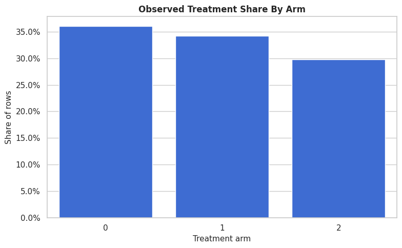
Treatment Share Plot

A simple treatment-share plot helps confirm that all arms have enough data. Multi-arm causal estimation becomes fragile when one arm is rare, especially if the rare arm is concentrated in a narrow covariate region.

fig, ax = plt.subplots(figsize=(8, 5))
arm_counts = multi_df["treatment_arm"].value_counts(normalize=True).rename_axis("treatment_arm").reset_index(name="share")
sns.barplot(data=arm_counts, x="treatment_arm", y="share", color="#2563eb", ax=ax)
ax.yaxis.set_major_formatter(PercentFormatter(1.0))
ax.set_title("Observed Treatment Share By Arm")
ax.set_xlabel("Treatment arm")
ax.set_ylabel("Share of rows")
plt.tight_layout()
fig.savefig(FIGURE_DIR / "10_multi_arm_treatment_share.png", dpi=160, bbox_inches="tight")
plt.show()

All three arms have material support. The arms are not perfectly balanced, but no arm is so rare that the example becomes dominated by sample-size failure.

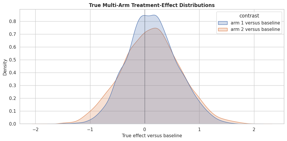
True Arm Effect Distributions

Because this is a teaching dataset, we can inspect the true effect distribution for each active arm. The two distributions are different because each arm helps different row types.

true_effect_long = multi_df[["true_tau_arm_1", "true_tau_arm_2"]].rename(
    columns={"true_tau_arm_1": "arm 1 versus baseline", "true_tau_arm_2": "arm 2 versus baseline"}
).melt(var_name="contrast", value_name="true_effect")

fig, ax = plt.subplots(figsize=(10, 5))
sns.kdeplot(data=true_effect_long, x="true_effect", hue="contrast", fill=True, common_norm=False, alpha=0.25, ax=ax)
ax.axvline(0, color="#111827", linestyle=":", linewidth=1)
ax.set_title("True Multi-Arm Treatment-Effect Distributions")
ax.set_xlabel("True effect versus baseline")
ax.set_ylabel("Density")
plt.tight_layout()
fig.savefig(FIGURE_DIR / "10_multi_arm_true_effect_distributions.png", dpi=160, bbox_inches="tight")
plt.show()

The two arms have overlapping but distinct effect distributions. This is the reason multi-arm learning is not just two separate binary questions; the final decision may require comparing both active arms for the same row.

Naive Arm Differences Versus Truth

This cell computes raw outcome differences between each active arm and the baseline arm, then compares those raw differences with the true average arm effects. The gap is a teaching view of selection bias.

control_mean = multi_df.loc[multi_df["treatment_arm"] == 0, "outcome"].mean()
naive_arm_rows = []
for arm, true_col in [(1, "true_tau_arm_1"), (2, "true_tau_arm_2")]:
    arm_mean = multi_df.loc[multi_df["treatment_arm"] == arm, "outcome"].mean()
    naive_arm_rows.append(
        {
            "contrast": f"arm {arm} versus baseline",
            "raw_outcome_difference": arm_mean - control_mean,
            "true_average_effect": multi_df[true_col].mean(),
            "raw_minus_true": arm_mean - control_mean - multi_df[true_col].mean(),
        }
    )

naive_arm_comparison = pd.DataFrame(naive_arm_rows)
naive_arm_comparison.to_csv(TABLE_DIR / "10_multi_arm_naive_vs_truth.csv", index=False)
display(naive_arm_comparison)

	contrast	raw_outcome_difference	true_average_effect	raw_minus_true
0	arm 1 versus baseline	0.753653	0.135156	0.618497
1	arm 2 versus baseline	0.624697	0.116860	0.507836

The raw differences are not the same as the true average effects. Multi-arm observational data can have selection bias in every active-arm contrast, so each contrast needs adjustment.

Multi-Arm Train-Test Split

We split the multi-arm dataset before fitting the estimator. Stratifying by treatment arm keeps all arms represented in both train and test splits.

multi_feature_cols = [
    "baseline_need",
    "prior_engagement",
    "friction_score",
    "content_affinity",
    "novelty_preference",
    "price_sensitivity",
    "account_tenure",
    "region_risk",
    "high_need_segment",
    "low_friction_segment",
]

multi_train, multi_test = train_test_split(
    multi_df,
    test_size=0.35,
    random_state=202610,
    stratify=multi_df["treatment_arm"],
)
multi_train = multi_train.reset_index(drop=True)
multi_test = multi_test.reset_index(drop=True)

multi_split_summary = pd.DataFrame(
    {
        "split": ["train", "test"],
        "rows": [len(multi_train), len(multi_test)],
        "arm_0_rate": [(multi_train["treatment_arm"] == 0).mean(), (multi_test["treatment_arm"] == 0).mean()],
        "arm_1_rate": [(multi_train["treatment_arm"] == 1).mean(), (multi_test["treatment_arm"] == 1).mean()],
        "arm_2_rate": [(multi_train["treatment_arm"] == 2).mean(), (multi_test["treatment_arm"] == 2).mean()],
        "true_tau_arm_1_mean": [multi_train["true_tau_arm_1"].mean(), multi_test["true_tau_arm_1"].mean()],
        "true_tau_arm_2_mean": [multi_train["true_tau_arm_2"].mean(), multi_test["true_tau_arm_2"].mean()],
    }
)

multi_split_summary.to_csv(TABLE_DIR / "10_multi_arm_train_test_split_summary.csv", index=False)
display(multi_split_summary)

	split	rows	arm_0_rate	arm_1_rate	arm_2_rate	true_tau_arm_1_mean	true_tau_arm_2_mean
0	train	2730	0.360440	0.341758	0.297802	0.130538	0.112445
1	test	1470	0.359864	0.342177	0.297959	0.143733	0.125060

The split keeps treatment shares very similar across train and test. That makes held-out arm-specific diagnostics more stable.

Multi-Arm Model Matrices

This cell extracts the covariate matrix, treatment-arm vector, and outcome vector. Multi-arm treatments stay as integer labels because DRLearner can model the discrete arm assignment process directly.

X_multi_train = multi_train[multi_feature_cols].copy()
X_multi_test = multi_test[multi_feature_cols].copy()
T_multi_train = multi_train["treatment_arm"].to_numpy()
T_multi_test = multi_test["treatment_arm"].to_numpy()
y_multi_train = multi_train["outcome"].to_numpy()
y_multi_test = multi_test["outcome"].to_numpy()
true_tau_1_test = multi_test["true_tau_arm_1"].to_numpy()
true_tau_2_test = multi_test["true_tau_arm_2"].to_numpy()

multi_matrix_summary = pd.DataFrame(
    {
        "object": ["X_multi_train", "X_multi_test", "T_multi_train", "y_multi_train"],
        "shape_or_length": [X_multi_train.shape, X_multi_test.shape, len(T_multi_train), len(y_multi_train)],
        "description": [
            "Observed pre-treatment covariates for multi-arm CATE estimation.",
            "Held-out covariates for evaluating arm-specific effects.",
            "Integer arm labels for the training split.",
            "Observed outcomes for the training split.",
        ],
    }
)

multi_matrix_summary.to_csv(TABLE_DIR / "10_multi_arm_model_matrix_summary.csv", index=False)
display(multi_matrix_summary)

	object	shape_or_length	description
0	X_multi_train	(2730, 10)	Observed pre-treatment covariates for multi-ar...
1	X_multi_test	(1470, 10)	Held-out covariates for evaluating arm-specifi...
2	T_multi_train	2730	Integer arm labels for the training split.
3	y_multi_train	2730	Observed outcomes for the training split.

The treatment vector has three possible values. The estimator will learn the outcome process and the multinomial treatment assignment process from these objects.

Multi-Arm Nuisance Diagnostics

Before fitting DRLearner, we train diagnostic models for arm assignment and outcome prediction. These are not the exact internal nuisance fits, but they tell us whether the observed covariates carry useful signal.

arm_propensity_diagnostic = LogisticRegression(max_iter=1_000)
arm_propensity_diagnostic.fit(X_multi_train, T_multi_train)
arm_propensity_pred = np.clip(arm_propensity_diagnostic.predict_proba(X_multi_test), 1e-4, 1 - 1e-4)

arm_outcome_features_train = X_multi_train.assign(treatment_arm=T_multi_train)
arm_outcome_features_test = X_multi_test.assign(treatment_arm=T_multi_test)
arm_outcome_diagnostic = RandomForestRegressor(
    n_estimators=220,
    min_samples_leaf=20,
    random_state=202611,
    n_jobs=-1,
)
arm_outcome_diagnostic.fit(arm_outcome_features_train, y_multi_train)
arm_outcome_pred = arm_outcome_diagnostic.predict(arm_outcome_features_test)

multi_nuisance_diagnostics = pd.DataFrame(
    [
        {
            "model": "multinomial_arm_model",
            "metric_1": "accuracy",
            "value_1": accuracy_score(T_multi_test, arm_propensity_diagnostic.predict(X_multi_test)),
            "metric_2": "log_loss",
            "value_2": log_loss(T_multi_test, arm_propensity_pred),
        },
        {
            "model": "outcome_model",
            "metric_1": "rmse",
            "value_1": np.sqrt(mean_squared_error(y_multi_test, arm_outcome_pred)),
            "metric_2": "mae",
            "value_2": mean_absolute_error(y_multi_test, arm_outcome_pred),
        },
    ]
)

multi_nuisance_diagnostics.to_csv(TABLE_DIR / "10_multi_arm_nuisance_diagnostics.csv", index=False)
display(multi_nuisance_diagnostics)

	model	metric_1	value_1	metric_2	value_2
0	multinomial_arm_model	accuracy	0.465986	log_loss	1.030364
1	outcome_model	rmse	0.910379	mae	0.716105

The arm model has nontrivial predictive signal, which confirms the observational assignment process is confounded. Doubly robust estimation is useful here because it uses both outcome and treatment-assignment nuisance information.

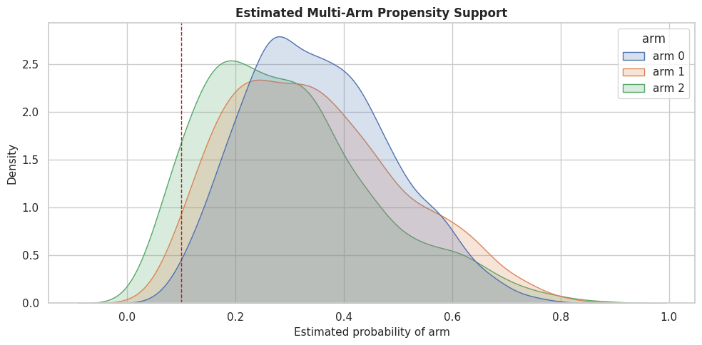
Multi-Arm Propensity Support

For multi-arm treatments, overlap means each arm has a reasonable probability in the regions where we compare arms. This cell summarizes the estimated probability of each arm on held-out rows.

propensity_support = pd.DataFrame(
    arm_propensity_pred,
    columns=["estimated_p_arm_0", "estimated_p_arm_1", "estimated_p_arm_2"],
)
propensity_support_summary = propensity_support.agg(["min", "mean", "median", "max"]).T.reset_index().rename(columns={"index": "propensity"})
propensity_support_summary["share_below_0_10"] = (propensity_support < 0.10).mean().to_numpy()

propensity_support_summary.to_csv(TABLE_DIR / "10_multi_arm_propensity_support_summary.csv", index=False)
display(propensity_support_summary)

	propensity	min	mean	median	max	share_below_0_10
0	estimated_p_arm_0	0.059961	0.355676	0.345325	0.790690	0.007483
1	estimated_p_arm_1	0.030282	0.346332	0.326099	0.830833	0.024490
2	estimated_p_arm_2	0.020873	0.297992	0.273982	0.881861	0.078912

The support summary checks whether any arm has near-zero estimated probability for many rows. When an arm has weak support, its contrast against baseline becomes more fragile.

Propensity Support Plot

The table gives exact values, but the distribution plot makes support problems easier to see. Each curve shows the estimated probability of one arm on held-out rows.

propensity_long = propensity_support.rename(
    columns={
        "estimated_p_arm_0": "arm 0",
        "estimated_p_arm_1": "arm 1",
        "estimated_p_arm_2": "arm 2",
    }
).melt(var_name="arm", value_name="estimated_probability")

fig, ax = plt.subplots(figsize=(10, 5))
sns.kdeplot(data=propensity_long, x="estimated_probability", hue="arm", fill=True, common_norm=False, alpha=0.22, ax=ax)
ax.axvline(0.10, color="#b91c1c", linestyle="--", linewidth=1, label="0.10 support marker")
ax.set_title("Estimated Multi-Arm Propensity Support")
ax.set_xlabel("Estimated probability of arm")
ax.set_ylabel("Density")
plt.tight_layout()
fig.savefig(FIGURE_DIR / "10_multi_arm_propensity_support.png", dpi=160, bbox_inches="tight")
plt.show()

The plot shows whether any treatment arm becomes implausible for large parts of the covariate space. Those regions are where arm-specific effect estimates should be handled carefully.

Fit Multi-Arm DRLearner

DRLearner works well for this section because it is designed for discrete treatments and can use both outcome regression and propensity modeling. We ask it to estimate active-arm effects relative to arm 0.

multi_dr = DRLearner(
    model_propensity=LogisticRegression(max_iter=1_000),
    model_regression=RandomForestRegressor(
        n_estimators=220,
        min_samples_leaf=20,
        random_state=202612,
        n_jobs=-1,
    ),
    model_final=RandomForestRegressor(
        n_estimators=260,
        min_samples_leaf=18,
        random_state=202613,
        n_jobs=-1,
    ),
    cv=3,
    random_state=202614,
)

multi_dr.fit(y_multi_train, T_multi_train, X=X_multi_train)

estimated_tau_arm_1 = multi_dr.effect(X_multi_test, T0=0, T1=1)
estimated_tau_arm_2 = multi_dr.effect(X_multi_test, T0=0, T1=2)
estimated_tau_arm_2_vs_1 = estimated_tau_arm_2 - estimated_tau_arm_1

print(f"Mean estimated effect, arm 1 versus baseline: {estimated_tau_arm_1.mean():.4f}")
print(f"Mean estimated effect, arm 2 versus baseline: {estimated_tau_arm_2.mean():.4f}")
print(f"Mean estimated effect, arm 2 versus arm 1: {estimated_tau_arm_2_vs_1.mean():.4f}")

Mean estimated effect, arm 1 versus baseline: 0.1223
Mean estimated effect, arm 2 versus baseline: 0.0906
Mean estimated effect, arm 2 versus arm 1: -0.0317

The estimator returns one contrast at a time. Arm 2 versus arm 1 can be formed by subtracting the two baseline-relative estimates because both effects are measured against the same reference arm.

Multi-Arm CATE Recovery

With synthetic data, we can compare estimated arm-specific CATEs with the true arm-specific effects. This is a teaching diagnostic for whether the estimator learned the right heterogeneity pattern.

multi_eval = multi_test[multi_feature_cols + ["treatment_arm", "outcome", "true_tau_arm_1", "true_tau_arm_2", "true_best_arm", "true_best_gain"]].copy()
multi_eval["estimated_tau_arm_1"] = estimated_tau_arm_1
multi_eval["estimated_tau_arm_2"] = estimated_tau_arm_2
multi_eval["estimated_tau_arm_2_vs_1"] = estimated_tau_arm_2_vs_1
multi_eval["estimated_best_arm"] = np.argmax(
    np.column_stack([np.zeros(len(multi_eval)), estimated_tau_arm_1, estimated_tau_arm_2]),
    axis=1,
)
multi_eval["estimated_best_gain"] = np.maximum.reduce([np.zeros(len(multi_eval)), estimated_tau_arm_1, estimated_tau_arm_2])

multi_cate_recovery = pd.DataFrame(
    [
        {
            "contrast": "arm 1 versus baseline",
            "true_mean_effect": true_tau_1_test.mean(),
            "estimated_mean_effect": estimated_tau_arm_1.mean(),
            "rmse": np.sqrt(mean_squared_error(true_tau_1_test, estimated_tau_arm_1)),
            "mae": mean_absolute_error(true_tau_1_test, estimated_tau_arm_1),
            "correlation": np.corrcoef(true_tau_1_test, estimated_tau_arm_1)[0, 1],
        },
        {
            "contrast": "arm 2 versus baseline",
            "true_mean_effect": true_tau_2_test.mean(),
            "estimated_mean_effect": estimated_tau_arm_2.mean(),
            "rmse": np.sqrt(mean_squared_error(true_tau_2_test, estimated_tau_arm_2)),
            "mae": mean_absolute_error(true_tau_2_test, estimated_tau_arm_2),
            "correlation": np.corrcoef(true_tau_2_test, estimated_tau_arm_2)[0, 1],
        },
    ]
)

multi_cate_recovery.to_csv(TABLE_DIR / "10_multi_arm_cate_recovery.csv", index=False)
multi_eval.to_csv(TABLE_DIR / "10_multi_arm_heldout_effects.csv", index=False)
display(multi_cate_recovery)

	contrast	true_mean_effect	estimated_mean_effect	rmse	mae	correlation
0	arm 1 versus baseline	0.143733	0.122305	0.335129	0.264473	0.792277
1	arm 2 versus baseline	0.125060	0.090606	0.409347	0.307220	0.758176

The recovery table gives a contrast-by-contrast view. In multi-arm settings, one arm can be estimated well while another is weaker, especially if support differs across arms.

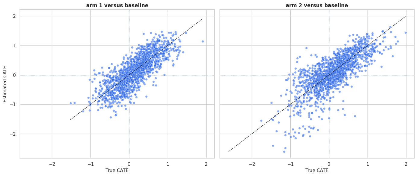
Multi-Arm Recovery Plot

This plot puts the two active-arm recovery patterns side by side. Each point is a held-out row, and the diagonal line marks perfect CATE recovery.

plot_recovery = pd.concat(
    [
        pd.DataFrame({"true_effect": true_tau_1_test, "estimated_effect": estimated_tau_arm_1, "contrast": "arm 1 versus baseline"}),
        pd.DataFrame({"true_effect": true_tau_2_test, "estimated_effect": estimated_tau_arm_2, "contrast": "arm 2 versus baseline"}),
    ],
    ignore_index=True,
)

fig, axes = plt.subplots(1, 2, figsize=(14, 6), sharex=True, sharey=True)
for ax, contrast in zip(axes, plot_recovery["contrast"].unique()):
    subset = plot_recovery[plot_recovery["contrast"] == contrast]
    sns.scatterplot(data=subset, x="true_effect", y="estimated_effect", alpha=0.55, s=28, color="#2563eb", ax=ax)
    lims = [min(subset["true_effect"].min(), subset["estimated_effect"].min()), max(subset["true_effect"].max(), subset["estimated_effect"].max())]
    ax.plot(lims, lims, color="#111827", linestyle="--", linewidth=1)
    ax.axhline(0, color="#64748b", linestyle=":", linewidth=1)
    ax.axvline(0, color="#64748b", linestyle=":", linewidth=1)
    ax.set_title(contrast)
    ax.set_xlabel("True CATE")
    ax.set_ylabel("Estimated CATE")
plt.tight_layout()
fig.savefig(FIGURE_DIR / "10_multi_arm_cate_recovery.png", dpi=160, bbox_inches="tight")
plt.show()

The side-by-side view makes arm-specific strengths and weaknesses visible. A good multi-arm model should recover not only average effects, but also the ordering of arms within rows.

Estimated Best-Arm Policy

Multi-arm CATE estimates become useful when we compare arms for each row. This cell chooses the estimated best arm and compares it with the oracle best arm from the synthetic truth.

best_arm_accuracy = accuracy_score(multi_eval["true_best_arm"], multi_eval["estimated_best_arm"])
policy_gain_table = pd.DataFrame(
    [
        {
            "policy": "observed historical assignment",
            "mean_true_gain": np.select(
                [multi_eval["treatment_arm"] == 1, multi_eval["treatment_arm"] == 2],
                [multi_eval["true_tau_arm_1"], multi_eval["true_tau_arm_2"]],
                default=0.0,
            ).mean(),
            "arm_0_rate": (multi_eval["treatment_arm"] == 0).mean(),
            "arm_1_rate": (multi_eval["treatment_arm"] == 1).mean(),
            "arm_2_rate": (multi_eval["treatment_arm"] == 2).mean(),
        },
        {
            "policy": "estimated best arm",
            "mean_true_gain": np.select(
                [multi_eval["estimated_best_arm"] == 1, multi_eval["estimated_best_arm"] == 2],
                [multi_eval["true_tau_arm_1"], multi_eval["true_tau_arm_2"]],
                default=0.0,
            ).mean(),
            "arm_0_rate": (multi_eval["estimated_best_arm"] == 0).mean(),
            "arm_1_rate": (multi_eval["estimated_best_arm"] == 1).mean(),
            "arm_2_rate": (multi_eval["estimated_best_arm"] == 2).mean(),
        },
        {
            "policy": "oracle best arm",
            "mean_true_gain": multi_eval["true_best_gain"].mean(),
            "arm_0_rate": (multi_eval["true_best_arm"] == 0).mean(),
            "arm_1_rate": (multi_eval["true_best_arm"] == 1).mean(),
            "arm_2_rate": (multi_eval["true_best_arm"] == 2).mean(),
        },
    ]
)

best_arm_summary = pd.DataFrame(
    {
        "metric": ["best_arm_accuracy", "estimated_policy_regret_vs_oracle"],
        "value": [
            best_arm_accuracy,
            policy_gain_table.loc[policy_gain_table["policy"] == "oracle best arm", "mean_true_gain"].iloc[0]
            - policy_gain_table.loc[policy_gain_table["policy"] == "estimated best arm", "mean_true_gain"].iloc[0],
        ],
    }
)

policy_gain_table.to_csv(TABLE_DIR / "10_multi_arm_policy_gain_table.csv", index=False)
best_arm_summary.to_csv(TABLE_DIR / "10_multi_arm_best_arm_summary.csv", index=False)
display(best_arm_summary)
display(policy_gain_table)

	metric	value
0	best_arm_accuracy	0.636735
1	estimated_policy_regret_vs_oracle	0.062944

	policy	mean_true_gain	arm_0_rate	arm_1_rate	arm_2_rate
0	observed historical assignment	0.194026	0.359864	0.342177	0.297959
1	estimated best arm	0.361965	0.212925	0.406803	0.380272
2	oracle best arm	0.424909	0.000000	0.523810	0.476190

The estimated policy can improve over historical assignment if the arm-specific estimates rank arms well. The gap to the oracle is regret: value left on the table because the model does not know the true effects perfectly.

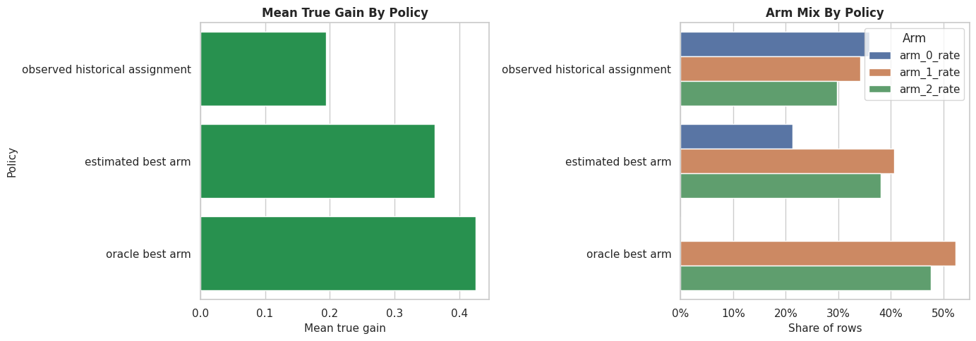
Best-Arm Policy Plot

The table is precise, but a plot makes the policy comparison easier to communicate. We show both average true gain and how often each policy uses each arm.

fig, axes = plt.subplots(1, 2, figsize=(14, 5))

sns.barplot(data=policy_gain_table, x="mean_true_gain", y="policy", color="#16a34a", ax=axes[0])
axes[0].set_title("Mean True Gain By Policy")
axes[0].set_xlabel("Mean true gain")
axes[0].set_ylabel("Policy")

arm_mix = policy_gain_table.melt(
    id_vars="policy",
    value_vars=["arm_0_rate", "arm_1_rate", "arm_2_rate"],
    var_name="arm",
    value_name="rate",
)
sns.barplot(data=arm_mix, x="rate", y="policy", hue="arm", ax=axes[1])
axes[1].set_title("Arm Mix By Policy")
axes[1].set_xlabel("Share of rows")
axes[1].set_ylabel("")
axes[1].xaxis.set_major_formatter(PercentFormatter(1.0))
axes[1].legend(title="Arm")

plt.tight_layout()
fig.savefig(FIGURE_DIR / "10_multi_arm_policy_comparison.png", dpi=160, bbox_inches="tight")
plt.show()

The policy view is the payoff of multi-arm estimation. We are no longer asking whether treatment works in general; we are asking which treatment works best for which rows.

Segment-Level Arm Effects

A segment summary helps explain the policy in human-readable terms. Here we group by need and novelty preference, then compare true and estimated arm effects within each segment.

segment_multi = multi_eval.copy()
segment_multi["need_segment"] = np.where(segment_multi["baseline_need"] > segment_multi["baseline_need"].median(), "higher need", "lower need")
segment_multi["novelty_segment"] = np.where(segment_multi["novelty_preference"] > segment_multi["novelty_preference"].median(), "higher novelty", "lower novelty")

multi_segment_summary = (
    segment_multi.groupby(["need_segment", "novelty_segment"], observed=True)
    .agg(
        rows=("outcome", "size"),
        true_tau_arm_1_mean=("true_tau_arm_1", "mean"),
        estimated_tau_arm_1_mean=("estimated_tau_arm_1", "mean"),
        true_tau_arm_2_mean=("true_tau_arm_2", "mean"),
        estimated_tau_arm_2_mean=("estimated_tau_arm_2", "mean"),
        estimated_arm_1_rate=("estimated_best_arm", lambda s: np.mean(s == 1)),
        estimated_arm_2_rate=("estimated_best_arm", lambda s: np.mean(s == 2)),
    )
    .reset_index()
)

multi_segment_summary.to_csv(TABLE_DIR / "10_multi_arm_segment_summary.csv", index=False)
display(multi_segment_summary)

	need_segment	novelty_segment	rows	true_tau_arm_1_mean	estimated_tau_arm_1_mean	true_tau_arm_2_mean	estimated_tau_arm_2_mean	estimated_arm_1_rate	estimated_arm_2_rate
0	higher need	higher novelty	383	0.445799	0.488384	0.445562	0.389181	0.566580	0.381201
1	higher need	lower novelty	352	0.424514	0.435947	-0.174147	-0.152231	0.758523	0.139205
2	lower need	higher novelty	352	-0.139074	-0.142376	0.464974	0.415551	0.102273	0.747159
3	lower need	lower novelty	383	-0.156471	-0.288772	-0.232856	-0.283431	0.203655	0.263708

The segment table shows why the two arms are different. Guided personalization tends to align with need and engagement, while the exploration arm is designed to align with novelty preference and lower friction.

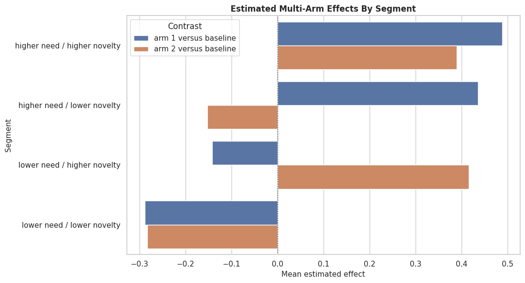
Segment Arm-Effect Plot

The next plot compares estimated active-arm effects by segment. This is often more digestible than individual CATE scatterplots.

segment_plot = multi_segment_summary.copy()
segment_plot["segment"] = segment_plot["need_segment"] + " / " + segment_plot["novelty_segment"]
segment_effect_plot = segment_plot.melt(
    id_vars="segment",
    value_vars=["estimated_tau_arm_1_mean", "estimated_tau_arm_2_mean"],
    var_name="contrast",
    value_name="estimated_effect",
)
segment_effect_plot["contrast"] = segment_effect_plot["contrast"].map(
    {
        "estimated_tau_arm_1_mean": "arm 1 versus baseline",
        "estimated_tau_arm_2_mean": "arm 2 versus baseline",
    }
)

fig, ax = plt.subplots(figsize=(11, 6))
sns.barplot(data=segment_effect_plot, x="estimated_effect", y="segment", hue="contrast", ax=ax)
ax.axvline(0, color="#111827", linestyle=":", linewidth=1)
ax.set_title("Estimated Multi-Arm Effects By Segment")
ax.set_xlabel("Mean estimated effect")
ax.set_ylabel("Segment")
ax.legend(title="Contrast")
plt.tight_layout()
fig.savefig(FIGURE_DIR / "10_multi_arm_segment_effects.png", dpi=160, bbox_inches="tight")
plt.show()

The segment plot makes it clear that multi-arm estimation is about matching rows to arms, not simply finding one universally best intervention.

Part B: Continuous Treatments

Now we move from choosing among discrete arms to estimating the effect of a continuous dose. The treatment might represent intensity, minutes, discount size, number of recommendations, support hours, or any other continuous amount.

Continuous Treatment Estimand

For continuous treatments, the main estimand is often a marginal effect: the expected outcome change for a one-unit increase in treatment intensity, conditional on covariates. We can also ask for a finite contrast such as increasing dose from 0.5 to 1.5.

continuous_estimand_table = pd.DataFrame(
    [
        {
            "quantity": "Marginal dose effect",
            "notation": "d E[Y(t) | X] / dt",
            "plain_language": "Outcome change for a small one-unit increase in dose at a covariate profile.",
            "econml_call": "est.const_marginal_effect(X)",
        },
        {
            "quantity": "Finite dose contrast",
            "notation": "E[Y(t=b) - Y(t=a) | X]",
            "plain_language": "Outcome change when moving from dose a to dose b.",
            "econml_call": "est.effect(X, T0=a, T1=b)",
        },
        {
            "quantity": "Dose support check",
            "notation": "Observed T distribution by segment",
            "plain_language": "Whether the data contain enough dose variation to support the contrast.",
            "econml_call": "Diagnostic outside the estimator",
        },
    ]
)

continuous_estimand_table.to_csv(TABLE_DIR / "10_continuous_estimand_table.csv", index=False)
display(continuous_estimand_table)

	quantity	notation	plain_language	econml_call
0	Marginal dose effect	d E[Y(t) | X] / dt	Outcome change for a small one-unit increase i...	est.const_marginal_effect(X)
1	Finite dose contrast	E[Y(t=b) - Y(t=a) | X]	Outcome change when moving from dose a to dose b.	est.effect(X, T0=a, T1=b)
2	Dose support check	Observed T distribution by segment	Whether the data contain enough dose variation...	Diagnostic outside the estimator

Continuous treatments make support especially important. A one-unit contrast is easier to defend when the observed data contain comparable rows with a wide range of treatment intensities.

Continuous-Dose Teaching Data

This cell creates a continuous treatment intensity. The true outcome model is linear in the dose, but the slope varies across covariates. That makes LinearDML a good teaching estimator because it estimates heterogeneous marginal effects.

def true_dose_slope(frame):
    """Ground-truth marginal effect of one additional treatment-intensity unit."""
    return (
        0.34
        + 0.28 * frame["baseline_need"]
        + 0.18 * frame["content_affinity"]
        - 0.22 * frame["friction_score"]
        - 0.24 * frame["price_sensitivity"]
        + 0.16 * frame["high_capacity_segment"]
        - 0.14 * frame["region_risk"]
    )


n_cont = 3_800
baseline_need = rng.normal(0, 1, size=n_cont)
prior_engagement = rng.normal(0, 1, size=n_cont)
friction_score = rng.normal(0, 1, size=n_cont)
content_affinity = rng.normal(0, 1, size=n_cont)
price_sensitivity = rng.beta(2.1, 3.4, size=n_cont)
capacity_score = rng.normal(0, 1, size=n_cont)
account_tenure = rng.gamma(shape=3.0, scale=15.0, size=n_cont)
region_risk = rng.binomial(1, 0.27, size=n_cont)
high_capacity_segment = (capacity_score > 0.35).astype(int)

continuous_features = pd.DataFrame(
    {
        "baseline_need": baseline_need,
        "prior_engagement": prior_engagement,
        "friction_score": friction_score,
        "content_affinity": content_affinity,
        "price_sensitivity": price_sensitivity,
        "capacity_score": capacity_score,
        "account_tenure": account_tenure,
        "region_risk": region_risk,
        "high_capacity_segment": high_capacity_segment,
    }
)

true_slope = true_dose_slope(continuous_features)
continuous_treatment = (
    1.20
    + 0.42 * baseline_need
    + 0.35 * prior_engagement
    - 0.32 * friction_score
    + 0.25 * capacity_score
    - 0.28 * price_sensitivity
    + 0.18 * content_affinity
    + rng.normal(0, 0.70, size=n_cont)
)
continuous_treatment = np.clip(continuous_treatment, -1.5, 3.5)

base_continuous_outcome = (
    1.00
    + 0.48 * baseline_need
    + 0.40 * prior_engagement
    - 0.28 * friction_score
    + 0.24 * content_affinity
    - 0.18 * price_sensitivity
    + 0.12 * np.log1p(account_tenure)
    - 0.16 * region_risk
)
continuous_outcome = base_continuous_outcome + true_slope * continuous_treatment + rng.normal(0, 0.72, size=n_cont)

continuous_df = continuous_features.assign(
    treatment_intensity=continuous_treatment,
    outcome=continuous_outcome,
    true_marginal_effect=true_slope,
    true_effect_0_to_1=true_slope,
    true_effect_0_to_2=2 * true_slope,
)

continuous_df.to_csv(TABLE_DIR / "10_continuous_teaching_data.csv", index=False)
continuous_df.head()

	baseline_need	prior_engagement	friction_score	content_affinity	price_sensitivity	capacity_score	account_tenure	region_risk	high_capacity_segment	treatment_intensity	outcome	true_marginal_effect	true_effect_0_to_1	true_effect_0_to_2
0	0.231017	-1.124913	0.230528	-0.138457	0.718611	-1.603517	20.039041	0	0	0.791611	0.747094	0.156580	0.156580	0.313159
1	0.133910	1.097815	-1.259895	0.084472	0.523923	-0.025354	54.492049	1	0	2.056314	3.690250	0.404135	0.404135	0.808271
2	0.119791	-0.673244	-1.596195	2.248898	0.285746	-0.381237	63.664264	0	0	1.978979	5.546482	1.060927	1.060927	2.121854
3	-0.870117	0.008350	0.136661	-0.474915	0.229955	-0.352024	27.547564	0	0	0.977252	0.402511	-0.074372	-0.074372	-0.148744
4	0.181832	0.645825	1.498643	1.464674	0.181864	0.330741	52.486607	0	0	2.077669	1.723572	0.281206	0.281206	0.562411

The treatment is a continuous intensity, not a binary indicator. The truth columns show the marginal effect and finite contrasts that we will use to evaluate the estimator.

Continuous Field Dictionary

The continuous-treatment example uses a separate field dictionary so the dose variable is clearly distinguished from the outcome and effect columns.

continuous_field_dictionary = pd.DataFrame(
    [
        ("baseline_need", "Observed covariate", "Pre-treatment need or demand signal."),
        ("prior_engagement", "Observed covariate", "Historical engagement before treatment intensity is assigned."),
        ("friction_score", "Observed covariate", "Higher values indicate more friction."),
        ("content_affinity", "Observed covariate", "Match between row and content or offer."),
        ("price_sensitivity", "Observed covariate", "Sensitivity to cost or inconvenience."),
        ("capacity_score", "Observed covariate", "Ability to absorb more treatment intensity."),
        ("account_tenure", "Observed covariate", "Age of the relationship in weeks."),
        ("region_risk", "Observed covariate", "Binary marker for lower baseline outcome regions."),
        ("high_capacity_segment", "Observed covariate", "Binary segment derived from capacity score."),
        ("treatment_intensity", "Treatment", "Continuous treatment dose or intensity."),
        ("outcome", "Outcome", "Observed post-treatment outcome."),
        ("true_marginal_effect", "Teaching-only truth", "True one-unit dose effect for each row."),
        ("true_effect_0_to_1", "Teaching-only truth", "True effect of increasing dose from 0 to 1."),
        ("true_effect_0_to_2", "Teaching-only truth", "True effect of increasing dose from 0 to 2."),
    ],
    columns=["field", "role", "description"],
)

continuous_field_dictionary.to_csv(TABLE_DIR / "10_continuous_field_dictionary.csv", index=False)
display(continuous_field_dictionary)

	field	role	description
0	baseline_need	Observed covariate	Pre-treatment need or demand signal.
1	prior_engagement	Observed covariate	Historical engagement before treatment intensi...
2	friction_score	Observed covariate	Higher values indicate more friction.
3	content_affinity	Observed covariate	Match between row and content or offer.
4	price_sensitivity	Observed covariate	Sensitivity to cost or inconvenience.
5	capacity_score	Observed covariate	Ability to absorb more treatment intensity.
6	account_tenure	Observed covariate	Age of the relationship in weeks.
7	region_risk	Observed covariate	Binary marker for lower baseline outcome regions.
8	high_capacity_segment	Observed covariate	Binary segment derived from capacity score.
9	treatment_intensity	Treatment	Continuous treatment dose or intensity.
10	outcome	Outcome	Observed post-treatment outcome.
11	true_marginal_effect	Teaching-only truth	True one-unit dose effect for each row.
12	true_effect_0_to_1	Teaching-only truth	True effect of increasing dose from 0 to 1.
13	true_effect_0_to_2	Teaching-only truth	True effect of increasing dose from 0 to 2.

The treatment column is numeric and ordered. That changes the modeling goal from estimating arm contrasts to estimating a slope or dose contrast.

Continuous Treatment Summary

This cell checks the distribution of treatment intensity, the outcome, and the true marginal effect. We also look at the correlation between treatment intensity and covariates, because confounded continuous treatments are assigned more intensely to some row types.

continuous_basic_summary = pd.DataFrame(
    {
        "metric": [
            "rows",
            "columns",
            "treatment_intensity_mean",
            "treatment_intensity_std",
            "treatment_intensity_min",
            "treatment_intensity_max",
            "outcome_mean",
            "true_marginal_effect_mean",
            "true_marginal_effect_std",
            "share_positive_marginal_effect",
        ],
        "value": [
            len(continuous_df),
            continuous_df.shape[1],
            continuous_df["treatment_intensity"].mean(),
            continuous_df["treatment_intensity"].std(),
            continuous_df["treatment_intensity"].min(),
            continuous_df["treatment_intensity"].max(),
            continuous_df["outcome"].mean(),
            continuous_df["true_marginal_effect"].mean(),
            continuous_df["true_marginal_effect"].std(),
            (continuous_df["true_marginal_effect"] > 0).mean(),
        ],
    }
)

continuous_basic_summary.to_csv(TABLE_DIR / "10_continuous_basic_summary.csv", index=False)
display(continuous_basic_summary)

	metric	value
0	rows	3800.000000
1	columns	14.000000
2	treatment_intensity_mean	1.083585
3	treatment_intensity_std	0.992498
4	treatment_intensity_min	-1.500000
5	treatment_intensity_max	3.500000
6	outcome_mean	1.846560
7	true_marginal_effect_mean	0.268117
8	true_marginal_effect_std	0.415548
9	share_positive_marginal_effect	0.738158

The treatment has broad support and the true marginal effect varies across rows. That gives LinearDML a meaningful heterogeneity problem to solve.

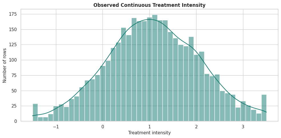
Continuous Treatment Distribution

A continuous treatment should be inspected like a numeric exposure. The histogram shows whether the dose has enough variation and whether clipping has created large spikes at the boundaries.

fig, ax = plt.subplots(figsize=(10, 5))
sns.histplot(continuous_df["treatment_intensity"], bins=45, kde=True, color="#0f766e", ax=ax)
ax.set_title("Observed Continuous Treatment Intensity")
ax.set_xlabel("Treatment intensity")
ax.set_ylabel("Number of rows")
plt.tight_layout()
fig.savefig(FIGURE_DIR / "10_continuous_treatment_distribution.png", dpi=160, bbox_inches="tight")
plt.show()

The treatment distribution is continuous with useful spread. Boundary mass would make some dose contrasts less credible, so it is worth checking before model fitting.

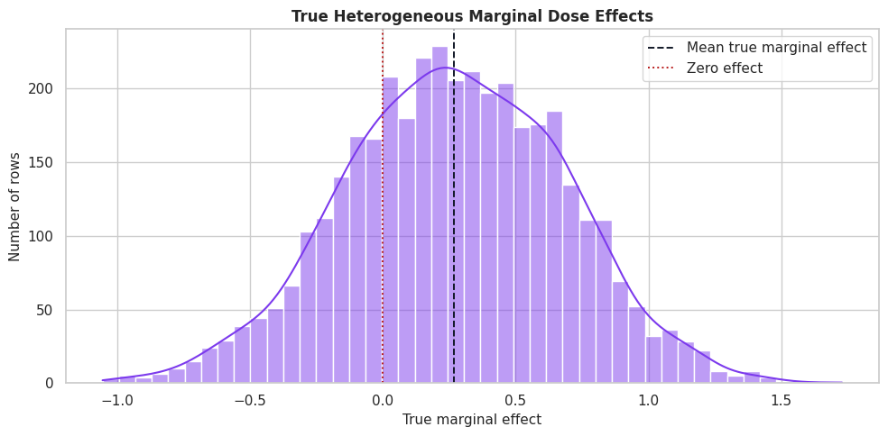
True Marginal Effect Distribution

This plot shows the true heterogeneous slope. In real data, this distribution is unknown; here it gives us a target for evaluating the estimated marginal effects.

fig, ax = plt.subplots(figsize=(10, 5))
sns.histplot(continuous_df["true_marginal_effect"], bins=45, kde=True, color="#7c3aed", ax=ax)
ax.axvline(continuous_df["true_marginal_effect"].mean(), color="#111827", linestyle="--", linewidth=1.4, label="Mean true marginal effect")
ax.axvline(0, color="#b91c1c", linestyle=":", linewidth=1.4, label="Zero effect")
ax.set_title("True Heterogeneous Marginal Dose Effects")
ax.set_xlabel("True marginal effect")
ax.set_ylabel("Number of rows")
ax.legend()
plt.tight_layout()
fig.savefig(FIGURE_DIR / "10_continuous_true_marginal_effect_distribution.png", dpi=160, bbox_inches="tight")
plt.show()

The marginal effect is positive for many rows but not all rows. A dose-increase policy should therefore be selective rather than assuming more intensity is always better.

Dose Support By Segment

For continuous treatments, support means having dose variation within the segments where we want to estimate effects. This cell summarizes dose distributions by high-capacity segment.

dose_support_by_segment = (
    continuous_df.assign(capacity_segment=np.where(continuous_df["high_capacity_segment"] == 1, "high capacity", "regular capacity"))
    .groupby("capacity_segment", observed=True)
    .agg(
        rows=("treatment_intensity", "size"),
        dose_mean=("treatment_intensity", "mean"),
        dose_std=("treatment_intensity", "std"),
        dose_min=("treatment_intensity", "min"),
        dose_p10=("treatment_intensity", lambda s: s.quantile(0.10)),
        dose_p90=("treatment_intensity", lambda s: s.quantile(0.90)),
        dose_max=("treatment_intensity", "max"),
        true_marginal_effect_mean=("true_marginal_effect", "mean"),
    )
    .reset_index()
)

dose_support_by_segment.to_csv(TABLE_DIR / "10_continuous_dose_support_by_segment.csv", index=False)
display(dose_support_by_segment)

	capacity_segment	rows	dose_mean	dose_std	dose_min	dose_p10	dose_p90	dose_max	true_marginal_effect_mean
0	high capacity	1377	1.332073	0.973032	-1.5	0.115144	2.648401	3.5	0.371357
1	regular capacity	2423	0.942369	0.975776	-1.5	-0.338502	2.204940	3.5	0.209445

Both segments have variation in treatment intensity. If one segment had almost no dose variation, its marginal-effect estimate would be much harder to trust.

Continuous Train-Test Split

We split the continuous-treatment data before fitting the model. Because the treatment is continuous, we stratify on a binned version of dose to keep dose ranges represented in both train and test splits.

continuous_feature_cols = [
    "baseline_need",
    "prior_engagement",
    "friction_score",
    "content_affinity",
    "price_sensitivity",
    "capacity_score",
    "account_tenure",
    "region_risk",
    "high_capacity_segment",
]

dose_bins = pd.qcut(continuous_df["treatment_intensity"], q=5, labels=False, duplicates="drop")
continuous_train, continuous_test = train_test_split(
    continuous_df,
    test_size=0.35,
    random_state=202611,
    stratify=dose_bins,
)
continuous_train = continuous_train.reset_index(drop=True)
continuous_test = continuous_test.reset_index(drop=True)

continuous_split_summary = pd.DataFrame(
    {
        "split": ["train", "test"],
        "rows": [len(continuous_train), len(continuous_test)],
        "dose_mean": [continuous_train["treatment_intensity"].mean(), continuous_test["treatment_intensity"].mean()],
        "dose_std": [continuous_train["treatment_intensity"].std(), continuous_test["treatment_intensity"].std()],
        "outcome_mean": [continuous_train["outcome"].mean(), continuous_test["outcome"].mean()],
        "true_marginal_effect_mean": [continuous_train["true_marginal_effect"].mean(), continuous_test["true_marginal_effect"].mean()],
    }
)

continuous_split_summary.to_csv(TABLE_DIR / "10_continuous_train_test_split_summary.csv", index=False)
display(continuous_split_summary)

	split	rows	dose_mean	dose_std	outcome_mean	true_marginal_effect_mean
0	train	2470	1.082995	0.999654	1.865068	0.271968
1	test	1330	1.084682	0.979441	1.812190	0.260965

The train and test splits have similar dose and true-effect distributions. That keeps held-out marginal-effect diagnostics meaningful.

Continuous Model Matrices

This cell extracts the covariates, continuous treatment vector, and outcome vector for LinearDML. Unlike the multi-arm section, T is numeric and continuous.

X_cont_train = continuous_train[continuous_feature_cols].copy()
X_cont_test = continuous_test[continuous_feature_cols].copy()
T_cont_train = continuous_train["treatment_intensity"].to_numpy()
T_cont_test = continuous_test["treatment_intensity"].to_numpy()
y_cont_train = continuous_train["outcome"].to_numpy()
y_cont_test = continuous_test["outcome"].to_numpy()
true_slope_test = continuous_test["true_marginal_effect"].to_numpy()

continuous_matrix_summary = pd.DataFrame(
    {
        "object": ["X_cont_train", "X_cont_test", "T_cont_train", "y_cont_train"],
        "shape_or_length": [X_cont_train.shape, X_cont_test.shape, len(T_cont_train), len(y_cont_train)],
        "description": [
            "Observed pre-treatment covariates.",
            "Held-out covariates for marginal-effect evaluation.",
            "Continuous treatment intensity for training rows.",
            "Observed outcomes for training rows.",
        ],
    }
)

continuous_matrix_summary.to_csv(TABLE_DIR / "10_continuous_model_matrix_summary.csv", index=False)
display(continuous_matrix_summary)

	object	shape_or_length	description
0	X_cont_train	(2470, 9)	Observed pre-treatment covariates.
1	X_cont_test	(1330, 9)	Held-out covariates for marginal-effect evalua...
2	T_cont_train	2470	Continuous treatment intensity for training rows.
3	y_cont_train	2470	Observed outcomes for training rows.

The continuous treatment vector has the same length as the outcome vector, but its values are real-valued doses rather than treatment-arm labels.

Continuous Nuisance Diagnostics

LinearDML residualizes both the outcome and the continuous treatment. This diagnostic cell checks whether observed covariates predict the treatment intensity and outcome reasonably well.

dose_model_diagnostic = RandomForestRegressor(
    n_estimators=220,
    min_samples_leaf=20,
    random_state=202615,
    n_jobs=-1,
)
dose_model_diagnostic.fit(X_cont_train, T_cont_train)
dose_pred = dose_model_diagnostic.predict(X_cont_test)

continuous_outcome_features_train = X_cont_train.assign(treatment_intensity=T_cont_train)
continuous_outcome_features_test = X_cont_test.assign(treatment_intensity=T_cont_test)
continuous_outcome_diagnostic = RandomForestRegressor(
    n_estimators=220,
    min_samples_leaf=20,
    random_state=202616,
    n_jobs=-1,
)
continuous_outcome_diagnostic.fit(continuous_outcome_features_train, y_cont_train)
continuous_outcome_pred = continuous_outcome_diagnostic.predict(continuous_outcome_features_test)

continuous_nuisance_diagnostics = pd.DataFrame(
    [
        {
            "model": "dose_model",
            "metric_1": "rmse",
            "value_1": np.sqrt(mean_squared_error(T_cont_test, dose_pred)),
            "metric_2": "mae",
            "value_2": mean_absolute_error(T_cont_test, dose_pred),
        },
        {
            "model": "outcome_model",
            "metric_1": "rmse",
            "value_1": np.sqrt(mean_squared_error(y_cont_test, continuous_outcome_pred)),
            "metric_2": "mae",
            "value_2": mean_absolute_error(y_cont_test, continuous_outcome_pred),
        },
    ]
)

continuous_nuisance_diagnostics.to_csv(TABLE_DIR / "10_continuous_nuisance_diagnostics.csv", index=False)
display(continuous_nuisance_diagnostics)

	model	metric_1	value_1	metric_2	value_2
0	dose_model	rmse	0.738349	mae	0.592988
1	outcome_model	rmse	0.884495	mae	0.701308

The dose model captures confounding in the treatment intensity. That is exactly the structure DML is designed to handle: remove predictable treatment and outcome components, then estimate the residualized treatment effect.

Fit LinearDML For Continuous Treatment

LinearDML estimates a CATE function that is linear in the treatment but can vary with covariates. In this synthetic data, the outcome is linear in dose with a heterogeneous slope, so the estimator is aligned with the teaching setup.

continuous_dml = LinearDML(
    model_y=RandomForestRegressor(
        n_estimators=240,
        min_samples_leaf=20,
        random_state=202617,
        n_jobs=-1,
    ),
    model_t=RandomForestRegressor(
        n_estimators=240,
        min_samples_leaf=20,
        random_state=202618,
        n_jobs=-1,
    ),
    cv=3,
    random_state=202619,
)

continuous_dml.fit(y_cont_train, T_cont_train, X=X_cont_train, inference="statsmodels")

estimated_marginal_effect = np.ravel(continuous_dml.const_marginal_effect(X_cont_test))
estimated_effect_0_to_1 = np.ravel(continuous_dml.effect(X_cont_test, T0=0, T1=1))
estimated_effect_0_to_2 = np.ravel(continuous_dml.effect(X_cont_test, T0=0, T1=2))

print(f"Mean estimated marginal effect: {estimated_marginal_effect.mean():.4f}")
print(f"Mean true marginal effect: {true_slope_test.mean():.4f}")

Mean estimated marginal effect: 0.4192
Mean true marginal effect: 0.2610

For a linear-in-dose treatment model, the one-unit effect from effect(X, T0=0, T1=1) should match the marginal effect. The two-unit contrast should be roughly twice the marginal effect.

Continuous Effect Recovery

This cell compares estimated marginal effects and finite dose contrasts with the synthetic truth. These recovery metrics are teaching diagnostics that would not be available in real observational data.

continuous_eval = continuous_test[continuous_feature_cols + ["treatment_intensity", "outcome", "true_marginal_effect", "true_effect_0_to_1", "true_effect_0_to_2"]].copy()
continuous_eval["estimated_marginal_effect"] = estimated_marginal_effect
continuous_eval["estimated_effect_0_to_1"] = estimated_effect_0_to_1
continuous_eval["estimated_effect_0_to_2"] = estimated_effect_0_to_2

continuous_recovery = pd.DataFrame(
    [
        {
            "quantity": "marginal effect",
            "true_mean": continuous_eval["true_marginal_effect"].mean(),
            "estimated_mean": continuous_eval["estimated_marginal_effect"].mean(),
            "rmse": np.sqrt(mean_squared_error(continuous_eval["true_marginal_effect"], continuous_eval["estimated_marginal_effect"])),
            "mae": mean_absolute_error(continuous_eval["true_marginal_effect"], continuous_eval["estimated_marginal_effect"]),
            "correlation": np.corrcoef(continuous_eval["true_marginal_effect"], continuous_eval["estimated_marginal_effect"])[0, 1],
        },
        {
            "quantity": "effect from dose 0 to 1",
            "true_mean": continuous_eval["true_effect_0_to_1"].mean(),
            "estimated_mean": continuous_eval["estimated_effect_0_to_1"].mean(),
            "rmse": np.sqrt(mean_squared_error(continuous_eval["true_effect_0_to_1"], continuous_eval["estimated_effect_0_to_1"])),
            "mae": mean_absolute_error(continuous_eval["true_effect_0_to_1"], continuous_eval["estimated_effect_0_to_1"]),
            "correlation": np.corrcoef(continuous_eval["true_effect_0_to_1"], continuous_eval["estimated_effect_0_to_1"])[0, 1],
        },
        {
            "quantity": "effect from dose 0 to 2",
            "true_mean": continuous_eval["true_effect_0_to_2"].mean(),
            "estimated_mean": continuous_eval["estimated_effect_0_to_2"].mean(),
            "rmse": np.sqrt(mean_squared_error(continuous_eval["true_effect_0_to_2"], continuous_eval["estimated_effect_0_to_2"])),
            "mae": mean_absolute_error(continuous_eval["true_effect_0_to_2"], continuous_eval["estimated_effect_0_to_2"]),
            "correlation": np.corrcoef(continuous_eval["true_effect_0_to_2"], continuous_eval["estimated_effect_0_to_2"])[0, 1],
        },
    ]
)

continuous_recovery.to_csv(TABLE_DIR / "10_continuous_effect_recovery.csv", index=False)
continuous_eval.to_csv(TABLE_DIR / "10_continuous_heldout_effects.csv", index=False)
display(continuous_recovery)

	quantity	true_mean	estimated_mean	rmse	mae	correlation
0	marginal effect	0.260965	0.419174	0.170118	0.158330	0.988406
1	effect from dose 0 to 1	0.260965	0.419174	0.170118	0.158330	0.988406
2	effect from dose 0 to 2	0.521930	0.838347	0.340237	0.316659	0.988406

The recovery table checks whether the estimated slope and finite contrasts move with the truth. The finite contrasts scale with the dose change because the synthetic outcome is linear in treatment intensity.

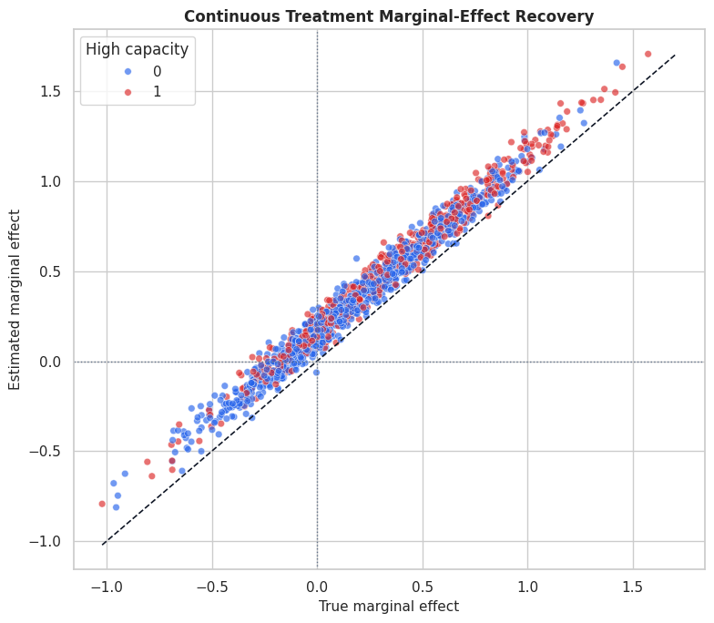
Continuous Marginal-Effect Recovery Plot

The next plot compares true and estimated marginal effects for held-out rows. The diagonal line is perfect recovery.

fig, ax = plt.subplots(figsize=(8, 7))
sns.scatterplot(
    data=continuous_eval,
    x="true_marginal_effect",
    y="estimated_marginal_effect",
    hue="high_capacity_segment",
    palette={0: "#2563eb", 1: "#dc2626"},
    alpha=0.65,
    s=30,
    ax=ax,
)
lims = [
    min(continuous_eval["true_marginal_effect"].min(), continuous_eval["estimated_marginal_effect"].min()),
    max(continuous_eval["true_marginal_effect"].max(), continuous_eval["estimated_marginal_effect"].max()),
]
ax.plot(lims, lims, color="#111827", linestyle="--", linewidth=1.2)
ax.axhline(0, color="#64748b", linestyle=":", linewidth=1)
ax.axvline(0, color="#64748b", linestyle=":", linewidth=1)
ax.set_title("Continuous Treatment Marginal-Effect Recovery")
ax.set_xlabel("True marginal effect")
ax.set_ylabel("Estimated marginal effect")
ax.legend(title="High capacity")
plt.tight_layout()
fig.savefig(FIGURE_DIR / "10_continuous_marginal_effect_recovery.png", dpi=160, bbox_inches="tight")
plt.show()

The scatterplot shows how well the estimated marginal effect tracks the true slope. Segment coloring helps reveal whether recovery differs across capacity groups.

Dose Contrast Sanity Check

Because the teaching outcome is linear in dose, the estimated effect from dose 0 to 2 should be about twice the estimated effect from dose 0 to 1. This cell checks that relationship directly.

dose_contrast_check = pd.DataFrame(
    {
        "metric": [
            "mean_estimated_effect_0_to_1",
            "mean_estimated_effect_0_to_2",
            "ratio_0_to_2_over_0_to_1",
            "mean_absolute_difference_between_2x_and_0_to_2",
        ],
        "value": [
            continuous_eval["estimated_effect_0_to_1"].mean(),
            continuous_eval["estimated_effect_0_to_2"].mean(),
            continuous_eval["estimated_effect_0_to_2"].mean() / continuous_eval["estimated_effect_0_to_1"].mean(),
            np.mean(np.abs(2 * continuous_eval["estimated_effect_0_to_1"] - continuous_eval["estimated_effect_0_to_2"])),
        ],
    }
)

dose_contrast_check.to_csv(TABLE_DIR / "10_continuous_dose_contrast_check.csv", index=False)
display(dose_contrast_check)

	metric	value
0	mean_estimated_effect_0_to_1	0.419174
1	mean_estimated_effect_0_to_2	0.838347
2	ratio_0_to_2_over_0_to_1	2.000000
3	mean_absolute_difference_between_2x_and_0_to_2	0.000000

The ratio and absolute difference confirm the expected linear-dose behavior. If the real causal question involved nonlinear saturation, we would need a treatment featurizer or a different dose-response strategy.

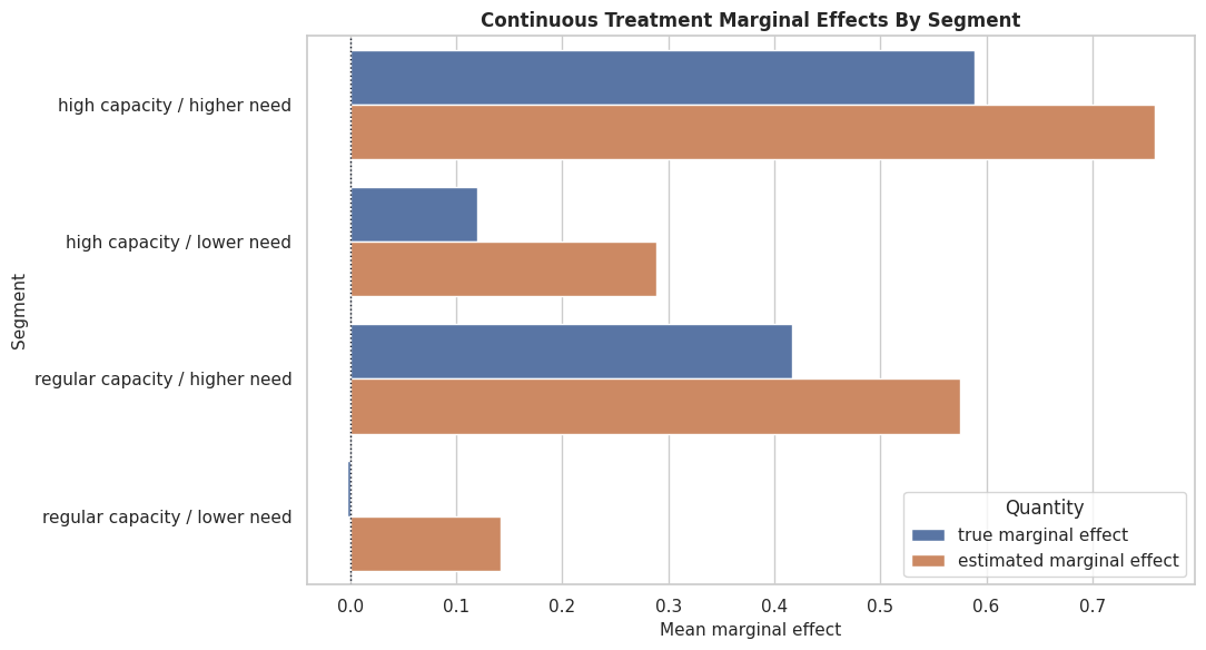
Segment-Level Continuous Effects

This cell summarizes estimated and true marginal effects by capacity and need segments. Segment summaries are often easier to communicate than row-level slopes.

continuous_segment_eval = continuous_eval.copy()
continuous_segment_eval["capacity_segment"] = np.where(continuous_segment_eval["high_capacity_segment"] == 1, "high capacity", "regular capacity")
continuous_segment_eval["need_segment"] = np.where(continuous_segment_eval["baseline_need"] > continuous_segment_eval["baseline_need"].median(), "higher need", "lower need")

continuous_segment_summary = (
    continuous_segment_eval.groupby(["capacity_segment", "need_segment"], observed=True)
    .agg(
        rows=("outcome", "size"),
        dose_mean=("treatment_intensity", "mean"),
        true_marginal_effect_mean=("true_marginal_effect", "mean"),
        estimated_marginal_effect_mean=("estimated_marginal_effect", "mean"),
        true_effect_0_to_2_mean=("true_effect_0_to_2", "mean"),
        estimated_effect_0_to_2_mean=("estimated_effect_0_to_2", "mean"),
        share_estimated_positive=("estimated_marginal_effect", lambda s: np.mean(s > 0)),
    )
    .reset_index()
)

continuous_segment_summary.to_csv(TABLE_DIR / "10_continuous_segment_summary.csv", index=False)
display(continuous_segment_summary)

	capacity_segment	need_segment	rows	dose_mean	true_marginal_effect_mean	estimated_marginal_effect_mean	true_effect_0_to_2_mean	estimated_effect_0_to_2_mean	share_estimated_positive
0	high capacity	higher need	244	1.666521	0.588862	0.758568	1.177724	1.517137	0.991803
1	high capacity	lower need	244	0.977828	0.119577	0.288660	0.239154	0.577319	0.799180
2	regular capacity	higher need	421	1.205265	0.417008	0.575637	0.834016	1.151274	0.957245
3	regular capacity	lower need	421	0.688809	-0.003173	0.141648	-0.006346	0.283296	0.665083

The segment table shows where increased treatment intensity appears most beneficial. It also exposes whether some segments have weaker estimated dose effects despite similar average dose levels.

Segment Continuous-Effect Plot

This plot compares true and estimated marginal effects by segment. It is a compact way to explain heterogeneous continuous-dose effects.

cont_segment_plot = continuous_segment_summary.copy()
cont_segment_plot["segment"] = cont_segment_plot["capacity_segment"] + " / " + cont_segment_plot["need_segment"]
cont_segment_long = cont_segment_plot.melt(
    id_vars="segment",
    value_vars=["true_marginal_effect_mean", "estimated_marginal_effect_mean"],
    var_name="quantity",
    value_name="marginal_effect",
)
cont_segment_long["quantity"] = cont_segment_long["quantity"].map(
    {
        "true_marginal_effect_mean": "true marginal effect",
        "estimated_marginal_effect_mean": "estimated marginal effect",
    }
)

fig, ax = plt.subplots(figsize=(11, 6))
sns.barplot(data=cont_segment_long, x="marginal_effect", y="segment", hue="quantity", ax=ax)
ax.axvline(0, color="#111827", linestyle=":", linewidth=1)
ax.set_title("Continuous Treatment Marginal Effects By Segment")
ax.set_xlabel("Mean marginal effect")
ax.set_ylabel("Segment")
ax.legend(title="Quantity")
plt.tight_layout()
fig.savefig(FIGURE_DIR / "10_continuous_segment_effects.png", dpi=160, bbox_inches="tight")
plt.show()

The segment plot shows whether the estimator preserves the broad ranking of groups. This is often more important for decision-making than perfect row-level recovery.

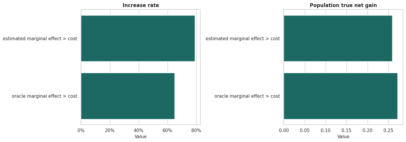
Dose-Increase Targeting Rule

A continuous-treatment model can support a policy such as “increase dose for rows whose estimated marginal effect is positive and high enough.” This cell compares a simple estimated rule to an oracle rule using the synthetic truth.

dose_increase_cost = 0.08
continuous_eval["estimated_increase_rule"] = (continuous_eval["estimated_marginal_effect"] > dose_increase_cost).astype(int)
continuous_eval["oracle_increase_rule"] = (continuous_eval["true_marginal_effect"] > dose_increase_cost).astype(int)

continuous_policy_summary = pd.DataFrame(
    [
        {
            "policy": "estimated marginal effect > cost",
            "increase_rate": continuous_eval["estimated_increase_rule"].mean(),
            "mean_true_net_gain_among_selected": (continuous_eval.loc[continuous_eval["estimated_increase_rule"] == 1, "true_marginal_effect"] - dose_increase_cost).mean(),
            "population_true_net_gain": ((continuous_eval["true_marginal_effect"] - dose_increase_cost) * continuous_eval["estimated_increase_rule"]).mean(),
            "share_selected_with_negative_net_truth": ((continuous_eval.loc[continuous_eval["estimated_increase_rule"] == 1, "true_marginal_effect"] - dose_increase_cost) < 0).mean(),
        },
        {
            "policy": "oracle marginal effect > cost",
            "increase_rate": continuous_eval["oracle_increase_rule"].mean(),
            "mean_true_net_gain_among_selected": (continuous_eval.loc[continuous_eval["oracle_increase_rule"] == 1, "true_marginal_effect"] - dose_increase_cost).mean(),
            "population_true_net_gain": ((continuous_eval["true_marginal_effect"] - dose_increase_cost) * continuous_eval["oracle_increase_rule"]).mean(),
            "share_selected_with_negative_net_truth": ((continuous_eval.loc[continuous_eval["oracle_increase_rule"] == 1, "true_marginal_effect"] - dose_increase_cost) < 0).mean(),
        },
    ]
)

continuous_policy_summary.to_csv(TABLE_DIR / "10_continuous_dose_increase_policy_summary.csv", index=False)
display(continuous_policy_summary)

	policy	increase_rate	mean_true_net_gain_among_selected	population_true_net_gain	share_selected_with_negative_net_truth
0	estimated marginal effect > cost	0.789474	0.328009	0.258955	0.178095
1	oracle marginal effect > cost	0.648872	0.418522	0.271567	0.000000

The estimated rule is a realistic version of dose targeting: it uses model-estimated marginal effects and a cost threshold. The oracle row shows the upper benchmark that would be available only if true effects were known.

Dose-Increase Policy Plot

The final policy plot compares increase rates and true net gains under the estimated and oracle dose-increase rules.

continuous_policy_plot = continuous_policy_summary.melt(
    id_vars="policy",
    value_vars=["increase_rate", "population_true_net_gain"],
    var_name="metric",
    value_name="value",
)
continuous_policy_plot["metric"] = continuous_policy_plot["metric"].map(
    {
        "increase_rate": "Increase rate",
        "population_true_net_gain": "Population true net gain",
    }
)

fig, axes = plt.subplots(1, 2, figsize=(14, 5))
for ax, metric in zip(axes, continuous_policy_plot["metric"].unique()):
    subset = continuous_policy_plot[continuous_policy_plot["metric"] == metric]
    sns.barplot(data=subset, x="value", y="policy", color="#0f766e", ax=ax)
    ax.set_title(metric)
    ax.set_xlabel("Value")
    ax.set_ylabel("")
    if metric == "Increase rate":
        ax.xaxis.set_major_formatter(PercentFormatter(1.0))
plt.tight_layout()
fig.savefig(FIGURE_DIR / "10_continuous_policy_comparison.png", dpi=160, bbox_inches="tight")
plt.show()

The policy plot translates marginal effects into a decision. Even in a continuous-dose setting, the model often becomes useful through a clear rule that says where to increase, decrease, or hold intensity.

Practical Checklist

The final checklist summarizes what to verify before using multiple-treatment or continuous-treatment estimates in a real analysis.

practical_checklist = pd.DataFrame(
    [
        {
            "topic": "Treatment definition",
            "multi_arm_question": "Are arms mutually exclusive and clearly named?",
            "continuous_question": "Is the dose numeric, ordered, and measured before the outcome window?",
        },
        {
            "topic": "Reference contrast",
            "multi_arm_question": "Which arm is the baseline for effect estimates?",
            "continuous_question": "Which finite dose contrast or marginal effect is being reported?",
        },
        {
            "topic": "Overlap and support",
            "multi_arm_question": "Does every arm have support in the covariate regions being compared?",
            "continuous_question": "Is there enough dose variation within important segments?",
        },
        {
            "topic": "Nuisance models",
            "multi_arm_question": "Can the arm assignment and outcome models learn useful signal?",
            "continuous_question": "Can the dose and outcome models learn useful signal?",
        },
        {
            "topic": "Decision rule",
            "multi_arm_question": "Will action use best-arm ranking, budget constraints, or arm-specific thresholds?",
            "continuous_question": "Will action use marginal-effect thresholds, dose caps, or cost-adjusted net effects?",
        },
        {
            "topic": "Reporting",
            "multi_arm_question": "Report arm-specific effects and the arm mix of the learned policy.",
            "continuous_question": "Report marginal effects, dose support, and the dose range where results apply.",
        },
    ]
)

practical_checklist.to_csv(TABLE_DIR / "10_multiple_and_continuous_treatment_checklist.csv", index=False)
display(practical_checklist)

	topic	multi_arm_question	continuous_question
0	Treatment definition	Are arms mutually exclusive and clearly named?	Is the dose numeric, ordered, and measured bef...
1	Reference contrast	Which arm is the baseline for effect estimates?	Which finite dose contrast or marginal effect ...
2	Overlap and support	Does every arm have support in the covariate r...	Is there enough dose variation within importan...
3	Nuisance models	Can the arm assignment and outcome models lear...	Can the dose and outcome models learn useful s...
4	Decision rule	Will action use best-arm ranking, budget const...	Will action use marginal-effect thresholds, do...
5	Reporting	Report arm-specific effects and the arm mix of...	Report marginal effects, dose support, and the...

The checklist keeps the final analysis grounded. Multiple treatments and continuous treatments are powerful, but they require careful contrast definitions and support diagnostics.

Summary

This notebook extended the EconML tutorial sequence beyond binary treatments.

The multi-arm section showed how to:

• define a baseline arm and active-arm contrasts;
• estimate arm-specific CATEs with DRLearner;
• compare active arms for the same row;
• convert arm effects into an estimated best-arm policy;
• evaluate arm-specific recovery and policy regret on synthetic truth.

The continuous-treatment section showed how to:

• define marginal effects and finite dose contrasts;
• inspect dose support before modeling;
• estimate heterogeneous dose slopes with LinearDML;
• compare estimated slopes with known synthetic truth;
• turn marginal effects into a dose-increase rule.

The next tutorial introduces instrumental-variable estimators, which are useful when treatment is confounded by unobserved factors but a credible instrument is available.