EconML Tutorial 03: LinearDML And SparseLinearDML

This notebook focuses on two closely related EconML estimators:

• LinearDML, which estimates a linear CATE model over chosen effect modifiers;
• SparseLinearDML, which is designed for wider effect-modifier spaces where only some features are expected to matter.

The teaching question is:

Which pre-treatment features appear to change the size of the treatment effect, and can we estimate those effect drivers after adjusting for confounding?

This is the first estimator-specific notebook in the EconML tutorial sequence. The previous notebook built DML from scratch. Here we lean into the library API and focus on practical modeling decisions: feature roles, coefficient reading, sparse selection behavior, CATE recovery, and treatment targeting.

Learning Goals

By the end of this notebook, you should be able to:

• fit LinearDML with observed confounders and effect modifiers;
• fit SparseLinearDML on a wider set of candidate effect modifiers;
• explain the difference between nuisance models and the final CATE model;
• read final-stage CATE coefficients without confusing them for outcome-model coefficients;
• compare dense and sparse CATE estimates against known truth in a simulation;
• diagnose coefficient stability, noise-feature shrinkage, CATE ranking quality, and segment-level recovery;
• decide when a linear CATE model is a reasonable first estimator.

Why LinearDML Comes First

LinearDML is often the easiest serious EconML estimator to explain. It combines two useful properties:

• flexible nuisance models can estimate the baseline outcome and treatment assignment process;
• the final treatment-effect model remains linear and readable.

That means the model can adjust for confounding with machine learning while still producing coefficient-style CATE drivers. For example, a positive coefficient on baseline_need means the estimated treatment effect is larger for higher values of baseline_need, after the DML adjustment process.

SparseLinearDML keeps the same broad structure but adds sparse regularization in the final CATE stage. That is useful when we have many possible effect modifiers and want the final model to concentrate on the strongest signals.

LinearDML Versus SparseLinearDML

The next table summarizes how to think about the two estimators before writing code.

from pathlib import Path
import os
import warnings
import importlib.metadata as importlib_metadata

# Keep Matplotlib cache files in a writable location during notebook execution.
os.environ.setdefault("MPLCONFIGDIR", "/tmp/matplotlib-ranking-sys")

warnings.filterwarnings("default")
warnings.filterwarnings("ignore", category=DeprecationWarning)
warnings.filterwarnings("ignore", category=PendingDeprecationWarning)
warnings.filterwarnings("ignore", category=FutureWarning)
warnings.filterwarnings("ignore", message=".*IProgress not found.*")
warnings.filterwarnings("ignore", message=".*X does not have valid feature names.*")
warnings.filterwarnings("ignore", message=".*The final model has a nonzero intercept.*")
warnings.filterwarnings("ignore", message=".*Co-variance matrix is underdetermined.*")
warnings.filterwarnings("ignore", module="sklearn.linear_model._logistic")

import numpy as np
import pandas as pd
import matplotlib.pyplot as plt
import seaborn as sns

from IPython.display import display
from sklearn.ensemble import RandomForestClassifier, RandomForestRegressor
from sklearn.metrics import brier_score_loss, log_loss, mean_squared_error, roc_auc_score
from sklearn.model_selection import KFold, StratifiedKFold, cross_val_predict, train_test_split

try:
    import econml
    from econml.dml import LinearDML, SparseLinearDML
    ECONML_AVAILABLE = True
    ECONML_VERSION = getattr(econml, "__version__", "unknown")
except Exception as exc:
    ECONML_AVAILABLE = False
    ECONML_VERSION = f"import failed: {type(exc).__name__}: {exc}"

RANDOM_SEED = 2026
rng = np.random.default_rng(RANDOM_SEED)

OUTPUT_DIR = Path("outputs")
FIGURE_DIR = OUTPUT_DIR / "figures"
TABLE_DIR = OUTPUT_DIR / "tables"
FIGURE_DIR.mkdir(parents=True, exist_ok=True)
TABLE_DIR.mkdir(parents=True, exist_ok=True)

sns.set_theme(style="whitegrid", context="notebook")
pd.set_option("display.max_columns", 140)
pd.set_option("display.float_format", lambda value: f"{value:,.4f}")

estimator_map = pd.DataFrame(
    [
        {
            "estimator": "LinearDML",
            "final CATE model": "Dense linear model over X",
            "best first use": "A moderate number of meaningful effect modifiers",
            "main strength": "Readable coefficient-style effect drivers",
            "main risk": "Can assign visible coefficients to weak or noisy modifiers",
        },
        {
            "estimator": "SparseLinearDML",
            "final CATE model": "Sparse regularized linear model over X",
            "best first use": "A wider candidate feature set with only some true effect drivers",
            "main strength": "Shrinks weak CATE drivers and can highlight a smaller feature set",
            "main risk": "Regularization can shrink real but subtle signals too much",
        },
    ]
)

estimator_map.to_csv(TABLE_DIR / "03_estimator_map.csv", index=False)
print(f"EconML available: {ECONML_AVAILABLE}")
print(f"EconML version: {ECONML_VERSION}")
print(f"Figures will be saved to: {FIGURE_DIR.resolve()}")
print(f"Tables will be saved to: {TABLE_DIR.resolve()}")
display(estimator_map)

EconML available: True
EconML version: 0.16.0
Figures will be saved to: /home/apex/Documents/ranking_sys/notebooks/tutorials/econml/outputs/figures
Tables will be saved to: /home/apex/Documents/ranking_sys/notebooks/tutorials/econml/outputs/tables

	estimator	final CATE model	best first use	main strength	main risk
0	LinearDML	Dense linear model over X	A moderate number of meaningful effect modifiers	Readable coefficient-style effect drivers	Can assign visible coefficients to weak or noi...
1	SparseLinearDML	Sparse regularized linear model over X	A wider candidate feature set with only some t...	Shrinks weak CATE drivers and can highlight a ...	Regularization can shrink real but subtle sign...

What this shows: both estimators use DML, but they differ in the final CATE stage. The nuisance models handle adjustment; the final stage decides how treatment-effect heterogeneity is represented.

Data-Generating Design

The synthetic dataset below is designed to teach a specific modeling problem:

• treatment is confounded by observed pre-treatment features;
• the outcome has a flexible baseline component;
• the true treatment effect is sparse and linear in a subset of candidate effect modifiers;
• several noise features are included as tempting but irrelevant effect modifiers.

This gives LinearDML and SparseLinearDML something meaningful to compare. A dense linear model can estimate every candidate coefficient, while a sparse model should concentrate more of the final-stage weight on the real effect drivers.

n = 3_200

baseline_need = rng.normal(0, 1, size=n)
prior_engagement = rng.normal(0, 1, size=n)
friction_score = 0.55 * baseline_need - 0.25 * prior_engagement + rng.normal(0, 0.85, size=n)
price_sensitivity = rng.normal(0, 1, size=n)
trust_score = rng.normal(0, 1, size=n)
content_affinity = 0.35 * prior_engagement + rng.normal(0, 0.95, size=n)
recency_gap = rng.normal(0, 1, size=n)
region_risk = rng.binomial(1, 0.34, size=n)
high_need_segment = (baseline_need > 0.55).astype(int)

account_tenure = rng.normal(0, 1, size=n)
seasonality_index = rng.normal(0, 1, size=n)
device_stability = rng.normal(0, 1, size=n)

noise_features = {
    f"noise_modifier_{i:02d}": rng.normal(0, 1, size=n)
    for i in range(1, 13)
}

propensity_logit = (
    -0.15
    + 0.75 * baseline_need
    + 0.45 * prior_engagement
    + 0.35 * friction_score
    + 0.30 * content_affinity
    - 0.25 * trust_score
    + 0.25 * region_risk
    + 0.20 * high_need_segment
    - 0.35 * account_tenure
    + 0.25 * seasonality_index
    + 0.20 * noise_features["noise_modifier_01"]
)
propensity = 1 / (1 + np.exp(-propensity_logit))
propensity = np.clip(propensity, 0.03, 0.97)
treatment = rng.binomial(1, propensity, size=n)

true_cate = (
    0.42
    + 0.30 * baseline_need
    + 0.22 * prior_engagement
    - 0.24 * friction_score
    - 0.18 * price_sensitivity
    + 0.16 * content_affinity
    - 0.12 * region_risk
    + 0.24 * high_need_segment
)

baseline_outcome = (
    2.20
    + 0.80 * baseline_need
    + 0.55 * prior_engagement
    - 0.50 * friction_score
    + 0.30 * trust_score
    + 0.35 * account_tenure
    + 0.25 * seasonality_index
    + 0.20 * device_stability
    + 0.18 * region_risk
    + 0.12 * baseline_need * friction_score
    - 0.10 * price_sensitivity * trust_score
)
noise = rng.normal(0, 0.90, size=n)
outcome = baseline_outcome + true_cate * treatment + noise

teaching_df = pd.DataFrame(
    {
        "user_id": np.arange(n),
        "baseline_need": baseline_need,
        "prior_engagement": prior_engagement,
        "friction_score": friction_score,
        "price_sensitivity": price_sensitivity,
        "trust_score": trust_score,
        "content_affinity": content_affinity,
        "recency_gap": recency_gap,
        "region_risk": region_risk,
        "high_need_segment": high_need_segment,
        "account_tenure": account_tenure,
        "seasonality_index": seasonality_index,
        "device_stability": device_stability,
        **noise_features,
        "propensity": propensity,
        "treatment": treatment,
        "outcome": outcome,
        "true_cate": true_cate,
        "baseline_outcome_mean": baseline_outcome,
    }
)

teaching_df.head()

	user_id	baseline_need	prior_engagement	friction_score	price_sensitivity	trust_score	content_affinity	recency_gap	region_risk	high_need_segment	account_tenure	seasonality_index	device_stability	noise_modifier_01	noise_modifier_02	noise_modifier_03	noise_modifier_04	noise_modifier_05	noise_modifier_06	noise_modifier_07	noise_modifier_08	noise_modifier_09	noise_modifier_10	noise_modifier_11	noise_modifier_12	propensity	treatment	outcome	true_cate	baseline_outcome_mean
0	0	-0.7931	-1.2901	-0.3725	0.3794	-1.1530	-1.7022	-0.7477	1	0	-3.0473	-0.3020	-0.9402	2.2139	3.3326	1.0087	-0.0561	0.3949	0.2200	-0.2702	0.4688	1.5857	0.6316	0.5724	0.0884	0.5014	0	-0.3295	-0.4730	-0.3746
1	1	0.2406	0.2599	-0.4635	0.2294	-0.9692	1.3488	-0.4711	0	0	-0.5008	-0.4229	1.2210	0.6131	-0.6644	-1.3256	1.2507	0.0068	-1.3397	0.8011	-0.6055	0.2176	-0.8961	-1.7315	-0.4224	0.6951	1	4.1711	0.8351	2.4484
2	2	-1.8963	-0.3197	-0.9924	-0.0940	-1.2255	-0.5499	0.0474	0	0	-0.0048	-0.8700	-1.7494	-0.0209	-0.1113	-1.2531	-0.7628	-0.7286	0.1870	-0.2217	-0.6922	0.9850	-0.3564	1.8125	0.7178	0.1051	0	0.9768	-0.0521	0.2809
3	3	1.3958	-0.2729	0.3750	0.5754	0.6809	-1.5469	1.4382	0	1	1.0852	-0.2230	-2.3089	0.9227	-0.0710	-1.1789	-1.0234	-1.0542	1.8849	-0.0726	-0.6707	-0.7611	-0.5606	0.2016	-1.8027	0.5548	0	5.7941	0.5776	3.0692
4	4	0.6383	-1.4263	0.6936	-1.5145	0.5773	0.6027	2.8067	0	1	-1.8344	-0.9164	-0.2073	-0.3209	-0.6215	-0.9096	-0.5394	-0.7578	0.0065	0.2065	1.3599	0.1552	-0.9609	1.6112	-0.3389	0.6260	0	3.0364	0.7403	0.9805

What this shows: the table has both real modeling fields and oracle fields. In the model-fitting steps we will use only pre-treatment observed features, treatment, and outcome. true_cate, propensity, and baseline_outcome_mean are kept only for teaching checks.

Field Dictionary

A field dictionary is especially useful in estimator tutorials because it separates three ideas that are easy to mix up:

• features used to explain treatment-effect heterogeneity;
• controls used to remove confounding;
• oracle fields available only because this is a simulation.

signal_modifier_cols = [
    "baseline_need",
    "prior_engagement",
    "friction_score",
    "price_sensitivity",
    "content_affinity",
    "region_risk",
    "high_need_segment",
]
weak_or_null_modifier_cols = ["trust_score", "recency_gap"] + list(noise_features.keys())
effect_modifier_cols = signal_modifier_cols + weak_or_null_modifier_cols
control_cols = ["account_tenure", "seasonality_index", "device_stability"]
all_observed_covariates = effect_modifier_cols + control_cols

field_rows = []
for col in effect_modifier_cols:
    field_rows.append(
        {
            "column": col,
            "model_role": "X candidate effect modifier",
            "observed_in_real_analysis": "yes",
            "description": "Pre-treatment feature allowed to modify the treatment effect.",
            "true_cate_driver": "yes" if col in signal_modifier_cols else "no",
        }
    )
for col in control_cols:
    field_rows.append(
        {
            "column": col,
            "model_role": "W control",
            "observed_in_real_analysis": "yes",
            "description": "Pre-treatment feature used for adjustment but not used for CATE reporting.",
            "true_cate_driver": "no",
        }
    )
for col, role, description in [
    ("treatment", "treatment", "Binary intervention indicator."),
    ("outcome", "outcome", "Observed post-treatment outcome."),
    ("propensity", "oracle", "True treatment probability from the simulated assignment process."),
    ("true_cate", "oracle", "Known individual treatment effect used for tutorial grading."),
    ("baseline_outcome_mean", "oracle", "Mean untreated outcome component before random noise."),
]:
    field_rows.append(
        {
            "column": col,
            "model_role": role,
            "observed_in_real_analysis": "yes" if role in ["treatment", "outcome"] else "no",
            "description": description,
            "true_cate_driver": "not applicable",
        }
    )

field_dictionary = pd.DataFrame(field_rows)
field_dictionary.to_csv(TABLE_DIR / "03_field_dictionary.csv", index=False)
display(field_dictionary.head(30))

	column	model_role	observed_in_real_analysis	description	true_cate_driver
0	baseline_need	X candidate effect modifier	yes	Pre-treatment feature allowed to modify the tr...	yes
1	prior_engagement	X candidate effect modifier	yes	Pre-treatment feature allowed to modify the tr...	yes
2	friction_score	X candidate effect modifier	yes	Pre-treatment feature allowed to modify the tr...	yes
3	price_sensitivity	X candidate effect modifier	yes	Pre-treatment feature allowed to modify the tr...	yes
4	content_affinity	X candidate effect modifier	yes	Pre-treatment feature allowed to modify the tr...	yes
5	region_risk	X candidate effect modifier	yes	Pre-treatment feature allowed to modify the tr...	yes
6	high_need_segment	X candidate effect modifier	yes	Pre-treatment feature allowed to modify the tr...	yes
7	trust_score	X candidate effect modifier	yes	Pre-treatment feature allowed to modify the tr...	no
8	recency_gap	X candidate effect modifier	yes	Pre-treatment feature allowed to modify the tr...	no
9	noise_modifier_01	X candidate effect modifier	yes	Pre-treatment feature allowed to modify the tr...	no
10	noise_modifier_02	X candidate effect modifier	yes	Pre-treatment feature allowed to modify the tr...	no
11	noise_modifier_03	X candidate effect modifier	yes	Pre-treatment feature allowed to modify the tr...	no
12	noise_modifier_04	X candidate effect modifier	yes	Pre-treatment feature allowed to modify the tr...	no
13	noise_modifier_05	X candidate effect modifier	yes	Pre-treatment feature allowed to modify the tr...	no
14	noise_modifier_06	X candidate effect modifier	yes	Pre-treatment feature allowed to modify the tr...	no
15	noise_modifier_07	X candidate effect modifier	yes	Pre-treatment feature allowed to modify the tr...	no
16	noise_modifier_08	X candidate effect modifier	yes	Pre-treatment feature allowed to modify the tr...	no
17	noise_modifier_09	X candidate effect modifier	yes	Pre-treatment feature allowed to modify the tr...	no
18	noise_modifier_10	X candidate effect modifier	yes	Pre-treatment feature allowed to modify the tr...	no
19	noise_modifier_11	X candidate effect modifier	yes	Pre-treatment feature allowed to modify the tr...	no
20	noise_modifier_12	X candidate effect modifier	yes	Pre-treatment feature allowed to modify the tr...	no
21	account_tenure	W control	yes	Pre-treatment feature used for adjustment but ...	no
22	seasonality_index	W control	yes	Pre-treatment feature used for adjustment but ...	no
23	device_stability	W control	yes	Pre-treatment feature used for adjustment but ...	no
24	treatment	treatment	yes	Binary intervention indicator.	not applicable
25	outcome	outcome	yes	Observed post-treatment outcome.	not applicable
26	propensity	oracle	no	True treatment probability from the simulated ...	not applicable
27	true_cate	oracle	no	Known individual treatment effect used for tut...	not applicable
28	baseline_outcome_mean	oracle	no	Mean untreated outcome component before random...	not applicable

What this shows: some X columns are true CATE drivers and others are deliberately irrelevant. That is the point of this lesson: wide candidate effect-modifier sets are common, and sparse final-stage models can help control clutter.

True CATE Equation

Since this is a simulation, we can show the real treatment-effect equation. The true CATE is sparse: only seven candidate effect modifiers have nonzero coefficients.

In real work, this table does not exist. We would use domain logic, robustness checks, and validation strategies rather than ground truth.

true_coefficient_map = {
    "cate_intercept": 0.42,
    "baseline_need": 0.30,
    "prior_engagement": 0.22,
    "friction_score": -0.24,
    "price_sensitivity": -0.18,
    "content_affinity": 0.16,
    "region_risk": -0.12,
    "high_need_segment": 0.24,
}

true_coef_table = pd.DataFrame(
    [{"term": "cate_intercept", "true_cate_coefficient": true_coefficient_map["cate_intercept"], "is_true_driver": True}]
    + [
        {
            "term": col,
            "true_cate_coefficient": true_coefficient_map.get(col, 0.0),
            "is_true_driver": col in true_coefficient_map,
        }
        for col in effect_modifier_cols
    ]
)

true_coef_table.to_csv(TABLE_DIR / "03_true_cate_coefficients.csv", index=False)
display(true_coef_table)

	term	true_cate_coefficient	is_true_driver
0	cate_intercept	0.4200	True
1	baseline_need	0.3000	True
2	prior_engagement	0.2200	True
3	friction_score	-0.2400	True
4	price_sensitivity	-0.1800	True
5	content_affinity	0.1600	True
6	region_risk	-0.1200	True
7	high_need_segment	0.2400	True
8	trust_score	0.0000	False
9	recency_gap	0.0000	False
10	noise_modifier_01	0.0000	False
11	noise_modifier_02	0.0000	False
12	noise_modifier_03	0.0000	False
13	noise_modifier_04	0.0000	False
14	noise_modifier_05	0.0000	False
15	noise_modifier_06	0.0000	False
16	noise_modifier_07	0.0000	False
17	noise_modifier_08	0.0000	False
18	noise_modifier_09	0.0000	False
19	noise_modifier_10	0.0000	False
20	noise_modifier_11	0.0000	False
21	noise_modifier_12	0.0000	False

What this shows: LinearDML and SparseLinearDML are being asked to estimate this treatment-effect pattern from observational data. The nuisance models must remove confounding first; the final CATE model then tries to recover these coefficients.

Basic Shape And True Effects

Before fitting anything, we summarize the sample size, treatment rate, outcome level, and true effect distribution. This establishes the scale of the problem.

basic_summary = pd.DataFrame(
    [
        {"metric": "rows", "value": len(teaching_df)},
        {"metric": "columns", "value": teaching_df.shape[1]},
        {"metric": "candidate_X_features", "value": len(effect_modifier_cols)},
        {"metric": "W_controls", "value": len(control_cols)},
        {"metric": "treatment_rate", "value": teaching_df["treatment"].mean()},
        {"metric": "outcome_mean", "value": teaching_df["outcome"].mean()},
        {"metric": "true_ate", "value": teaching_df["true_cate"].mean()},
        {"metric": "true_cate_std", "value": teaching_df["true_cate"].std()},
        {"metric": "true_cate_min", "value": teaching_df["true_cate"].min()},
        {"metric": "true_cate_max", "value": teaching_df["true_cate"].max()},
    ]
)

basic_summary.to_csv(TABLE_DIR / "03_basic_summary.csv", index=False)
display(basic_summary)

	metric	value
0	rows	3,200.0000
1	columns	30.0000
2	candidate_X_features	21.0000
3	W_controls	3.0000
4	treatment_rate	0.4875
5	outcome_mean	2.6234
6	true_ate	0.4614
7	true_cate_std	0.5193
8	true_cate_min	-1.4146
9	true_cate_max	2.0582

What this shows: the tutorial has enough rows for cross-fitting and enough candidate modifiers to make sparse modeling relevant. The true CATE standard deviation confirms that there is meaningful heterogeneity to estimate.

Raw Treated-Versus-Control Difference

A raw difference in observed outcomes is not a DML estimate. It ignores the treatment assignment process and will usually be biased when treatment is confounded.

The next cell compares the raw outcome difference with the true ATE.

raw_group_summary = (
    teaching_df.groupby("treatment")
    .agg(
        rows=("outcome", "size"),
        observed_outcome_mean=("outcome", "mean"),
        true_cate_mean=("true_cate", "mean"),
        propensity_mean=("propensity", "mean"),
        baseline_need_mean=("baseline_need", "mean"),
        prior_engagement_mean=("prior_engagement", "mean"),
        friction_score_mean=("friction_score", "mean"),
    )
    .reset_index()
)

raw_difference = (
    raw_group_summary.loc[raw_group_summary["treatment"].eq(1), "observed_outcome_mean"].iloc[0]
    - raw_group_summary.loc[raw_group_summary["treatment"].eq(0), "observed_outcome_mean"].iloc[0]
)
true_ate = teaching_df["true_cate"].mean()

raw_difference_summary = pd.DataFrame(
    [
        {"quantity": "raw treated minus untreated outcome mean", "value": raw_difference},
        {"quantity": "true ATE", "value": true_ate},
        {"quantity": "raw difference minus true ATE", "value": raw_difference - true_ate},
    ]
)

raw_group_summary.to_csv(TABLE_DIR / "03_raw_group_summary.csv", index=False)
raw_difference_summary.to_csv(TABLE_DIR / "03_raw_difference_vs_truth.csv", index=False)
display(raw_group_summary)
display(raw_difference_summary)

	treatment	rows	observed_outcome_mean	true_cate_mean	propensity_mean	baseline_need_mean	prior_engagement_mean	friction_score_mean
0	0	1640	2.1097	0.3294	0.3731	-0.4104	-0.1270	-0.2990
1	1	1560	3.1635	0.6001	0.6226	0.3651	0.1963	0.2438

	quantity	value
0	raw treated minus untreated outcome mean	1.0538
1	true ATE	0.4614
2	raw difference minus true ATE	0.5924

What this shows: treated rows have different baseline covariate profiles and different average true CATE. This is why the estimator needs both nuisance adjustment and a treatment-effect model.

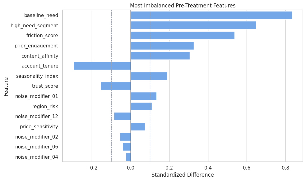
Covariate Balance Table

The standardized mean difference measures how different treated and untreated groups are before adjustment. Large values are a sign that treatment assignment is strongly related to covariates.

balance_rows = []
for col in all_observed_covariates:
    treated_values = teaching_df.loc[teaching_df["treatment"].eq(1), col]
    control_values = teaching_df.loc[teaching_df["treatment"].eq(0), col]
    pooled_sd = np.sqrt((treated_values.var(ddof=1) + control_values.var(ddof=1)) / 2)
    balance_rows.append(
        {
            "covariate": col,
            "treated_mean": treated_values.mean(),
            "control_mean": control_values.mean(),
            "standardized_difference": (treated_values.mean() - control_values.mean()) / pooled_sd,
        }
    )

balance_table = pd.DataFrame(balance_rows).sort_values("standardized_difference", key=lambda s: s.abs(), ascending=False)
balance_table.to_csv(TABLE_DIR / "03_covariate_balance.csv", index=False)
display(balance_table.head(15))

	covariate	treated_mean	control_mean	standardized_difference
0	baseline_need	0.3651	-0.4104	0.8335
6	high_need_segment	0.4314	0.1506	0.6498
2	friction_score	0.2438	-0.2990	0.5359
1	prior_engagement	0.1963	-0.1270	0.3255
4	content_affinity	0.1886	-0.1187	0.3058
21	account_tenure	-0.1545	0.1409	-0.2953
22	seasonality_index	0.0763	-0.1104	0.1904
7	trust_score	-0.0866	0.0670	-0.1548
9	noise_modifier_01	0.0614	-0.0690	0.1331
5	region_risk	0.3474	0.2963	0.1095
20	noise_modifier_12	-0.0617	0.0256	-0.0870
3	price_sensitivity	0.0341	-0.0396	0.0737
10	noise_modifier_02	-0.0451	0.0120	-0.0567
14	noise_modifier_06	-0.0386	0.0033	-0.0418
12	noise_modifier_04	-0.0085	0.0178	-0.0258

What this shows: the top imbalance features are exactly the kind of variables that nuisance models need to account for. DML does not erase the need for careful adjustment design; it operationalizes that design with cross-fitted prediction models.

Covariate Balance Plot

The plot below focuses on the most imbalanced features so the confounding pattern is easy to scan.

plot_balance = balance_table.head(15).copy()
fig, ax = plt.subplots(figsize=(10, 6))
sns.barplot(
    data=plot_balance,
    x="standardized_difference",
    y="covariate",
    color="#60a5fa",
    ax=ax,
)
ax.axvline(0, color="#111827", linewidth=1)
ax.axvline(0.10, color="#9ca3af", linewidth=1, linestyle="--")
ax.axvline(-0.10, color="#9ca3af", linewidth=1, linestyle="--")
ax.set_title("Most Imbalanced Pre-Treatment Features")
ax.set_xlabel("Standardized Difference")
ax.set_ylabel("Feature")
plt.tight_layout()
fig.savefig(FIGURE_DIR / "03_covariate_balance.png", dpi=160, bbox_inches="tight")
plt.show()

What this shows: the treatment group is systematically different before treatment. The DML estimators should be judged against this context, not against a fictional randomized design.

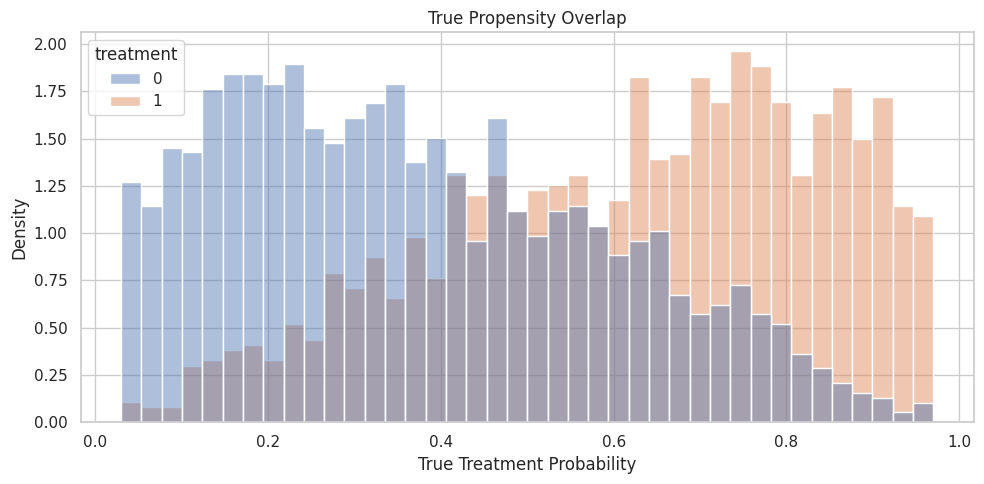
Propensity Overlap

Overlap checks whether treated and untreated rows exist across similar treatment-probability regions. Weak overlap makes treatment-effect estimation more extrapolative.

We know the true propensity in this simulation. In real data, we would estimate it.

propensity_summary = (
    teaching_df.assign(propensity_bucket=pd.cut(teaching_df["propensity"], bins=np.linspace(0, 1, 11), include_lowest=True))
    .groupby("propensity_bucket", observed=True)
    .agg(rows=("propensity", "size"), treatment_rate=("treatment", "mean"), true_cate_mean=("true_cate", "mean"))
    .reset_index()
)
propensity_summary["propensity_bucket"] = propensity_summary["propensity_bucket"].astype(str)
propensity_summary.to_csv(TABLE_DIR / "03_propensity_bucket_summary.csv", index=False)
display(propensity_summary)

	propensity_bucket	rows	treatment_rate	true_cate_mean
0	(-0.001, 0.1]	157	0.0637	-0.0866
1	(0.1, 0.2]	333	0.1622	0.0843
2	(0.2, 0.3]	350	0.2343	0.2584
3	(0.3, 0.4]	412	0.3325	0.2985
4	(0.4, 0.5]	386	0.4715	0.3945
5	(0.5, 0.6]	358	0.5140	0.5080
6	(0.6, 0.7]	378	0.6323	0.5834
7	(0.7, 0.8]	377	0.7454	0.7045
8	(0.8, 0.9]	293	0.8396	0.9102
9	(0.9, 1.0]	156	0.9295	1.0357

What this shows: most propensity buckets contain observed data, which is good for teaching. The treatment rate rises with the propensity bucket, confirming that the assignment mechanism is not random.

Propensity Overlap Plot

The histogram gives a visual check of how much treated and untreated rows overlap in propensity space.

fig, ax = plt.subplots(figsize=(10, 5))
sns.histplot(
    data=teaching_df,
    x="propensity",
    hue="treatment",
    bins=40,
    stat="density",
    common_norm=False,
    alpha=0.45,
    ax=ax,
)
ax.set_title("True Propensity Overlap")
ax.set_xlabel("True Treatment Probability")
ax.set_ylabel("Density")
plt.tight_layout()
fig.savefig(FIGURE_DIR / "03_propensity_overlap.png", dpi=160, bbox_inches="tight")
plt.show()

What this shows: overlap is imperfect but usable. That is a realistic teaching setting for DML: enough support to estimate effects, but enough confounding that naive comparisons are misleading.

X And W Roles

For these estimators:

• X is the feature set used in the final CATE model;
• W is the control set used for adjustment in nuisance models.

The same observed feature can sometimes be defensibly placed in either set. The key question is whether you want the reported treatment effect to vary along that feature.

role_table = pd.DataFrame(
    [
        {
            "feature": col,
            "econml_role": "X",
            "true_cate_driver": col in signal_modifier_cols,
            "reason": "Candidate effect modifier used by the final CATE model.",
        }
        for col in effect_modifier_cols
    ]
    + [
        {
            "feature": col,
            "econml_role": "W",
            "true_cate_driver": False,
            "reason": "Adjustment control used by nuisance models, not by the final CATE model.",
        }
        for col in control_cols
    ]
)

role_table.to_csv(TABLE_DIR / "03_x_w_role_table.csv", index=False)
display(role_table)

	feature	econml_role	true_cate_driver	reason
0	baseline_need	X	True	Candidate effect modifier used by the final CA...
1	prior_engagement	X	True	Candidate effect modifier used by the final CA...
2	friction_score	X	True	Candidate effect modifier used by the final CA...
3	price_sensitivity	X	True	Candidate effect modifier used by the final CA...
4	content_affinity	X	True	Candidate effect modifier used by the final CA...
5	region_risk	X	True	Candidate effect modifier used by the final CA...
6	high_need_segment	X	True	Candidate effect modifier used by the final CA...
7	trust_score	X	False	Candidate effect modifier used by the final CA...
8	recency_gap	X	False	Candidate effect modifier used by the final CA...
9	noise_modifier_01	X	False	Candidate effect modifier used by the final CA...
10	noise_modifier_02	X	False	Candidate effect modifier used by the final CA...
11	noise_modifier_03	X	False	Candidate effect modifier used by the final CA...
12	noise_modifier_04	X	False	Candidate effect modifier used by the final CA...
13	noise_modifier_05	X	False	Candidate effect modifier used by the final CA...
14	noise_modifier_06	X	False	Candidate effect modifier used by the final CA...
15	noise_modifier_07	X	False	Candidate effect modifier used by the final CA...
16	noise_modifier_08	X	False	Candidate effect modifier used by the final CA...
17	noise_modifier_09	X	False	Candidate effect modifier used by the final CA...
18	noise_modifier_10	X	False	Candidate effect modifier used by the final CA...
19	noise_modifier_11	X	False	Candidate effect modifier used by the final CA...
20	noise_modifier_12	X	False	Candidate effect modifier used by the final CA...
21	account_tenure	W	False	Adjustment control used by nuisance models, no...
22	seasonality_index	W	False	Adjustment control used by nuisance models, no...
23	device_stability	W	False	Adjustment control used by nuisance models, no...

What this shows: SparseLinearDML does not decide which variables are pre-treatment or causally admissible. It only regularizes among the X features we provide. The analyst still has to define a valid feature set.

Train And Test Split

The train set is used to fit nuisance models and CATE estimators. The test set is reserved for truth-known evaluation of CATE accuracy and ranking behavior.

train_idx, test_idx = train_test_split(
    teaching_df.index,
    test_size=0.35,
    random_state=RANDOM_SEED,
    stratify=teaching_df["treatment"],
)

train_df = teaching_df.loc[train_idx].reset_index(drop=True)
test_df = teaching_df.loc[test_idx].reset_index(drop=True)

split_summary = pd.DataFrame(
    [
        {"split": "train", "rows": len(train_df), "treatment_rate": train_df["treatment"].mean(), "true_ate": train_df["true_cate"].mean()},
        {"split": "test", "rows": len(test_df), "treatment_rate": test_df["treatment"].mean(), "true_ate": test_df["true_cate"].mean()},
    ]
)

split_summary.to_csv(TABLE_DIR / "03_train_test_split_summary.csv", index=False)
display(split_summary)

	split	rows	treatment_rate	true_ate
0	train	2080	0.4875	0.4522
1	test	1120	0.4875	0.4783

What this shows: the split preserves treatment balance and keeps the true ATE similar across train and test. That makes estimator comparisons easier to read.

Modeling Matrices

This cell prepares the arrays and data frames used by EconML. The most important modeling constraint is that oracle fields never enter X, W, or nuisance features.

Y_train = train_df["outcome"].to_numpy()
T_train = train_df["treatment"].to_numpy()
Y_test = test_df["outcome"].to_numpy()
T_test = test_df["treatment"].to_numpy()

X_train = train_df[effect_modifier_cols]
X_test = test_df[effect_modifier_cols]
W_train = train_df[control_cols]
W_test = test_df[control_cols]

nuisance_train = train_df[all_observed_covariates]
nuisance_test = test_df[all_observed_covariates]
true_cate_train = train_df["true_cate"].to_numpy()
true_cate_test = test_df["true_cate"].to_numpy()

matrix_summary = pd.DataFrame(
    [
        {"object": "Y_train", "rows": Y_train.shape[0], "columns": 1, "meaning": "Observed outcome."},
        {"object": "T_train", "rows": T_train.shape[0], "columns": 1, "meaning": "Observed binary treatment."},
        {"object": "X_train", "rows": X_train.shape[0], "columns": X_train.shape[1], "meaning": "Candidate effect modifiers."},
        {"object": "W_train", "rows": W_train.shape[0], "columns": W_train.shape[1], "meaning": "Controls for adjustment."},
        {"object": "nuisance_train", "rows": nuisance_train.shape[0], "columns": nuisance_train.shape[1], "meaning": "Observed pre-treatment features for separate nuisance diagnostics."},
    ]
)

matrix_summary.to_csv(TABLE_DIR / "03_model_matrix_summary.csv", index=False)
display(matrix_summary)

	object	rows	columns	meaning
0	Y_train	2080	1	Observed outcome.
1	T_train	2080	1	Observed binary treatment.
2	X_train	2080	21	Candidate effect modifiers.
3	W_train	2080	3	Controls for adjustment.
4	nuisance_train	2080	24	Observed pre-treatment features for separate n...

What this shows: X is intentionally wider than the true CATE equation. That is what lets us see the difference between dense and sparse final-stage behavior.

Separate Nuisance Diagnostics

EconML fits nuisance models internally, but separate out-of-fold diagnostics are helpful for teaching. They show whether the observed covariates can predict outcome and treatment assignment before we call the causal estimator.

outcome_probe = RandomForestRegressor(
    n_estimators=120,
    min_samples_leaf=20,
    random_state=RANDOM_SEED,
    n_jobs=-1,
)
treatment_probe = RandomForestClassifier(
    n_estimators=120,
    min_samples_leaf=20,
    random_state=RANDOM_SEED,
    n_jobs=-1,
)

outcome_cv = KFold(n_splits=5, shuffle=True, random_state=RANDOM_SEED)
treatment_cv = StratifiedKFold(n_splits=5, shuffle=True, random_state=RANDOM_SEED)
Y_hat_oof = cross_val_predict(outcome_probe, nuisance_train, Y_train, cv=outcome_cv, method="predict")
T_hat_oof = cross_val_predict(treatment_probe, nuisance_train, T_train, cv=treatment_cv, method="predict_proba")[:, 1]

nuisance_diagnostics = pd.DataFrame(
    [
        {"nuisance_model": "outcome E[Y | X, W]", "metric": "out_of_fold_rmse", "value": np.sqrt(mean_squared_error(Y_train, Y_hat_oof))},
        {"nuisance_model": "treatment E[T | X, W]", "metric": "out_of_fold_auc", "value": roc_auc_score(T_train, T_hat_oof)},
        {"nuisance_model": "treatment E[T | X, W]", "metric": "out_of_fold_brier_score", "value": brier_score_loss(T_train, T_hat_oof)},
        {"nuisance_model": "treatment E[T | X, W]", "metric": "out_of_fold_log_loss", "value": log_loss(T_train, T_hat_oof)},
    ]
)

nuisance_diagnostics.to_csv(TABLE_DIR / "03_nuisance_diagnostics.csv", index=False)
display(nuisance_diagnostics)

	nuisance_model	metric	value
0	outcome E[Y | X, W]	out_of_fold_rmse	1.1420
1	treatment E[T | X, W]	out_of_fold_auc	0.7515
2	treatment E[T | X, W]	out_of_fold_brier_score	0.2049
3	treatment E[T | X, W]	out_of_fold_log_loss	0.5969

What this shows: the treatment model can predict assignment better than chance, confirming confounding. The outcome model captures baseline response structure, which helps DML remove predictable outcome variation before estimating treatment effects.

Fit LinearDML

Now we fit LinearDML with random-forest nuisance models. The random forests are used for nuisance adjustment, while the final CATE model remains linear in X.

This distinction is important: flexible nuisance models do not make the final treatment-effect model nonlinear. They only help residualize treatment and outcome.

if not ECONML_AVAILABLE:
    raise ImportError(f"EconML is not available in this environment: {ECONML_VERSION}")

linear_model_y = RandomForestRegressor(
    n_estimators=140,
    min_samples_leaf=20,
    random_state=RANDOM_SEED,
    n_jobs=-1,
)
linear_model_t = RandomForestClassifier(
    n_estimators=140,
    min_samples_leaf=20,
    random_state=RANDOM_SEED,
    n_jobs=-1,
)

linear_dml = LinearDML(
    model_y=linear_model_y,
    model_t=linear_model_t,
    discrete_treatment=True,
    fit_cate_intercept=True,
    cv=5,
    random_state=RANDOM_SEED,
)

linear_dml.fit(Y_train, T_train, X=X_train, W=W_train, inference=None)
linear_cate_train = np.ravel(linear_dml.effect(X_train))
linear_cate_test = np.ravel(linear_dml.effect(X_test))

linear_summary = pd.DataFrame(
    [
        {"metric": "test_estimated_ate", "value": linear_cate_test.mean()},
        {"metric": "test_true_ate", "value": true_cate_test.mean()},
        {"metric": "test_ate_error", "value": linear_cate_test.mean() - true_cate_test.mean()},
        {"metric": "test_cate_rmse", "value": np.sqrt(mean_squared_error(true_cate_test, linear_cate_test))},
        {"metric": "test_cate_correlation", "value": np.corrcoef(true_cate_test, linear_cate_test)[0, 1]},
        {"metric": "test_cate_spearman", "value": pd.Series(linear_cate_test).corr(pd.Series(true_cate_test), method="spearman")},
    ]
)

linear_summary.to_csv(TABLE_DIR / "03_lineardml_summary.csv", index=False)
display(linear_summary)

	metric	value
0	test_estimated_ate	0.5203
1	test_true_ate	0.4783
2	test_ate_error	0.0420
3	test_cate_rmse	0.2477
4	test_cate_correlation	0.8824
5	test_cate_spearman	0.8760

What this shows: LinearDML returns both an average effect over the test population and unit-level CATE estimates. The CATE correlation checks whether the model is recovering effect ranking, not just the mean.

Fit SparseLinearDML

SparseLinearDML uses the same X and W roles, but its final stage is regularized. This is useful when we include many candidate effect modifiers and expect only some of them to matter.

The sparse model is not a substitute for causal design. It can shrink noisy CATE drivers, but it cannot fix post-treatment controls, omitted confounders, or poor overlap.

sparse_model_y = RandomForestRegressor(
    n_estimators=140,
    min_samples_leaf=20,
    random_state=RANDOM_SEED + 1,
    n_jobs=-1,
)
sparse_model_t = RandomForestClassifier(
    n_estimators=140,
    min_samples_leaf=20,
    random_state=RANDOM_SEED + 1,
    n_jobs=-1,
)

sparse_dml = SparseLinearDML(
    model_y=sparse_model_y,
    model_t=sparse_model_t,
    discrete_treatment=True,
    fit_cate_intercept=True,
    cv=5,
    random_state=RANDOM_SEED,
    n_alphas=40,
    n_alphas_cov=8,
    max_iter=4_000,
    n_jobs=-1,
)

sparse_dml.fit(Y_train, T_train, X=X_train, W=W_train, inference=None)
sparse_cate_train = np.ravel(sparse_dml.effect(X_train))
sparse_cate_test = np.ravel(sparse_dml.effect(X_test))

sparse_summary = pd.DataFrame(
    [
        {"metric": "test_estimated_ate", "value": sparse_cate_test.mean()},
        {"metric": "test_true_ate", "value": true_cate_test.mean()},
        {"metric": "test_ate_error", "value": sparse_cate_test.mean() - true_cate_test.mean()},
        {"metric": "test_cate_rmse", "value": np.sqrt(mean_squared_error(true_cate_test, sparse_cate_test))},
        {"metric": "test_cate_correlation", "value": np.corrcoef(true_cate_test, sparse_cate_test)[0, 1]},
        {"metric": "test_cate_spearman", "value": pd.Series(sparse_cate_test).corr(pd.Series(true_cate_test), method="spearman")},
    ]
)

sparse_summary.to_csv(TABLE_DIR / "03_sparselineardml_summary.csv", index=False)
display(sparse_summary)

	metric	value
0	test_estimated_ate	0.5271
1	test_true_ate	0.4783
2	test_ate_error	0.0488
3	test_cate_rmse	0.2501
4	test_cate_correlation	0.8816
5	test_cate_spearman	0.8744

What this shows: SparseLinearDML produces the same kind of object as LinearDML: unit-level CATE estimates. The difference is in how the final-stage treatment-effect coefficients are regularized.

Compare Estimator-Level Metrics

The next table compares raw observational difference, LinearDML, and SparseLinearDML against the known truth on the test population.

comparison_table = pd.DataFrame(
    [
        {
            "method": "raw treated-control difference",
            "estimated_ate_on_test_population": raw_difference,
            "true_ate_on_test_population": true_cate_test.mean(),
            "ate_error": raw_difference - true_cate_test.mean(),
            "cate_rmse": np.nan,
            "cate_correlation": np.nan,
            "cate_spearman": np.nan,
        },
        {
            "method": "LinearDML",
            "estimated_ate_on_test_population": linear_cate_test.mean(),
            "true_ate_on_test_population": true_cate_test.mean(),
            "ate_error": linear_cate_test.mean() - true_cate_test.mean(),
            "cate_rmse": np.sqrt(mean_squared_error(true_cate_test, linear_cate_test)),
            "cate_correlation": np.corrcoef(true_cate_test, linear_cate_test)[0, 1],
            "cate_spearman": pd.Series(linear_cate_test).corr(pd.Series(true_cate_test), method="spearman"),
        },
        {
            "method": "SparseLinearDML",
            "estimated_ate_on_test_population": sparse_cate_test.mean(),
            "true_ate_on_test_population": true_cate_test.mean(),
            "ate_error": sparse_cate_test.mean() - true_cate_test.mean(),
            "cate_rmse": np.sqrt(mean_squared_error(true_cate_test, sparse_cate_test)),
            "cate_correlation": np.corrcoef(true_cate_test, sparse_cate_test)[0, 1],
            "cate_spearman": pd.Series(sparse_cate_test).corr(pd.Series(true_cate_test), method="spearman"),
        },
    ]
)

comparison_table.to_csv(TABLE_DIR / "03_estimator_comparison.csv", index=False)
display(comparison_table)

	method	estimated_ate_on_test_population	true_ate_on_test_population	ate_error	cate_rmse	cate_correlation	cate_spearman
0	raw treated-control difference	1.0538	0.4783	0.5755	NaN	NaN	NaN
1	LinearDML	0.5203	0.4783	0.0420	0.2477	0.8824	0.8760
2	SparseLinearDML	0.5271	0.4783	0.0488	0.2501	0.8816	0.8744

What this shows: DML estimators can be judged on both average-effect error and CATE recovery. The raw difference cannot be evaluated as a CATE model because it returns only one overall contrast.

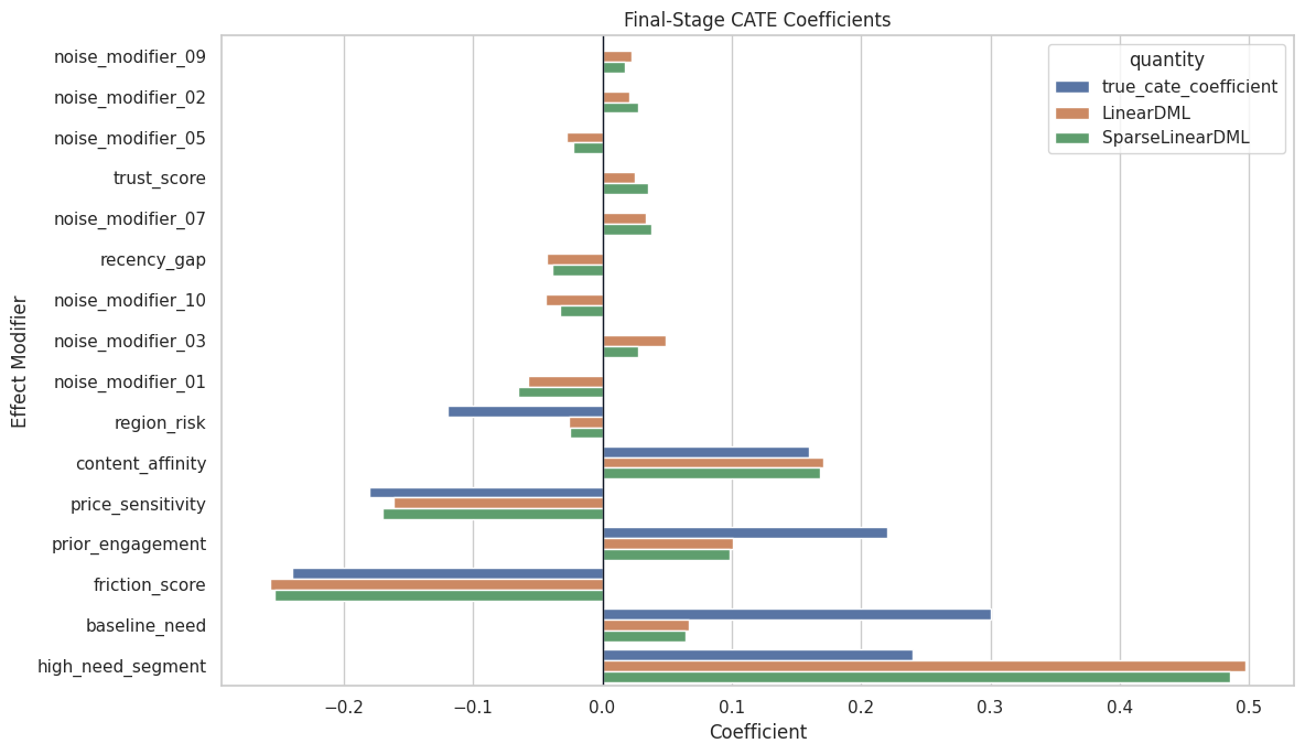
Extract Final-Stage Coefficients

For both estimators, the final-stage coefficients describe treatment-effect heterogeneity. They are not baseline outcome coefficients and they are not propensity-model coefficients.

The next cell combines the known true coefficients with the estimated coefficients from both estimators.

def extract_coef_table(estimator, estimator_name, feature_names):
    intercept = float(np.ravel(estimator.intercept_)[0])
    coefs = np.ravel(estimator.coef_)
    if len(coefs) != len(feature_names):
        raise ValueError(f"{estimator_name} returned {len(coefs)} coefficients for {len(feature_names)} features")
    return pd.DataFrame(
        {
            "term": ["cate_intercept"] + feature_names,
            estimator_name: [intercept] + list(coefs),
        }
    )

linear_coef_table = extract_coef_table(linear_dml, "LinearDML", effect_modifier_cols)
sparse_coef_table = extract_coef_table(sparse_dml, "SparseLinearDML", effect_modifier_cols)

coef_comparison = (
    true_coef_table[["term", "true_cate_coefficient", "is_true_driver"]]
    .merge(linear_coef_table, on="term", how="left")
    .merge(sparse_coef_table, on="term", how="left")
)
coef_comparison["LinearDML_abs_error"] = (coef_comparison["LinearDML"] - coef_comparison["true_cate_coefficient"]).abs()
coef_comparison["SparseLinearDML_abs_error"] = (coef_comparison["SparseLinearDML"] - coef_comparison["true_cate_coefficient"]).abs()
coef_comparison["SparseLinearDML_practically_selected"] = coef_comparison["SparseLinearDML"].abs() >= 0.03

coef_comparison.to_csv(TABLE_DIR / "03_coefficient_comparison.csv", index=False)
display(coef_comparison)

	term	true_cate_coefficient	is_true_driver	LinearDML	SparseLinearDML	LinearDML_abs_error	SparseLinearDML_abs_error	SparseLinearDML_practically_selected
0	cate_intercept	0.4200	True	0.3577	0.3684	0.0623	0.0516	True
1	baseline_need	0.3000	True	0.0668	0.0645	0.2332	0.2355	True
2	prior_engagement	0.2200	True	0.1007	0.0985	0.1193	0.1215	True
3	friction_score	-0.2400	True	-0.2569	-0.2534	0.0169	0.0134	True
4	price_sensitivity	-0.1800	True	-0.1616	-0.1701	0.0184	0.0099	True
5	content_affinity	0.1600	True	0.1708	0.1684	0.0108	0.0084	True
6	region_risk	-0.1200	True	-0.0258	-0.0254	0.0942	0.0946	False
7	high_need_segment	0.2400	True	0.4970	0.4855	0.2570	0.2455	True
8	trust_score	0.0000	False	0.0248	0.0352	0.0248	0.0352	True
9	recency_gap	0.0000	False	-0.0430	-0.0391	0.0430	0.0391	True
10	noise_modifier_01	0.0000	False	-0.0579	-0.0652	0.0579	0.0652	True
11	noise_modifier_02	0.0000	False	0.0212	0.0273	0.0212	0.0273	False
12	noise_modifier_03	0.0000	False	0.0489	0.0280	0.0489	0.0280	False
13	noise_modifier_04	0.0000	False	-0.0059	0.0049	0.0059	0.0049	False
14	noise_modifier_05	0.0000	False	-0.0281	-0.0222	0.0281	0.0222	False
15	noise_modifier_06	0.0000	False	-0.0009	0.0009	0.0009	0.0009	False
16	noise_modifier_07	0.0000	False	0.0337	0.0382	0.0337	0.0382	True
17	noise_modifier_08	0.0000	False	-0.0031	-0.0024	0.0031	0.0024	False
18	noise_modifier_09	0.0000	False	0.0223	0.0171	0.0223	0.0171	False
19	noise_modifier_10	0.0000	False	-0.0439	-0.0327	0.0439	0.0327	True
20	noise_modifier_11	0.0000	False	0.0155	0.0207	0.0155	0.0207	False
21	noise_modifier_12	0.0000	False	-0.0120	-0.0142	0.0120	0.0142	False

What this shows: coefficient tables are where linear final-stage estimators shine. They turn CATE estimation into a readable statement about which features increase or decrease treatment benefit.

Coefficient Ranking

A wide coefficient table can still be hard to scan. The next cell ranks candidate effect modifiers by absolute sparse coefficient and shows whether each one is a true CATE driver in the simulation.

ranked_coefficients = (
    coef_comparison.query("term != 'cate_intercept'")
    .assign(abs_sparse=lambda d: d["SparseLinearDML"].abs(), abs_linear=lambda d: d["LinearDML"].abs())
    .sort_values("abs_sparse", ascending=False)
    [["term", "is_true_driver", "true_cate_coefficient", "LinearDML", "SparseLinearDML", "abs_linear", "abs_sparse", "SparseLinearDML_practically_selected"]]
)

ranked_coefficients.to_csv(TABLE_DIR / "03_ranked_coefficients.csv", index=False)
display(ranked_coefficients.head(18))

	term	is_true_driver	true_cate_coefficient	LinearDML	SparseLinearDML	abs_linear	abs_sparse	SparseLinearDML_practically_selected
7	high_need_segment	True	0.2400	0.4970	0.4855	0.4970	0.4855	True
3	friction_score	True	-0.2400	-0.2569	-0.2534	0.2569	0.2534	True
4	price_sensitivity	True	-0.1800	-0.1616	-0.1701	0.1616	0.1701	True
5	content_affinity	True	0.1600	0.1708	0.1684	0.1708	0.1684	True
2	prior_engagement	True	0.2200	0.1007	0.0985	0.1007	0.0985	True
10	noise_modifier_01	False	0.0000	-0.0579	-0.0652	0.0579	0.0652	True
1	baseline_need	True	0.3000	0.0668	0.0645	0.0668	0.0645	True
9	recency_gap	False	0.0000	-0.0430	-0.0391	0.0430	0.0391	True
16	noise_modifier_07	False	0.0000	0.0337	0.0382	0.0337	0.0382	True
8	trust_score	False	0.0000	0.0248	0.0352	0.0248	0.0352	True
19	noise_modifier_10	False	0.0000	-0.0439	-0.0327	0.0439	0.0327	True
12	noise_modifier_03	False	0.0000	0.0489	0.0280	0.0489	0.0280	False
11	noise_modifier_02	False	0.0000	0.0212	0.0273	0.0212	0.0273	False
6	region_risk	True	-0.1200	-0.0258	-0.0254	0.0258	0.0254	False
14	noise_modifier_05	False	0.0000	-0.0281	-0.0222	0.0281	0.0222	False
20	noise_modifier_11	False	0.0000	0.0155	0.0207	0.0155	0.0207	False
18	noise_modifier_09	False	0.0000	0.0223	0.0171	0.0223	0.0171	False
21	noise_modifier_12	False	0.0000	-0.0120	-0.0142	0.0120	0.0142	False

What this shows: a sparse model is most useful when the top coefficients are mostly real effect drivers and the irrelevant modifiers are pushed toward small values. The exact threshold for practical selection is an analyst choice, not a universal law.

Coefficient Concentration Summary

Instead of reading every coefficient, we can summarize how much absolute coefficient mass falls on true drivers versus noise features.

coef_mass_rows = []
for estimator_name in ["LinearDML", "SparseLinearDML"]:
    temp = coef_comparison.query("term != 'cate_intercept'").copy()
    temp["abs_coef"] = temp[estimator_name].abs()
    total_abs = temp["abs_coef"].sum()
    signal_abs = temp.loc[temp["is_true_driver"], "abs_coef"].sum()
    noise_abs = temp.loc[~temp["is_true_driver"], "abs_coef"].sum()
    coef_mass_rows.append(
        {
            "estimator": estimator_name,
            "total_abs_coefficient_mass": total_abs,
            "signal_abs_coefficient_mass": signal_abs,
            "noise_abs_coefficient_mass": noise_abs,
            "signal_share_of_abs_mass": signal_abs / total_abs,
            "noise_share_of_abs_mass": noise_abs / total_abs,
            "num_practical_nonzero_abs_ge_0_03": int((temp[estimator_name].abs() >= 0.03).sum()),
        }
    )

coef_mass_summary = pd.DataFrame(coef_mass_rows)
coef_mass_summary.to_csv(TABLE_DIR / "03_coefficient_mass_summary.csv", index=False)
display(coef_mass_summary)

	estimator	total_abs_coefficient_mass	signal_abs_coefficient_mass	noise_abs_coefficient_mass	signal_share_of_abs_mass	noise_share_of_abs_mass	num_practical_nonzero_abs_ge_0_03
0	LinearDML	1.6410	1.2796	0.3613	0.7798	0.2202	11
1	SparseLinearDML	1.6139	1.2658	0.3481	0.7843	0.2157	11

What this shows: sparse estimation is not only about individual coefficients. It is also about concentrating attention on a smaller part of the candidate modifier set.

Coefficient Plot

The plot below compares true coefficients, dense LinearDML coefficients, and sparse SparseLinearDML coefficients for the most important terms. This makes sign recovery and shrinkage easier to see.

plot_terms = (
    coef_comparison.query("term != 'cate_intercept'")
    .assign(max_abs=lambda d: d[["true_cate_coefficient", "LinearDML", "SparseLinearDML"]].abs().max(axis=1))
    .sort_values("max_abs", ascending=False)
    .head(16)["term"]
    .tolist()
)

coef_plot_df = coef_comparison[coef_comparison["term"].isin(plot_terms)].melt(
    id_vars=["term", "is_true_driver"],
    value_vars=["true_cate_coefficient", "LinearDML", "SparseLinearDML"],
    var_name="quantity",
    value_name="coefficient",
)
coef_plot_df["term"] = pd.Categorical(coef_plot_df["term"], categories=plot_terms[::-1], ordered=True)

fig, ax = plt.subplots(figsize=(12, 7))
sns.barplot(
    data=coef_plot_df,
    x="coefficient",
    y="term",
    hue="quantity",
    ax=ax,
)
ax.axvline(0, color="#111827", linewidth=1)
ax.set_title("Final-Stage CATE Coefficients")
ax.set_xlabel("Coefficient")
ax.set_ylabel("Effect Modifier")
plt.tight_layout()
fig.savefig(FIGURE_DIR / "03_cate_coefficients.png", dpi=160, bbox_inches="tight")
plt.show()

What this shows: coefficient plots help communicate direction and relative size. They are most credible when paired with diagnostics about overlap, nuisance modeling, and robustness.

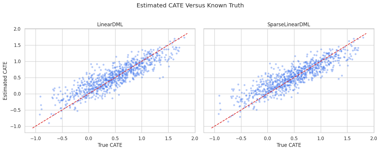
CATE Recovery Scatter

Because this is simulated data, we can compare estimated CATE to true CATE on the test set. The dashed line is perfect recovery.

cate_plot_df = pd.concat(
    [
        pd.DataFrame({"true_cate": true_cate_test, "estimated_cate": linear_cate_test, "estimator": "LinearDML"}),
        pd.DataFrame({"true_cate": true_cate_test, "estimated_cate": sparse_cate_test, "estimator": "SparseLinearDML"}),
    ],
    ignore_index=True,
)
limits = [
    min(cate_plot_df["true_cate"].min(), cate_plot_df["estimated_cate"].min()),
    max(cate_plot_df["true_cate"].max(), cate_plot_df["estimated_cate"].max()),
]

fig, axes = plt.subplots(1, 2, figsize=(13, 5), sharex=True, sharey=True)
for ax, (estimator_name, estimator_df) in zip(axes, cate_plot_df.groupby("estimator")):
    sample_df = estimator_df.sample(n=min(850, len(estimator_df)), random_state=RANDOM_SEED)
    sns.scatterplot(data=sample_df, x="true_cate", y="estimated_cate", alpha=0.35, s=22, color="#2563eb", ax=ax)
    ax.plot(limits, limits, color="#dc2626", linestyle="--", linewidth=1.5)
    ax.set_title(estimator_name)
    ax.set_xlabel("True CATE")
    ax.set_ylabel("Estimated CATE")

plt.suptitle("Estimated CATE Versus Known Truth", y=1.02)
plt.tight_layout()
fig.savefig(FIGURE_DIR / "03_cate_recovery_scatter.png", dpi=160, bbox_inches="tight")
plt.show()

What this shows: coefficient recovery and CATE recovery are related but not identical. A model can have imperfect coefficients yet still rank treatment effects reasonably well, and ranking quality is often what matters for targeting.

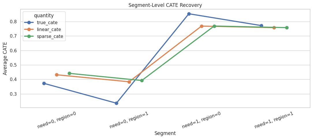
Segment-Level CATE Recovery

Segment summaries translate unit-level CATE estimates into a form that is easier to communicate. Here we summarize by high-need segment and region risk.

test_results = test_df.assign(
    linear_cate=linear_cate_test,
    sparse_cate=sparse_cate_test,
)

segment_summary = (
    test_results.groupby(["high_need_segment", "region_risk"], observed=True)
    .agg(
        rows=("outcome", "size"),
        true_cate=("true_cate", "mean"),
        linear_cate=("linear_cate", "mean"),
        sparse_cate=("sparse_cate", "mean"),
        treatment_rate=("treatment", "mean"),
        propensity_mean=("propensity", "mean"),
    )
    .reset_index()
)
segment_summary["linear_error"] = segment_summary["linear_cate"] - segment_summary["true_cate"]
segment_summary["sparse_error"] = segment_summary["sparse_cate"] - segment_summary["true_cate"]

segment_summary.to_csv(TABLE_DIR / "03_segment_cate_recovery.csv", index=False)
display(segment_summary)

	high_need_segment	region_risk	rows	true_cate	linear_cate	sparse_cate	treatment_rate	propensity_mean	linear_error	sparse_error
0	0	0	547	0.3719	0.4316	0.4414	0.3638	0.3820	0.0596	0.0694
1	0	1	240	0.2352	0.3832	0.3920	0.4542	0.4522	0.1480	0.1568
2	1	0	230	0.8535	0.7683	0.7688	0.6913	0.7115	-0.0853	-0.0847
3	1	1	103	0.7719	0.7573	0.7576	0.7670	0.7685	-0.0146	-0.0142

What this shows: segment summaries can reveal whether an estimator is useful for broad population comparisons. They also prevent us from relying only on an overall average effect.

Segment Recovery Plot

This plot compares true and estimated segment-level CATE values. Each point is a segment average.

segment_plot_df = segment_summary.melt(
    id_vars=["high_need_segment", "region_risk", "rows"],
    value_vars=["true_cate", "linear_cate", "sparse_cate"],
    var_name="quantity",
    value_name="average_cate",
)
segment_plot_df["segment"] = (
    "need=" + segment_plot_df["high_need_segment"].astype(str)
    + ", region=" + segment_plot_df["region_risk"].astype(str)
)

fig, ax = plt.subplots(figsize=(11, 5))
sns.pointplot(
    data=segment_plot_df,
    x="segment",
    y="average_cate",
    hue="quantity",
    dodge=0.35,
    errorbar=None,
    ax=ax,
)
ax.set_title("Segment-Level CATE Recovery")
ax.set_xlabel("Segment")
ax.set_ylabel("Average CATE")
ax.tick_params(axis="x", rotation=20)
plt.tight_layout()
fig.savefig(FIGURE_DIR / "03_segment_cate_recovery.png", dpi=160, bbox_inches="tight")
plt.show()

What this shows: the sparse and dense estimators should tell a similar segment story if the main heterogeneity signals are stable. Large disagreements would be a reason to inspect features, overlap, and nuisance models more carefully.

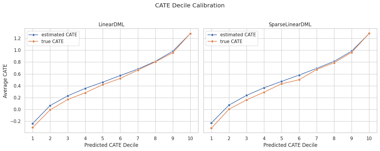
CATE Decile Calibration

For treatment targeting, ranking is often as important as exact effect magnitude. The next table groups test rows by predicted CATE decile and compares estimated versus true average CATE.

calibration_frames = []
for estimator_name, score_col in [("LinearDML", "linear_cate"), ("SparseLinearDML", "sparse_cate")]:
    temp = test_results.copy()
    temp["cate_decile"] = pd.qcut(temp[score_col], q=10, labels=False, duplicates="drop") + 1
    deciles = (
        temp.groupby("cate_decile", observed=True)
        .agg(
            rows=("outcome", "size"),
            estimated_cate=(score_col, "mean"),
            true_cate=("true_cate", "mean"),
            treatment_rate=("treatment", "mean"),
            propensity_mean=("propensity", "mean"),
        )
        .reset_index()
    )
    deciles["estimator"] = estimator_name
    calibration_frames.append(deciles)

cate_decile_calibration = pd.concat(calibration_frames, ignore_index=True)
cate_decile_calibration.to_csv(TABLE_DIR / "03_cate_decile_calibration.csv", index=False)
display(cate_decile_calibration)

	cate_decile	rows	estimated_cate	true_cate	treatment_rate	propensity_mean	estimator
0	1	112	-0.2385	-0.3054	0.3929	0.4037	LinearDML
1	2	112	0.0659	-0.0072	0.4375	0.4236	LinearDML
2	3	112	0.2293	0.1674	0.4375	0.4559	LinearDML
3	4	112	0.3555	0.2813	0.4732	0.4811	LinearDML
4	5	112	0.4601	0.4179	0.4643	0.4829	LinearDML
5	6	112	0.5723	0.5229	0.4821	0.4986	LinearDML
6	7	112	0.6812	0.6638	0.4554	0.5234	LinearDML
7	8	112	0.8120	0.8018	0.5179	0.5499	LinearDML
8	9	112	0.9832	0.9582	0.6071	0.5784	LinearDML
9	10	112	1.2821	1.2825	0.6071	0.6048	LinearDML
10	1	112	-0.2275	-0.3147	0.3929	0.4046	SparseLinearDML
11	2	112	0.0731	0.0034	0.4196	0.4291	SparseLinearDML
12	3	112	0.2370	0.1603	0.4821	0.4711	SparseLinearDML
13	4	112	0.3656	0.2914	0.4643	0.4776	SparseLinearDML
14	5	112	0.4730	0.4322	0.4732	0.4847	SparseLinearDML
15	6	112	0.5802	0.5011	0.4732	0.4891	SparseLinearDML
16	7	112	0.6928	0.6739	0.4196	0.5220	SparseLinearDML
17	8	112	0.8117	0.7890	0.5536	0.5338	SparseLinearDML
18	9	112	0.9846	0.9634	0.5804	0.5790	SparseLinearDML
19	10	112	1.2807	1.2833	0.6161	0.6115	SparseLinearDML

What this shows: a useful CATE model should produce higher true effects in higher predicted-effect deciles. In real data, we would need policy evaluation or experimental follow-up because true CATE would not be available.

CATE Decile Calibration Plot

The lines below show whether predicted CATE ranking is aligned with known true CATE ranking.

fig, axes = plt.subplots(1, 2, figsize=(13, 5), sharey=True)
for ax, (estimator_name, estimator_df) in zip(axes, cate_decile_calibration.groupby("estimator")):
    sns.lineplot(data=estimator_df, x="cate_decile", y="estimated_cate", marker="o", label="estimated CATE", ax=ax)
    sns.lineplot(data=estimator_df, x="cate_decile", y="true_cate", marker="o", label="true CATE", ax=ax)
    ax.set_title(estimator_name)
    ax.set_xlabel("Predicted CATE Decile")
    ax.set_ylabel("Average CATE")
    ax.set_xticks(sorted(estimator_df["cate_decile"].unique()))

plt.suptitle("CATE Decile Calibration", y=1.02)
plt.tight_layout()
fig.savefig(FIGURE_DIR / "03_cate_decile_calibration.png", dpi=160, bbox_inches="tight")
plt.show()

What this shows: the decile view turns CATE estimation into a ranking check. Smoothly increasing true CATE across predicted deciles means the model is learning useful prioritization structure.

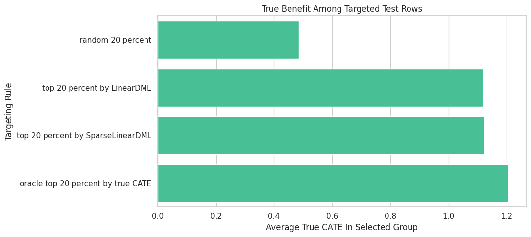
Simple Targeting Comparison

A common CATE use case is targeting the top fraction of units by estimated effect. The next cell compares three rules on the test set:

• random 20% targeting;
• top 20% by LinearDML estimated CATE;
• top 20% by SparseLinearDML estimated CATE;
• oracle top 20% by true CATE, which is only available in simulation.

targeting_fraction = 0.20
k = int(np.ceil(targeting_fraction * len(test_results)))
random_selected = test_results.sample(n=k, random_state=RANDOM_SEED).index
linear_selected = test_results.sort_values("linear_cate", ascending=False).head(k).index
sparse_selected = test_results.sort_values("sparse_cate", ascending=False).head(k).index
oracle_selected = test_results.sort_values("true_cate", ascending=False).head(k).index

targeting_rows = []
for rule_name, selected_index in [
    ("random 20 percent", random_selected),
    ("top 20 percent by LinearDML", linear_selected),
    ("top 20 percent by SparseLinearDML", sparse_selected),
    ("oracle top 20 percent by true CATE", oracle_selected),
]:
    selected = test_results.loc[selected_index]
    targeting_rows.append(
        {
            "targeting_rule": rule_name,
            "selected_rows": len(selected),
            "average_true_cate_in_selected_group": selected["true_cate"].mean(),
            "share_high_need_segment": selected["high_need_segment"].mean(),
            "share_region_risk": selected["region_risk"].mean(),
            "average_propensity": selected["propensity"].mean(),
        }
    )

targeting_summary = pd.DataFrame(targeting_rows)
targeting_summary["gain_vs_random_true_cate"] = (
    targeting_summary["average_true_cate_in_selected_group"]
    - targeting_summary.loc[targeting_summary["targeting_rule"].eq("random 20 percent"), "average_true_cate_in_selected_group"].iloc[0]
)

targeting_summary.to_csv(TABLE_DIR / "03_targeting_summary.csv", index=False)
display(targeting_summary)

	targeting_rule	selected_rows	average_true_cate_in_selected_group	share_high_need_segment	share_region_risk	average_propensity	gain_vs_random_true_cate
0	random 20 percent	224	0.4847	0.2455	0.2545	0.4969	0.0000
1	top 20 percent by LinearDML	224	1.1203	0.5714	0.2634	0.5916	0.6356
2	top 20 percent by SparseLinearDML	224	1.1233	0.5714	0.2634	0.5952	0.6386
3	oracle top 20 percent by true CATE	224	1.2063	0.6339	0.2679	0.6903	0.7215

What this shows: CATE models are often evaluated by how much better their targeted group is than random selection. The oracle row is an upper benchmark, not an achievable real-world policy.

Targeting Plot

The bar plot makes the targeting comparison easy to read: higher average true CATE in the selected group means the model is better at finding high-benefit units.

fig, ax = plt.subplots(figsize=(11, 5))
sns.barplot(
    data=targeting_summary,
    x="average_true_cate_in_selected_group",
    y="targeting_rule",
    color="#34d399",
    ax=ax,
)
ax.set_title("True Benefit Among Targeted Test Rows")
ax.set_xlabel("Average True CATE In Selected Group")
ax.set_ylabel("Targeting Rule")
plt.tight_layout()
fig.savefig(FIGURE_DIR / "03_targeting_summary.png", dpi=160, bbox_inches="tight")
plt.show()

What this shows: targeting is where CATE estimation becomes operational. Even when exact CATE values are noisy, a model can still be valuable if it ranks high-benefit units well.

Omitted Modifier Stress Test

A readable model can be too simple if it omits important effect modifiers from X. To make that risk concrete, the next cell fits a restricted LinearDML that excludes two true CATE drivers from the final stage.

The omitted variables can still be included in W for adjustment, but the final CATE model is no longer allowed to vary along them.

restricted_x_cols = [
    "baseline_need",
    "prior_engagement",
    "price_sensitivity",
    "content_affinity",
    "region_risk",
    "high_need_segment",
]
restricted_w_cols = [col for col in all_observed_covariates if col not in restricted_x_cols]

restricted_linear_dml = LinearDML(
    model_y=RandomForestRegressor(n_estimators=120, min_samples_leaf=20, random_state=RANDOM_SEED + 2, n_jobs=-1),
    model_t=RandomForestClassifier(n_estimators=120, min_samples_leaf=20, random_state=RANDOM_SEED + 2, n_jobs=-1),
    discrete_treatment=True,
    fit_cate_intercept=True,
    cv=5,
    random_state=RANDOM_SEED,
)
restricted_linear_dml.fit(
    Y_train,
    T_train,
    X=train_df[restricted_x_cols],
    W=train_df[restricted_w_cols],
    inference=None,
)
restricted_cate_test = np.ravel(restricted_linear_dml.effect(test_df[restricted_x_cols]))

restricted_comparison = pd.DataFrame(
    [
        {
            "model": "LinearDML full X",
            "num_X_features": len(effect_modifier_cols),
            "test_cate_rmse": np.sqrt(mean_squared_error(true_cate_test, linear_cate_test)),
            "test_cate_spearman": pd.Series(linear_cate_test).corr(pd.Series(true_cate_test), method="spearman"),
            "test_ate_error": linear_cate_test.mean() - true_cate_test.mean(),
        },
        {
            "model": "LinearDML restricted X",
            "num_X_features": len(restricted_x_cols),
            "test_cate_rmse": np.sqrt(mean_squared_error(true_cate_test, restricted_cate_test)),
            "test_cate_spearman": pd.Series(restricted_cate_test).corr(pd.Series(true_cate_test), method="spearman"),
            "test_ate_error": restricted_cate_test.mean() - true_cate_test.mean(),
        },
    ]
)

restricted_comparison.to_csv(TABLE_DIR / "03_restricted_x_stress_test.csv", index=False)
display(restricted_comparison)

	model	num_X_features	test_cate_rmse	test_cate_spearman	test_ate_error
0	LinearDML full X	21	0.2477	0.8760	0.0420
1	LinearDML restricted X	6	0.2719	0.8488	0.0194

What this shows: X controls what heterogeneity the final CATE model can express. Moving a true effect modifier out of X may still allow adjustment, but it prevents the reported effect from varying along that feature.

Practical Guidance Table

This table turns the notebook into a quick modeling guide for choosing between dense and sparse linear DML.

practical_guidance = pd.DataFrame(
    [
        {
            "situation": "Small number of carefully chosen effect modifiers",
            "first estimator to try": "LinearDML",
            "reason": "The final CATE coefficients are easy to read and unlikely to be cluttered.",
        },
        {
            "situation": "Many candidate modifiers, only some expected to matter",
            "first estimator to try": "SparseLinearDML",
            "reason": "Regularization can shrink weaker CATE drivers and focus the coefficient table.",
        },
        {
            "situation": "Strong nonlinear treatment-effect heterogeneity is expected",
            "first estimator to try": "CausalForestDML or another flexible estimator",
            "reason": "A linear final stage may be too restrictive even if nuisance models are flexible.",
        },
        {
            "situation": "Primary goal is a transparent segment narrative",
            "first estimator to try": "LinearDML plus segment summaries",
            "reason": "Dense coefficients and segment-level checks are usually easier to explain.",
        },
        {
            "situation": "Primary goal is treatment targeting",
            "first estimator to try": "Compare LinearDML, SparseLinearDML, and flexible CATE models",
            "reason": "Ranking quality matters; a more flexible model may rank better even if coefficients are less readable.",
        },
    ]
)

practical_guidance.to_csv(TABLE_DIR / "03_practical_guidance.csv", index=False)
display(practical_guidance)

	situation	first estimator to try	reason
0	Small number of carefully chosen effect modifiers	LinearDML	The final CATE coefficients are easy to read a...
1	Many candidate modifiers, only some expected t...	SparseLinearDML	Regularization can shrink weaker CATE drivers ...
2	Strong nonlinear treatment-effect heterogeneit...	CausalForestDML or another flexible estimator	A linear final stage may be too restrictive ev...
3	Primary goal is a transparent segment narrative	LinearDML plus segment summaries	Dense coefficients and segment-level checks ar...
4	Primary goal is treatment targeting	Compare LinearDML, SparseLinearDML, and flexib...	Ranking quality matters; a more flexible model...

What this shows: there is no universally best estimator. LinearDML and SparseLinearDML are excellent first choices when a linear CATE story is plausible, but the modeling choice should follow the causal question and expected heterogeneity pattern.

Linear DML Checklist

Before presenting a LinearDML or SparseLinearDML result, it is worth checking the items below.

linear_dml_checklist = pd.DataFrame(
    [
        {"check": "Treatment and outcome are clearly defined", "why_it_matters": "The estimator needs a precise intervention and post-treatment response."},
        {"check": "All X and W features are pre-treatment", "why_it_matters": "Post-treatment controls can distort the causal estimand."},
        {"check": "X contains the heterogeneity dimensions you want to report", "why_it_matters": "The final CATE model can vary only along X."},
        {"check": "W contains important adjustment controls", "why_it_matters": "Nuisance models need enough information to reduce confounding."},
        {"check": "Overlap is adequate", "why_it_matters": "Unsupported regions force extrapolation."},
        {"check": "Nuisance models have reasonable out-of-fold diagnostics", "why_it_matters": "Poor nuisance models leave confounding in the residuals."},
        {"check": "Coefficient signs match domain expectations where possible", "why_it_matters": "Unexpected signs can flag leakage, coding errors, or misspecification."},
        {"check": "Dense and sparse results are compared when X is wide", "why_it_matters": "Sparse shrinkage helps reveal whether the coefficient story is stable."},
        {"check": "CATE estimates are evaluated as rankings, not only point values", "why_it_matters": "Treatment targeting depends heavily on ranking quality."},
    ]
)

linear_dml_checklist.to_csv(TABLE_DIR / "03_linear_dml_checklist.csv", index=False)
display(linear_dml_checklist)

	check	why_it_matters
0	Treatment and outcome are clearly defined	The estimator needs a precise intervention and...
1	All X and W features are pre-treatment	Post-treatment controls can distort the causal...
2	X contains the heterogeneity dimensions you wa...	The final CATE model can vary only along X.
3	W contains important adjustment controls	Nuisance models need enough information to red...
4	Overlap is adequate	Unsupported regions force extrapolation.
5	Nuisance models have reasonable out-of-fold di...	Poor nuisance models leave confounding in the ...
6	Coefficient signs match domain expectations wh...	Unexpected signs can flag leakage, coding erro...
7	Dense and sparse results are compared when X i...	Sparse shrinkage helps reveal whether the coef...
8	CATE estimates are evaluated as rankings, not ...	Treatment targeting depends heavily on ranking...

What this shows: estimator output is only part of the work. A credible linear DML analysis also needs design checks, feature-role clarity, and sanity checks on the resulting CATE story.

Summary

This notebook showed how to use two readable EconML estimators for heterogeneous treatment effects.

The main takeaways are:

• LinearDML uses flexible nuisance models but keeps a linear final CATE model;
• SparseLinearDML is useful when the candidate X set is wide and only some modifiers are expected to matter;
• final-stage coefficients describe treatment-effect heterogeneity, not baseline outcome prediction;
• coefficient tables should be paired with overlap checks, nuisance diagnostics, and CATE recovery checks;
• sparse shrinkage can reduce coefficient clutter, but it can also shrink subtle real effects;
• CATE models should be evaluated both for average-effect accuracy and ranking usefulness;
• choosing X and W is a causal design decision, not just a modeling convenience.

The next tutorial can move from linear final-stage models to CausalForestDML, where the CATE surface is allowed to be nonlinear and feature importance replaces simple coefficient reading.