DoWhy Tutorial 05: Weighting, Overlap, And Common Support

This notebook focuses on the diagnostic side of propensity weighting. Inverse propensity weighting can be powerful, but it becomes fragile when treated and untreated units do not overlap. If some users are almost certain to receive treatment, or almost certain not to receive treatment, the data contain weak comparisons for those users.

We will compare two synthetic observational datasets: one with usable overlap and one with weak overlap. The causal graph and true treatment effect are the same in both cases. What changes is how separable the treated and untreated groups are.

Learning Goals

By the end of this notebook, you should be able to:

• Explain overlap, common support, and positivity in practical language.
• Estimate propensity scores and inspect treated-control overlap.
• Compute inverse propensity weights, stabilized weights, normalized IPW, and trimmed IPW estimates.
• Use effective sample size to see when weights are fragile.
• Compare raw and weighted covariate balance.
• Understand why a weighting estimator can become unstable even when the causal graph is correct.
• Run DoWhy’s propensity-score weighting estimator and read it alongside manual diagnostics.

Why Overlap Matters

Backdoor adjustment compares treated and untreated units with similar observed covariates. Propensity weighting does this by giving each unit a weight based on how surprising its observed treatment status was.

If a treated unit had a very low probability of being treated, its treated observation is rare and receives a large weight. If an untreated unit had a very high probability of being treated, its untreated observation is rare and receives a large weight. A few very large weights can dominate the estimate.

That is the practical overlap problem: the math may still run, but the estimate is supported by too few comparable observations.

Setup

This setup cell imports the packages used in the notebook, creates output folders, fixes a random seed, and suppresses known third-party compatibility warnings. The warning policy keeps expected library chatter out of the student-facing notebook while preserving real execution errors.

from pathlib import Path
import os
import platform
import sys
import warnings

START_DIR = Path.cwd().resolve()
PROJECT_ROOT = next(
    (candidate for candidate in [START_DIR, *START_DIR.parents] if (candidate / "pyproject.toml").exists()),
    START_DIR,
)

NOTEBOOK_DIR = PROJECT_ROOT / "notebooks" / "tutorials" / "dowhy"
OUTPUT_DIR = NOTEBOOK_DIR / "outputs"
FIGURE_DIR = OUTPUT_DIR / "figures"
TABLE_DIR = OUTPUT_DIR / "tables"
CACHE_DIR = PROJECT_ROOT / ".cache" / "matplotlib"

for directory in [OUTPUT_DIR, FIGURE_DIR, TABLE_DIR, CACHE_DIR]:
    directory.mkdir(parents=True, exist_ok=True)

os.environ.setdefault("MPLCONFIGDIR", str(CACHE_DIR))

warnings.filterwarnings("default")
warnings.filterwarnings("ignore", category=DeprecationWarning)
warnings.filterwarnings("ignore", category=PendingDeprecationWarning)
warnings.filterwarnings("ignore", category=FutureWarning)
warnings.filterwarnings("ignore", message=".*IProgress not found.*")
warnings.filterwarnings("ignore", message=".*setParseAction.*deprecated.*")
warnings.filterwarnings("ignore", message=".*copy keyword is deprecated.*")
warnings.filterwarnings("ignore", message=".*disp.*iprint.*L-BFGS-B.*")
warnings.filterwarnings("ignore", module="dowhy.causal_estimators.regression_estimator")
warnings.filterwarnings("ignore", module="sklearn.linear_model._logistic")
warnings.filterwarnings("ignore", module="seaborn.categorical")
warnings.filterwarnings("ignore", module="pydot.dot_parser")

import numpy as np
import pandas as pd
import matplotlib.pyplot as plt
import seaborn as sns
import statsmodels.formula.api as smf

from sklearn.linear_model import LogisticRegression
from sklearn.metrics import roc_auc_score
from sklearn.pipeline import make_pipeline
from sklearn.preprocessing import StandardScaler

import dowhy
from dowhy import CausalModel

RANDOM_SEED = 55
rng = np.random.default_rng(RANDOM_SEED)

sns.set_theme(style="whitegrid", context="notebook")

print(f"Python executable: {sys.executable}")
print(f"Python version: {platform.python_version()}")
print(f"DoWhy version: {getattr(dowhy, '__version__', 'unknown')}")
print(f"Notebook directory: {NOTEBOOK_DIR}")
print(f"Output directory: {OUTPUT_DIR}")

Python executable: /home/apex/Documents/ranking_sys/.venv/bin/python3
Python version: 3.13.12
DoWhy version: 0.14
Notebook directory: /home/apex/Documents/ranking_sys/notebooks/tutorials/dowhy
Output directory: /home/apex/Documents/ranking_sys/notebooks/tutorials/dowhy/outputs

The notebook is ready if this cell prints a DoWhy version. All generated artifacts from this notebook use a 05_ prefix.

Key Concepts

This table defines the vocabulary used throughout the notebook. These terms often appear together, but they answer slightly different diagnostic questions.

concept_table = pd.DataFrame(
    [
        {
            "concept": "Propensity score",
            "plain_language": "The probability of receiving treatment given observed covariates.",
            "why_it_matters": "It summarizes observed treatment selection into one balancing score.",
        },
        {
            "concept": "Overlap",
            "plain_language": "Treated and untreated units exist at similar covariate or propensity values.",
            "why_it_matters": "Without overlap, comparisons require extrapolation.",
        },
        {
            "concept": "Common support",
            "plain_language": "The region of propensity scores where both treatment groups are represented.",
            "why_it_matters": "Estimates outside common support are weakly supported by data.",
        },
        {
            "concept": "Positivity",
            "plain_language": "Every covariate profile has a nonzero chance of receiving each treatment level.",
            "why_it_matters": "If treatment is deterministic for some profiles, causal contrasts cannot be learned from observed data there.",
        },
        {
            "concept": "Extreme weights",
            "plain_language": "Very large inverse propensity weights from near-zero or near-one propensities.",
            "why_it_matters": "A few units can dominate the estimate and inflate variance.",
        },
        {
            "concept": "Effective sample size",
            "plain_language": "The sample size implied by the concentration of weights.",
            "why_it_matters": "A nominally large dataset can behave like a much smaller one after weighting.",
        },
    ]
)

concept_table.to_csv(TABLE_DIR / "05_weighting_concepts.csv", index=False)
concept_table

	concept	plain_language	why_it_matters
0	Propensity score	The probability of receiving treatment given o...	It summarizes observed treatment selection int...
1	Overlap	Treated and untreated units exist at similar c...	Without overlap, comparisons require extrapola...
2	Common support	The region of propensity scores where both tre...	Estimates outside common support are weakly su...
3	Positivity	Every covariate profile has a nonzero chance o...	If treatment is deterministic for some profile...
4	Extreme weights	Very large inverse propensity weights from nea...	A few units can dominate the estimate and infl...
5	Effective sample size	The sample size implied by the concentration o...	A nominally large dataset can behave like a mu...

The headline idea is simple: weighting is not only about computing a formula. It is also about checking whether the weighted comparison is supported by enough comparable observations.

Causal Question And Variable Roles

The causal question is the same in both overlap scenarios:

What is the average effect of feature_exposure on weekly_value?

The graph assumes all adjustment variables are observed pre-treatment common causes.

role_table = pd.DataFrame(
    [
        {"variable": "feature_exposure", "role": "treatment", "timing": "treatment time", "adjustment_guidance": "treatment, not a control"},
        {"variable": "weekly_value", "role": "outcome", "timing": "future outcome window", "adjustment_guidance": "outcome, not a control"},
        {"variable": "user_engagement", "role": "observed common cause", "timing": "pre-treatment", "adjustment_guidance": "adjust"},
        {"variable": "prior_sessions", "role": "observed common cause", "timing": "pre-treatment", "adjustment_guidance": "adjust"},
        {"variable": "account_age_weeks", "role": "observed common cause", "timing": "pre-treatment", "adjustment_guidance": "adjust"},
        {"variable": "is_power_user", "role": "observed common cause", "timing": "pre-treatment", "adjustment_guidance": "adjust"},
        {"variable": "baseline_value", "role": "observed common cause", "timing": "pre-treatment", "adjustment_guidance": "adjust"},
        {"variable": "true_propensity", "role": "simulation diagnostic", "timing": "known only because this is simulated", "adjustment_guidance": "do not use as a real observed column"},
    ]
)

role_table.to_csv(TABLE_DIR / "05_variable_roles.csv", index=False)
role_table

	variable	role	timing	adjustment_guidance
0	feature_exposure	treatment	treatment time	treatment, not a control
1	weekly_value	outcome	future outcome window	outcome, not a control
2	user_engagement	observed common cause	pre-treatment	adjust
3	prior_sessions	observed common cause	pre-treatment	adjust
4	account_age_weeks	observed common cause	pre-treatment	adjust
5	is_power_user	observed common cause	pre-treatment	adjust
6	baseline_value	observed common cause	pre-treatment	adjust
7	true_propensity	simulation diagnostic	known only because this is simulated	do not use as a real observed column

The same roles apply in both simulated scenarios. This is important: the graph can be correct and the adjustment set can be right, while weighting is still unstable because overlap is weak.

Create Two Overlap Scenarios

This function creates two datasets with the same outcome equation and the same true causal effect. The only difference is treatment-selection strength.

• In the usable-overlap case, baseline variables influence treatment, but not so strongly that treatment is almost deterministic.
• In the weak-overlap case, baseline variables strongly separate treated and untreated users.

def make_overlap_data(n=5_000, treatment_selection_strength=0.55, seed=55, scenario="usable_overlap"):
    local_rng = np.random.default_rng(seed)

    user_engagement = local_rng.normal(loc=0.0, scale=1.0, size=n)
    prior_sessions = np.clip(
        local_rng.poisson(lam=np.exp(1.0 + 0.20 * user_engagement), size=n),
        0,
        30,
    )
    account_age_weeks = local_rng.gamma(shape=2.2, scale=3.5, size=n)
    is_power_user = local_rng.binomial(
        n=1,
        p=1 / (1 + np.exp(-(0.75 * user_engagement - 0.20))),
        size=n,
    )
    baseline_value = (
        2.0
        + 1.00 * user_engagement
        + 0.050 * prior_sessions
        + 0.020 * account_age_weeks
        + 0.550 * is_power_user
        + local_rng.normal(loc=0.0, scale=1.0, size=n)
    )

    selection_score = (
        0.90 * user_engagement
        + 0.050 * prior_sessions
        + 0.200 * baseline_value
        + 0.550 * is_power_user
        - 0.015 * account_age_weeks
    )
    treatment_logit = -0.55 + treatment_selection_strength * selection_score
    true_propensity = 1 / (1 + np.exp(-treatment_logit))
    feature_exposure = local_rng.binomial(n=1, p=true_propensity, size=n)

    true_ate = 1.60
    weekly_value = (
        4.0
        + true_ate * feature_exposure
        + 1.20 * user_engagement
        + 0.060 * prior_sessions
        + 0.030 * account_age_weeks
        + 0.600 * baseline_value
        + 0.450 * is_power_user
        + local_rng.normal(loc=0.0, scale=1.20, size=n)
    )

    return pd.DataFrame(
        {
            "scenario": scenario,
            "feature_exposure": feature_exposure,
            "weekly_value": weekly_value,
            "user_engagement": user_engagement,
            "prior_sessions": prior_sessions,
            "account_age_weeks": account_age_weeks,
            "is_power_user": is_power_user,
            "baseline_value": baseline_value,
            "true_propensity": true_propensity,
        }
    ), true_ate

usable_df, TRUE_ATE = make_overlap_data(treatment_selection_strength=0.55, seed=55, scenario="usable_overlap")
weak_df, _ = make_overlap_data(treatment_selection_strength=2.20, seed=56, scenario="weak_overlap")

overlap_df = pd.concat([usable_df, weak_df], ignore_index=True)
overlap_df.to_csv(TABLE_DIR / "05_overlap_teaching_dataset.csv", index=False)

print(f"Rows: {len(overlap_df):,}")
print(f"Known true ATE in both scenarios: {TRUE_ATE:.4f}")
overlap_df.head()

Rows: 10,000
Known true ATE in both scenarios: 1.6000

	scenario	feature_exposure	weekly_value	user_engagement	prior_sessions	account_age_weeks	is_power_user	baseline_value	true_propensity
0	usable_overlap	1	9.855097	0.842261	1	8.283946	0	3.686182	0.557632
1	usable_overlap	1	2.480982	-2.976111	5	6.161959	0	-0.600032	0.118939
2	usable_overlap	1	6.655229	-0.305024	6	13.987074	0	2.533541	0.407891
3	usable_overlap	1	12.785204	1.449888	5	18.359764	0	4.458250	0.655687
4	usable_overlap	0	4.590193	-1.243961	2	10.443849	0	2.352953	0.281285

Both scenarios have the same true treatment effect. If estimates behave differently, the difference is coming from treatment assignment and overlap, not from a different causal effect.

Scenario Summary

This table compares treatment rates and true propensity ranges across the two scenarios.

scenario_summary = (
    overlap_df.groupby("scenario")
    .agg(
        rows=("weekly_value", "size"),
        treatment_rate=("feature_exposure", "mean"),
        outcome_mean=("weekly_value", "mean"),
        true_propensity_min=("true_propensity", "min"),
        true_propensity_p01=("true_propensity", lambda s: s.quantile(0.01)),
        true_propensity_median=("true_propensity", "median"),
        true_propensity_p99=("true_propensity", lambda s: s.quantile(0.99)),
        true_propensity_max=("true_propensity", "max"),
    )
    .reset_index()
)

scenario_summary.to_csv(TABLE_DIR / "05_scenario_summary.csv", index=False)
scenario_summary

	scenario	rows	treatment_rate	outcome_mean	true_propensity_min	true_propensity_p01	true_propensity_median	true_propensity_p99	true_propensity_max
0	usable_overlap	5000	0.4678	6.831726	0.078186	0.152451	0.464421	0.819403	0.920257
1	weak_overlap	5000	0.6260	7.164682	0.000377	0.005390	0.758453	0.999701	0.999956

The weak-overlap scenario has propensities much closer to zero and one. That means some treated or untreated observations will receive much larger inverse-propensity weights.

Estimate Propensity Scores In Each Scenario

In real observational data we do not know true propensities, so we estimate them. This cell fits a separate logistic propensity model in each scenario using the same observed common causes.

confounder_cols = ["user_engagement", "prior_sessions", "account_age_weeks", "is_power_user", "baseline_value"]

scored_parts = []
propensity_model_rows = []
for scenario, scenario_df in overlap_df.groupby("scenario"):
    X = scenario_df[confounder_cols]
    treatment = scenario_df["feature_exposure"]

    propensity_model = make_pipeline(
        StandardScaler(),
        LogisticRegression(max_iter=1_000, random_state=RANDOM_SEED),
    )
    propensity_model.fit(X, treatment)
    estimated_propensity = propensity_model.predict_proba(X)[:, 1]

    scenario_scored = scenario_df.copy()
    scenario_scored["estimated_propensity"] = estimated_propensity
    scenario_scored["clipped_propensity_01"] = np.clip(estimated_propensity, 0.01, 0.99)
    scenario_scored["clipped_propensity_05"] = np.clip(estimated_propensity, 0.05, 0.95)
    scored_parts.append(scenario_scored)

    propensity_model_rows.append(
        {
            "scenario": scenario,
            "propensity_auc": roc_auc_score(treatment, estimated_propensity),
            "estimated_propensity_min": estimated_propensity.min(),
            "estimated_propensity_p01": np.quantile(estimated_propensity, 0.01),
            "estimated_propensity_median": np.median(estimated_propensity),
            "estimated_propensity_p99": np.quantile(estimated_propensity, 0.99),
            "estimated_propensity_max": estimated_propensity.max(),
        }
    )

scored_df = pd.concat(scored_parts, ignore_index=True)
propensity_model_summary = pd.DataFrame(propensity_model_rows)

scored_df.to_csv(TABLE_DIR / "05_scored_overlap_dataset.csv", index=False)
propensity_model_summary.to_csv(TABLE_DIR / "05_propensity_model_summary.csv", index=False)
propensity_model_summary

	scenario	propensity_auc	estimated_propensity_min	estimated_propensity_p01	estimated_propensity_median	estimated_propensity_p99	estimated_propensity_max
0	usable_overlap	0.687405	0.081002	0.155716	0.460928	0.814791	0.910762
1	weak_overlap	0.917156	0.000352	0.004665	0.752000	0.999692	0.999958

The weak-overlap scenario should have a higher propensity-model AUC because treatment assignment is easier to predict. For causal weighting, easier treatment prediction often means weaker overlap.

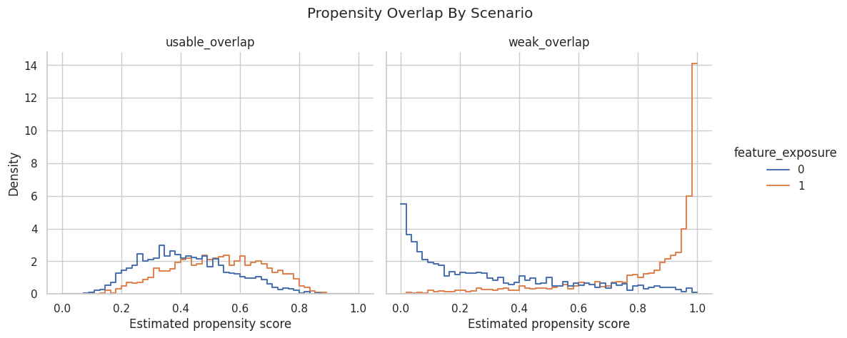
Plot Propensity Overlap

This plot compares treated and untreated propensity distributions in each scenario. Good overlap means both groups occupy similar regions of the propensity scale.

g = sns.displot(
    data=scored_df,
    x="estimated_propensity",
    hue="feature_exposure",
    col="scenario",
    bins=55,
    stat="density",
    common_norm=False,
    element="step",
    fill=False,
    height=4.5,
    aspect=1.15,
)
g.set_axis_labels("Estimated propensity score", "Density")
g.set_titles("{col_name}")
g.fig.suptitle("Propensity Overlap By Scenario", y=1.05)
g.fig.savefig(FIGURE_DIR / "05_propensity_overlap_by_scenario.png", dpi=160, bbox_inches="tight")
plt.show()

The weak-overlap panel should show more separation. That separation is the visual warning that weighting will rely on a smaller, more fragile set of comparable observations.

Common Support Diagnostics

Common support asks whether treated and untreated users exist over the same propensity range. This cell summarizes overlap using min/max ranges and the share of observations inside simple trimming bands.

def common_support_summary(df):
    rows = []
    for scenario, scenario_df in df.groupby("scenario"):
        treated_ps = scenario_df.loc[scenario_df["feature_exposure"] == 1, "estimated_propensity"]
        control_ps = scenario_df.loc[scenario_df["feature_exposure"] == 0, "estimated_propensity"]
        lower_support = max(treated_ps.min(), control_ps.min())
        upper_support = min(treated_ps.max(), control_ps.max())
        in_empirical_support = scenario_df["estimated_propensity"].between(lower_support, upper_support)
        rows.append(
            {
                "scenario": scenario,
                "treated_ps_min": treated_ps.min(),
                "treated_ps_max": treated_ps.max(),
                "control_ps_min": control_ps.min(),
                "control_ps_max": control_ps.max(),
                "empirical_common_support_lower": lower_support,
                "empirical_common_support_upper": upper_support,
                "share_inside_empirical_common_support": in_empirical_support.mean(),
                "share_inside_01_99_band": scenario_df["estimated_propensity"].between(0.01, 0.99).mean(),
                "share_inside_05_95_band": scenario_df["estimated_propensity"].between(0.05, 0.95).mean(),
                "share_inside_10_90_band": scenario_df["estimated_propensity"].between(0.10, 0.90).mean(),
            }
        )
    return pd.DataFrame(rows)

support_summary = common_support_summary(scored_df)
support_summary.to_csv(TABLE_DIR / "05_common_support_summary.csv", index=False)
support_summary

	scenario	treated_ps_min	treated_ps_max	control_ps_min	control_ps_max	empirical_common_support_lower	empirical_common_support_upper	share_inside_empirical_common_support	share_inside_01_99_band	share_inside_05_95_band	share_inside_10_90_band
0	usable_overlap	0.095802	0.910762	0.081002	0.872378	0.095802	0.872378	0.9980	1.000	1.000	0.9986
1	weak_overlap	0.023944	0.999958	0.000352	0.999121	0.023944	0.999121	0.9312	0.861	0.652	0.5194

The trimming-band shares show how much data would remain if we restricted analysis to less extreme propensity regions. Trimming improves stability, but it changes the target population.

Compute Weights And Effective Sample Size

This cell computes several weight variants:

• Plain inverse propensity weights.
• Stabilized weights, which multiply by marginal treatment probabilities.
• Clipped weights, using propensities clipped to [0.01, 0.99] and [0.05, 0.95].

It also computes effective sample size, which falls when weights concentrate on a few units.

def add_weight_columns(df):
    weighted_parts = []
    for scenario, scenario_df in df.groupby("scenario"):
        part = scenario_df.copy()
        treatment = part["feature_exposure"].to_numpy()
        p_treated = treatment.mean()

        for propensity_col, suffix in [
            ("estimated_propensity", "raw"),
            ("clipped_propensity_01", "clip01"),
            ("clipped_propensity_05", "clip05"),
        ]:
            propensity = part[propensity_col].to_numpy()
            part[f"ipw_weight_{suffix}"] = treatment / propensity + (1 - treatment) / (1 - propensity)
            part[f"stabilized_weight_{suffix}"] = (
                treatment * p_treated / propensity
                + (1 - treatment) * (1 - p_treated) / (1 - propensity)
            )
        weighted_parts.append(part)
    return pd.concat(weighted_parts, ignore_index=True)

def effective_sample_size(weights):
    weights = np.asarray(weights)
    return weights.sum() ** 2 / np.sum(weights ** 2)

weighted_df = add_weight_columns(scored_df)

weight_rows = []
for scenario, scenario_df in weighted_df.groupby("scenario"):
    for weight_col in [
        "ipw_weight_raw",
        "ipw_weight_clip01",
        "ipw_weight_clip05",
        "stabilized_weight_raw",
        "stabilized_weight_clip01",
        "stabilized_weight_clip05",
    ]:
        weights = scenario_df[weight_col]
        weight_rows.append(
            {
                "scenario": scenario,
                "weight_column": weight_col,
                "mean_weight": weights.mean(),
                "max_weight": weights.max(),
                "p95_weight": weights.quantile(0.95),
                "p99_weight": weights.quantile(0.99),
                "effective_sample_size": effective_sample_size(weights),
                "nominal_sample_size": len(weights),
                "ess_share_of_nominal": effective_sample_size(weights) / len(weights),
            }
        )

weight_diagnostics = pd.DataFrame(weight_rows)
weighted_df.to_csv(TABLE_DIR / "05_weighted_overlap_dataset.csv", index=False)
weight_diagnostics.to_csv(TABLE_DIR / "05_weight_diagnostics.csv", index=False)
weight_diagnostics

	scenario	weight_column	mean_weight	max_weight	p95_weight	p99_weight	effective_sample_size	nominal_sample_size	ess_share_of_nominal
0	usable_overlap	ipw_weight_raw	2.000951	10.438142	3.501863	4.870062	4328.470395	5000	0.865694
1	usable_overlap	ipw_weight_clip01	2.000951	10.438142	3.501863	4.870062	4328.470395	5000	0.865694
2	usable_overlap	ipw_weight_clip05	2.000951	10.438142	3.501863	4.870062	4328.470395	5000	0.865694
3	usable_overlap	stabilized_weight_raw	1.000354	4.882963	1.725269	2.411711	4357.480619	5000	0.871496
4	usable_overlap	stabilized_weight_clip01	1.000354	4.882963	1.725269	2.411711	4357.480619	5000	0.871496
5	usable_overlap	stabilized_weight_clip05	1.000354	4.882963	1.725269	2.411711	4357.480619	5000	0.871496
6	weak_overlap	ipw_weight_raw	2.093583	1138.156700	4.347776	11.870133	79.118850	5000	0.015824
7	weak_overlap	ipw_weight_clip01	1.876280	100.000000	4.347776	11.870133	1019.649847	5000	0.203930
8	weak_overlap	ipw_weight_clip05	1.771379	20.000000	4.347776	11.870133	2108.846973	5000	0.421769
9	weak_overlap	stabilized_weight_raw	1.026361	425.670606	2.179343	6.013635	132.610950	5000	0.026522
10	weak_overlap	stabilized_weight_clip01	0.945272	37.400000	2.179343	6.013635	1318.472419	5000	0.263694
11	weak_overlap	stabilized_weight_clip05	0.903971	12.520000	2.179343	6.013635	2301.196033	5000	0.460239

The weak-overlap scenario should have larger maximum weights and a smaller effective sample size. A nominal sample of thousands can behave like a much smaller sample if a few units receive huge weights.

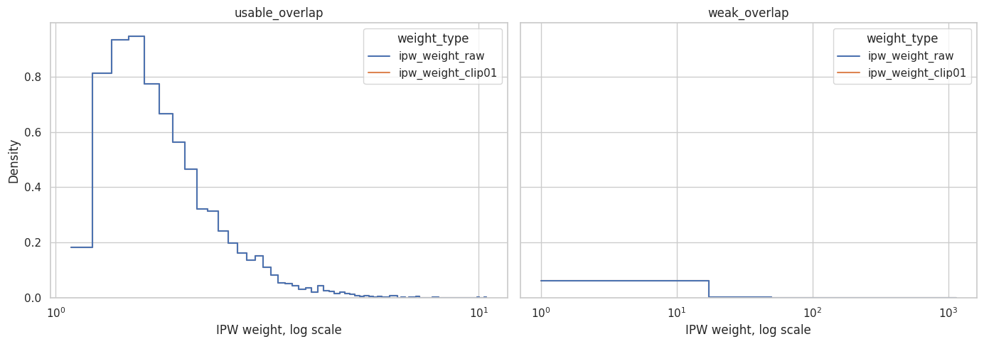
Plot Weight Distributions

Weights are easier to diagnose on a log scale because the right tail is what usually causes trouble.

weight_plot_df = weighted_df[["scenario", "feature_exposure", "ipw_weight_raw", "ipw_weight_clip01", "ipw_weight_clip05"]].melt(
    id_vars=["scenario", "feature_exposure"],
    var_name="weight_type",
    value_name="weight",
)

fig, axes = plt.subplots(1, 2, figsize=(14, 5), sharey=True)
for ax, scenario in zip(axes, ["usable_overlap", "weak_overlap"]):
    scenario_plot = weight_plot_df.query("scenario == @scenario and weight_type in ['ipw_weight_raw', 'ipw_weight_clip01']")
    sns.histplot(
        data=scenario_plot,
        x="weight",
        hue="weight_type",
        bins=70,
        stat="density",
        common_norm=False,
        element="step",
        fill=False,
        ax=ax,
    )
    ax.set_xscale("log")
    ax.set_title(scenario)
    ax.set_xlabel("IPW weight, log scale")
    ax.set_ylabel("Density")

plt.tight_layout()
fig.savefig(FIGURE_DIR / "05_weight_distributions.png", dpi=160, bbox_inches="tight")
plt.show()

The weak-overlap scenario should have a heavier right tail. Those high-weight observations are the units that make the weighting estimator more fragile.

Balance Before And After Weighting

A good weighting model should reduce imbalance in observed covariates. This cell compares raw balance to IPW-weighted balance using standardized mean differences.

def weighted_mean(values, weights):
    values = np.asarray(values)
    weights = np.asarray(weights)
    return np.sum(values * weights) / np.sum(weights)

def weighted_var(values, weights):
    values = np.asarray(values)
    weights = np.asarray(weights)
    mean = weighted_mean(values, weights)
    return np.sum(weights * (values - mean) ** 2) / np.sum(weights)

def standardized_mean_difference(df, column, weights=None):
    treatment = df["feature_exposure"].to_numpy() == 1
    values = df[column].to_numpy()
    if weights is None:
        treated_values = values[treatment]
        control_values = values[~treatment]
        pooled_sd = np.sqrt((treated_values.var(ddof=1) + control_values.var(ddof=1)) / 2)
        return (treated_values.mean() - control_values.mean()) / pooled_sd

    weights = np.asarray(weights)
    treated_mean = weighted_mean(values[treatment], weights[treatment])
    control_mean = weighted_mean(values[~treatment], weights[~treatment])
    treated_var = weighted_var(values[treatment], weights[treatment])
    control_var = weighted_var(values[~treatment], weights[~treatment])
    pooled_sd = np.sqrt((treated_var + control_var) / 2)
    return (treated_mean - control_mean) / pooled_sd

confounder_cols = ["user_engagement", "prior_sessions", "account_age_weeks", "is_power_user", "baseline_value"]

balance_rows = []
for scenario, scenario_df in weighted_df.groupby("scenario"):
    for covariate in confounder_cols:
        balance_rows.append(
            {
                "scenario": scenario,
                "covariate": covariate,
                "raw_smd": standardized_mean_difference(scenario_df, covariate),
                "weighted_smd_clip01": standardized_mean_difference(
                    scenario_df,
                    covariate,
                    weights=scenario_df["ipw_weight_clip01"].to_numpy(),
                ),
                "weighted_smd_clip05": standardized_mean_difference(
                    scenario_df,
                    covariate,
                    weights=scenario_df["ipw_weight_clip05"].to_numpy(),
                ),
            }
        )

balance_table = pd.DataFrame(balance_rows)
balance_table.to_csv(TABLE_DIR / "05_balance_before_after_weighting.csv", index=False)
balance_table

	scenario	covariate	raw_smd	weighted_smd_clip01	weighted_smd_clip05
0	usable_overlap	user_engagement	0.646501	-0.006006	-0.006006
1	usable_overlap	prior_sessions	0.264855	0.005227	0.005227
2	usable_overlap	account_age_weeks	-0.027640	-0.002722	-0.002722
3	usable_overlap	is_power_user	0.389441	-0.000155	-0.000155
4	usable_overlap	baseline_value	0.556563	-0.001766	-0.001766
5	weak_overlap	user_engagement	1.737636	0.263999	0.504594
6	weak_overlap	prior_sessions	0.502664	0.077280	0.148370
7	weak_overlap	account_age_weeks	-0.050817	0.001329	0.013894
8	weak_overlap	is_power_user	0.881697	0.161302	0.296004
9	weak_overlap	baseline_value	1.433895	0.152070	0.369736

Weighted SMDs should move toward zero if the propensity model is balancing observed covariates. Balance can improve even when weights are unstable, so balance and weight diagnostics should be read together.

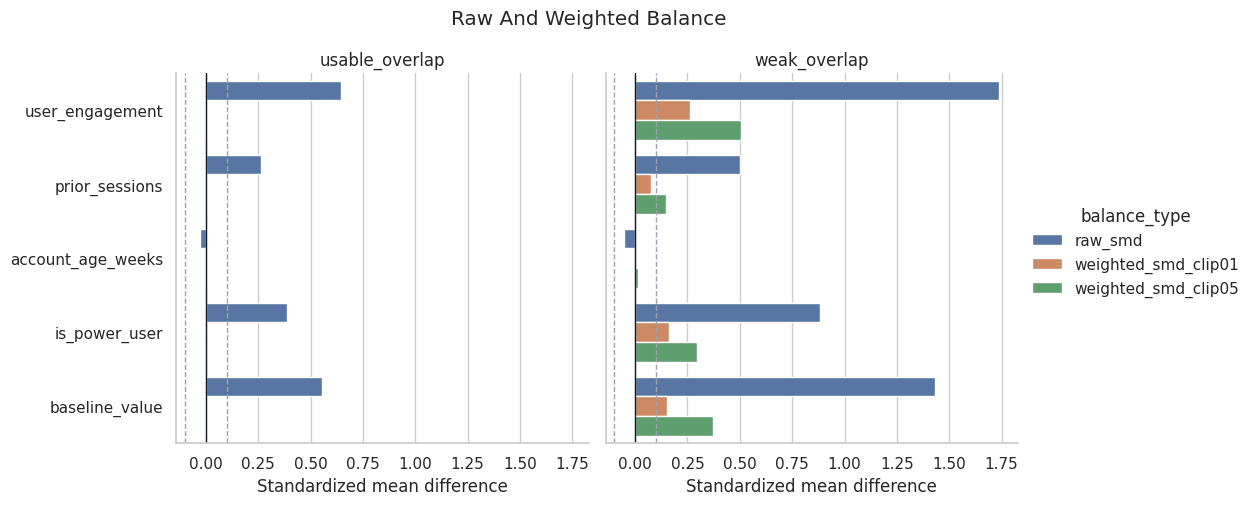
Plot Balance Diagnostics

This plot compares raw and weighted standardized mean differences across scenarios.

balance_plot_df = balance_table.melt(
    id_vars=["scenario", "covariate"],
    value_vars=["raw_smd", "weighted_smd_clip01", "weighted_smd_clip05"],
    var_name="balance_type",
    value_name="smd",
)

g = sns.catplot(
    data=balance_plot_df,
    x="smd",
    y="covariate",
    hue="balance_type",
    col="scenario",
    kind="bar",
    height=4.8,
    aspect=1.15,
    sharex=True,
)
for ax in g.axes.flat:
    ax.axvline(0, color="#111827", linewidth=1)
    ax.axvline(0.1, color="#9ca3af", linestyle="--", linewidth=1)
    ax.axvline(-0.1, color="#9ca3af", linestyle="--", linewidth=1)
g.set_axis_labels("Standardized mean difference", "")
g.set_titles("{col_name}")
g.fig.suptitle("Raw And Weighted Balance", y=1.05)
g.fig.savefig(FIGURE_DIR / "05_balance_before_after_weighting.png", dpi=160, bbox_inches="tight")
plt.show()

The weighted bars should shrink compared with the raw bars. If weighting balances covariates but the effective sample size collapses, the estimate may still be too fragile to trust without qualification.

Weighting Estimates Across Scenarios

Now we compute treatment-effect estimates for each scenario. The table includes:

• Naive treated-minus-control difference.
• Adjusted outcome regression.
• IPW using clipped propensities.
• Normalized IPW.
• Stabilized-weight outcome mean difference.
• Trimmed normalized IPW restricted to common propensity bands.

def estimate_weighted_effects(df, true_ate):
    rows = []
    for scenario, scenario_df in df.groupby("scenario"):
        treatment = scenario_df["feature_exposure"].to_numpy()
        outcome = scenario_df["weekly_value"].to_numpy()
        p01 = scenario_df["clipped_propensity_01"].to_numpy()
        p05 = scenario_df["clipped_propensity_05"].to_numpy()

        naive = scenario_df.loc[scenario_df["feature_exposure"] == 1, "weekly_value"].mean() - scenario_df.loc[
            scenario_df["feature_exposure"] == 0,
            "weekly_value",
        ].mean()

        regression_fit = smf.ols(
            formula="weekly_value ~ feature_exposure + user_engagement + prior_sessions + account_age_weeks + is_power_user + baseline_value",
            data=scenario_df,
        ).fit()
        regression_estimate = regression_fit.params["feature_exposure"]

        ipw_clip01 = np.mean(treatment * outcome / p01 - (1 - treatment) * outcome / (1 - p01))
        normalized_ipw_clip01 = (
            np.sum(treatment * outcome / p01) / np.sum(treatment / p01)
            - np.sum((1 - treatment) * outcome / (1 - p01)) / np.sum((1 - treatment) / (1 - p01))
        )

        ipw_clip05 = np.mean(treatment * outcome / p05 - (1 - treatment) * outcome / (1 - p05))
        normalized_ipw_clip05 = (
            np.sum(treatment * outcome / p05) / np.sum(treatment / p05)
            - np.sum((1 - treatment) * outcome / (1 - p05)) / np.sum((1 - treatment) / (1 - p05))
        )

        p_treated = treatment.mean()
        stabilized_weights = treatment * p_treated / p01 + (1 - treatment) * (1 - p_treated) / (1 - p01)
        stabilized_treated_mean = weighted_mean(outcome[treatment == 1], stabilized_weights[treatment == 1])
        stabilized_control_mean = weighted_mean(outcome[treatment == 0], stabilized_weights[treatment == 0])
        stabilized_difference = stabilized_treated_mean - stabilized_control_mean

        trim_mask_05_95 = scenario_df["estimated_propensity"].between(0.05, 0.95).to_numpy()
        trim_mask_10_90 = scenario_df["estimated_propensity"].between(0.10, 0.90).to_numpy()

        for estimator, estimate, rows_used in [
            ("naive_difference", naive, len(scenario_df)),
            ("adjusted_outcome_regression", regression_estimate, len(scenario_df)),
            ("ipw_clip01", ipw_clip01, len(scenario_df)),
            ("normalized_ipw_clip01", normalized_ipw_clip01, len(scenario_df)),
            ("ipw_clip05", ipw_clip05, len(scenario_df)),
            ("normalized_ipw_clip05", normalized_ipw_clip05, len(scenario_df)),
            ("stabilized_weight_difference_clip01", stabilized_difference, len(scenario_df)),
        ]:
            rows.append(
                {
                    "scenario": scenario,
                    "estimator": estimator,
                    "estimate": estimate,
                    "rows_used": rows_used,
                    "share_rows_used": rows_used / len(scenario_df),
                    "absolute_error_vs_true_ate": abs(estimate - true_ate),
                }
            )

        for trim_name, trim_mask in [("trimmed_05_95", trim_mask_05_95), ("trimmed_10_90", trim_mask_10_90)]:
            trimmed = scenario_df.loc[trim_mask].copy()
            tt = trimmed["feature_exposure"].to_numpy()
            yy = trimmed["weekly_value"].to_numpy()
            pp = trimmed["clipped_propensity_01"].to_numpy()
            trimmed_normalized_ipw = (
                np.sum(tt * yy / pp) / np.sum(tt / pp)
                - np.sum((1 - tt) * yy / (1 - pp)) / np.sum((1 - tt) / (1 - pp))
            )
            rows.append(
                {
                    "scenario": scenario,
                    "estimator": f"normalized_ipw_{trim_name}",
                    "estimate": trimmed_normalized_ipw,
                    "rows_used": len(trimmed),
                    "share_rows_used": len(trimmed) / len(scenario_df),
                    "absolute_error_vs_true_ate": abs(trimmed_normalized_ipw - true_ate),
                }
            )
    return pd.DataFrame(rows)

weighted_estimates = estimate_weighted_effects(weighted_df, TRUE_ATE)
weighted_estimates.to_csv(TABLE_DIR / "05_weighted_estimates.csv", index=False)
weighted_estimates

	scenario	estimator	estimate	rows_used	share_rows_used	absolute_error_vs_true_ate
0	usable_overlap	naive_difference	2.994493	5000	1.0000	1.394493
1	usable_overlap	adjusted_outcome_regression	1.620507	5000	1.0000	0.020507
2	usable_overlap	ipw_clip01	1.639285	5000	1.0000	0.039285
3	usable_overlap	normalized_ipw_clip01	1.612694	5000	1.0000	0.012694
4	usable_overlap	ipw_clip05	1.639285	5000	1.0000	0.039285
5	usable_overlap	normalized_ipw_clip05	1.612694	5000	1.0000	0.012694
6	usable_overlap	stabilized_weight_difference_clip01	1.612694	5000	1.0000	0.012694
7	usable_overlap	normalized_ipw_trimmed_05_95	1.612694	5000	1.0000	0.012694
8	usable_overlap	normalized_ipw_trimmed_10_90	1.615375	4993	0.9986	0.015375
9	weak_overlap	naive_difference	4.567569	5000	1.0000	2.967569
10	weak_overlap	adjusted_outcome_regression	1.683087	5000	1.0000	0.083087
11	weak_overlap	ipw_clip01	2.427237	5000	1.0000	0.827237
12	weak_overlap	normalized_ipw_clip01	2.170689	5000	1.0000	0.570689
13	weak_overlap	ipw_clip05	3.323897	5000	1.0000	1.723897
14	weak_overlap	normalized_ipw_clip05	2.646909	5000	1.0000	1.046909
15	weak_overlap	stabilized_weight_difference_clip01	2.170689	5000	1.0000	0.570689
16	weak_overlap	normalized_ipw_trimmed_05_95	1.685725	3260	0.6520	0.085725
17	weak_overlap	normalized_ipw_trimmed_10_90	1.633528	2597	0.5194	0.033528

The usable-overlap estimates should cluster closer together. In the weak-overlap case, raw weighting can drift because a few units have too much influence. Trimming often stabilizes the number, but it estimates the effect for a narrower population.

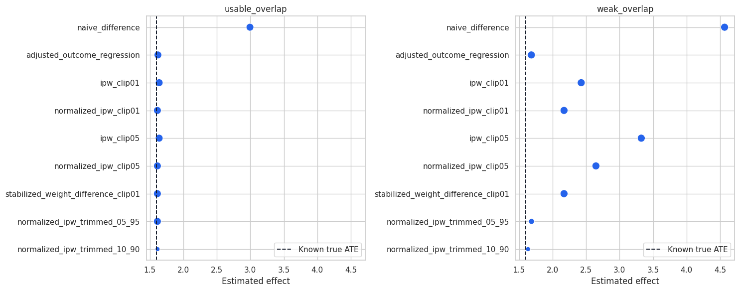
Plot Weighting Estimates

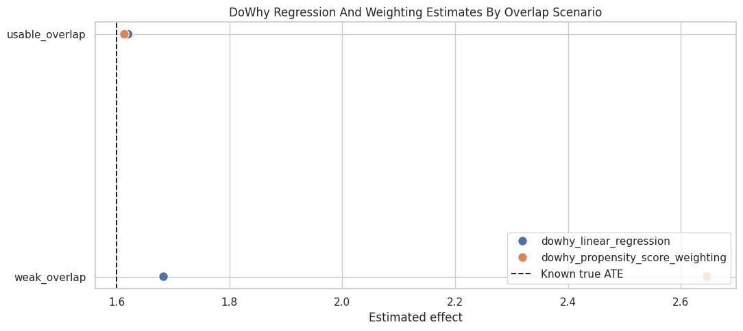
This plot compares estimators by scenario. The dashed vertical line marks the known true ATE.

fig, axes = plt.subplots(1, 2, figsize=(15, 6), sharex=True)
for ax, scenario in zip(axes, ["usable_overlap", "weak_overlap"]):
    scenario_plot = weighted_estimates.query("scenario == @scenario").copy()
    sns.scatterplot(
        data=scenario_plot,
        x="estimate",
        y="estimator",
        size="share_rows_used",
        sizes=(45, 120),
        color="#2563eb",
        legend=False,
        ax=ax,
    )
    ax.axvline(TRUE_ATE, color="#111827", linestyle="--", linewidth=1.4, label="Known true ATE")
    ax.set_title(scenario)
    ax.set_xlabel("Estimated effect")
    ax.set_ylabel("")
    ax.legend(loc="lower right")
plt.tight_layout()
fig.savefig(FIGURE_DIR / "05_weighted_estimate_comparison.png", dpi=160, bbox_inches="tight")
plt.show()

The weak-overlap panel should look less stable. The point sizes show how much data each trimmed estimator kept; trimming can reduce variance but changes the population being described.

Trimming Changes The Target Population

Trimming is not just a technical cleanup. It removes units from the tails of the propensity distribution, which often removes users with more extreme baseline profiles.

This cell summarizes how baseline covariates change after trimming.

trim_rows = []
for scenario, scenario_df in weighted_df.groupby("scenario"):
    for sample_name, mask in [
        ("full_sample", np.ones(len(scenario_df), dtype=bool)),
        ("trim_05_95", scenario_df["estimated_propensity"].between(0.05, 0.95).to_numpy()),
        ("trim_10_90", scenario_df["estimated_propensity"].between(0.10, 0.90).to_numpy()),
    ]:
        sample = scenario_df.loc[mask]
        trim_rows.append(
            {
                "scenario": scenario,
                "sample": sample_name,
                "rows": len(sample),
                "share_rows": len(sample) / len(scenario_df),
                "treatment_rate": sample["feature_exposure"].mean(),
                "mean_user_engagement": sample["user_engagement"].mean(),
                "mean_baseline_value": sample["baseline_value"].mean(),
                "mean_estimated_propensity": sample["estimated_propensity"].mean(),
            }
        )

trim_population_summary = pd.DataFrame(trim_rows)
trim_population_summary.to_csv(TABLE_DIR / "05_trimming_population_summary.csv", index=False)
trim_population_summary

	scenario	sample	rows	share_rows	treatment_rate	mean_user_engagement	mean_baseline_value	mean_estimated_propensity
0	usable_overlap	full_sample	5000	1.0000	0.467800	-0.006542	2.513019	0.467882
1	usable_overlap	trim_05_95	5000	1.0000	0.467800	-0.006542	2.513019	0.467882
2	usable_overlap	trim_10_90	4993	0.9986	0.467855	-0.004857	2.514952	0.468083
3	weak_overlap	full_sample	5000	1.0000	0.626000	0.010718	2.515658	0.626021
4	weak_overlap	trim_05_95	3260	0.6520	0.551840	-0.251799	2.142311	0.552169
5	weak_overlap	trim_10_90	2597	0.5194	0.535233	-0.279770	2.083192	0.534518

The trimmed sample may have lower or higher average baseline characteristics than the full sample. That means the trimmed estimate is often more stable but applies to a more comparable subpopulation.

DoWhy Weighting Under Usable And Weak Overlap

Now we run DoWhy’s backdoor.propensity_score_weighting estimator under the same graph in both scenarios. This connects the manual diagnostics to DoWhy’s estimator interface.

estimator_edges = [
    ("user_engagement", "feature_exposure"),
    ("user_engagement", "weekly_value"),
    ("prior_sessions", "feature_exposure"),
    ("prior_sessions", "weekly_value"),
    ("account_age_weeks", "feature_exposure"),
    ("account_age_weeks", "weekly_value"),
    ("is_power_user", "feature_exposure"),
    ("is_power_user", "weekly_value"),
    ("baseline_value", "feature_exposure"),
    ("baseline_value", "weekly_value"),
    ("feature_exposure", "weekly_value"),
]

def edges_to_dot(edges):
    lines = ["digraph {"]
    for source, target in edges:
        lines.append(f"    {source} -> {target};")
    lines.append("}")
    return chr(10).join(lines)

dowhy_graph = edges_to_dot(estimator_edges)

dowhy_rows = []
for scenario, scenario_df in overlap_df.groupby("scenario"):
    dowhy_data = scenario_df.drop(columns=["scenario", "true_propensity"]).copy()
    model = CausalModel(
        data=dowhy_data,
        treatment="feature_exposure",
        outcome="weekly_value",
        graph=dowhy_graph,
    )
    estimand = model.identify_effect(proceed_when_unidentifiable=True)
    for label, method_name in [
        ("dowhy_linear_regression", "backdoor.linear_regression"),
        ("dowhy_propensity_score_weighting", "backdoor.propensity_score_weighting"),
    ]:
        estimate = model.estimate_effect(estimand, method_name=method_name)
        dowhy_rows.append(
            {
                "scenario": scenario,
                "estimator": label,
                "method_name": method_name,
                "reported_common_causes": ", ".join(model.get_common_causes()),
                "estimate": float(estimate.value),
                "absolute_error_vs_true_ate": abs(float(estimate.value) - TRUE_ATE),
            }
        )

dowhy_weighting_comparison = pd.DataFrame(dowhy_rows)
dowhy_weighting_comparison.to_csv(TABLE_DIR / "05_dowhy_weighting_comparison.csv", index=False)
dowhy_weighting_comparison

	scenario	estimator	method_name	reported_common_causes	estimate	absolute_error_vs_true_ate
0	usable_overlap	dowhy_linear_regression	backdoor.linear_regression	is_power_user, baseline_value, user_engagement...	1.620507	0.020507
1	usable_overlap	dowhy_propensity_score_weighting	backdoor.propensity_score_weighting	is_power_user, baseline_value, user_engagement...	1.613681	0.013681
2	weak_overlap	dowhy_linear_regression	backdoor.linear_regression	is_power_user, baseline_value, user_engagement...	1.683087	0.083087
3	weak_overlap	dowhy_propensity_score_weighting	backdoor.propensity_score_weighting	is_power_user, baseline_value, user_engagement...	2.646674	1.046674

DoWhy uses the same graph in both scenarios. If the weighting estimate is less stable in the weak-overlap scenario, the issue is not graph identification; it is support and weighting fragility.

Plot DoWhy Estimates Against Manual Diagnostics

This plot shows DoWhy’s regression and weighting estimates next to the known ATE.

fig, ax = plt.subplots(figsize=(11, 5))
sns.scatterplot(
    data=dowhy_weighting_comparison,
    x="estimate",
    y="scenario",
    hue="estimator",
    s=95,
    ax=ax,
)
ax.axvline(TRUE_ATE, color="#111827", linestyle="--", linewidth=1.4, label="Known true ATE")
ax.set_title("DoWhy Regression And Weighting Estimates By Overlap Scenario")
ax.set_xlabel("Estimated effect")
ax.set_ylabel("")
ax.legend(loc="lower right")
plt.tight_layout()
fig.savefig(FIGURE_DIR / "05_dowhy_weighting_comparison.png", dpi=160, bbox_inches="tight")
plt.show()

The DoWhy weighting estimate can drift in weak overlap for the same reason manual IPW drifts: extreme propensities create extreme influence. A clean API call does not remove the need for overlap diagnostics.

Practical Decision Guide

This table summarizes what to do when weighting diagnostics look good, borderline, or poor.

decision_guide = pd.DataFrame(
    [
        {
            "diagnostic_pattern": "Good overlap, small weights, improved balance",
            "reasonable_next_step": "Report IPW or normalized IPW alongside regression and balance diagnostics.",
            "caution": "Still depends on observed-confounding assumptions.",
        },
        {
            "diagnostic_pattern": "Moderate tails but acceptable effective sample size",
            "reasonable_next_step": "Compare clipped, stabilized, and normalized weights; report sensitivity to trimming.",
            "caution": "Make clear whether trimming changes the target population.",
        },
        {
            "diagnostic_pattern": "Extreme weights and small effective sample size",
            "reasonable_next_step": "Avoid relying on raw IPW alone; consider trimming, overlap weights, redesign, or narrower estimand.",
            "caution": "The full-population ATE may not be well supported by observed data.",
        },
        {
            "diagnostic_pattern": "Balance remains poor after weighting",
            "reasonable_next_step": "Revisit the propensity model and graph assumptions before interpreting the estimate.",
            "caution": "A weighted estimate without balance is not reassuring.",
        },
    ]
)

decision_guide.to_csv(TABLE_DIR / "05_weighting_decision_guide.csv", index=False)
decision_guide

	diagnostic_pattern	reasonable_next_step	caution
0	Good overlap, small weights, improved balance	Report IPW or normalized IPW alongside regress...	Still depends on observed-confounding assumpti...
1	Moderate tails but acceptable effective sample...	Compare clipped, stabilized, and normalized we...	Make clear whether trimming changes the target...
2	Extreme weights and small effective sample size	Avoid relying on raw IPW alone; consider trimm...	The full-population ATE may not be well suppor...
3	Balance remains poor after weighting	Revisit the propensity model and graph assumpt...	A weighted estimate without balance is not rea...

This is the practical mindset: weighting is only credible when the weighted comparison is both balanced and supported by enough observations.

Final Summary

This final table gives a compact report-ready summary of the notebook’s lessons.

usable_norm = weighted_estimates.query("scenario == 'usable_overlap' and estimator == 'normalized_ipw_clip01'")["estimate"].iloc[0]
weak_norm = weighted_estimates.query("scenario == 'weak_overlap' and estimator == 'normalized_ipw_clip01'")["estimate"].iloc[0]
usable_ess = weight_diagnostics.query("scenario == 'usable_overlap' and weight_column == 'ipw_weight_clip01'")["effective_sample_size"].iloc[0]
weak_ess = weight_diagnostics.query("scenario == 'weak_overlap' and weight_column == 'ipw_weight_clip01'")["effective_sample_size"].iloc[0]

final_summary = pd.DataFrame(
    [
        {"item": "Causal question", "summary": "Average effect of feature exposure on weekly value."},
        {"item": "Known true ATE", "summary": f"{TRUE_ATE:.3f}"},
        {"item": "Usable-overlap normalized IPW", "summary": f"{usable_norm:.3f}; effective sample size about {usable_ess:.0f}."},
        {"item": "Weak-overlap normalized IPW", "summary": f"{weak_norm:.3f}; effective sample size about {weak_ess:.0f}."},
        {"item": "Main diagnostic lesson", "summary": "Weak overlap creates large weights and makes weighting estimates more fragile."},
        {"item": "Trimming lesson", "summary": "Trimming can stabilize estimates but changes the population being described."},
        {"item": "DoWhy lesson", "summary": "DoWhy can estimate weighted effects, but overlap diagnostics remain the analyst's responsibility."},
        {"item": "Main limitation", "summary": "All weighting estimators still depend on measured common causes and adequate support."},
    ]
)

final_summary.to_csv(TABLE_DIR / "05_final_weighting_summary.csv", index=False)
final_summary

	item	summary
0	Causal question	Average effect of feature exposure on weekly v...
1	Known true ATE	1.600
2	Usable-overlap normalized IPW	1.613; effective sample size about 4328.
3	Weak-overlap normalized IPW	2.171; effective sample size about 1020.
4	Main diagnostic lesson	Weak overlap creates large weights and makes w...
5	Trimming lesson	Trimming can stabilize estimates but changes t...
6	DoWhy lesson	DoWhy can estimate weighted effects, but overl...
7	Main limitation	All weighting estimators still depend on measu...

The key point is not that weighting is good or bad. Weighting is useful when the data support the comparison. When overlap is weak, the responsible answer may be a narrower estimand, a trimmed population, or a redesign of the analysis.

Student Exercises

Try these after running the notebook:

1. Increase treatment_selection_strength in the weak-overlap dataset and watch the effective sample size fall.
2. Change the clipping thresholds from [0.01, 0.99] to [0.02, 0.98] and compare estimates.
3. Compare trimming bands [0.05, 0.95], [0.10, 0.90], and [0.20, 0.80].
4. Add a nonlinear term to the propensity model and see whether balance improves.
5. Remove one confounder from the propensity model and inspect both balance and bias.
6. Write a short stakeholder summary explaining why a full-population ATE may not be supported under weak overlap.

Closing Notes

This notebook showed that inverse propensity weighting is not just a formula. It requires overlap, reasonable weights, adequate effective sample size, and improved covariate balance. The next notebook will move beyond backdoor weighting and introduce frontdoor, instrumental-variable, and natural-experiment logic.