DoWhy Tutorial 03: Backdoor Adjustment And Confounding

This notebook teaches the most common observational causal design: estimating a treatment effect after adjusting for observed common causes. The key idea is the backdoor path. A backdoor path is a noncausal path from treatment to outcome that starts by going backward into a common cause.

We will build a dataset where treatment assignment is confounded, show why the naive comparison is biased, use the causal graph to choose an adjustment set, estimate the effect with DoWhy, and then study failure cases: partial adjustment, bad controls, colliders, and unobserved confounding.

Learning Goals

By the end of this notebook, you should be able to:

• Define confounding in terms of common causes and backdoor paths.
• Explain why treated and untreated groups can differ even before treatment.
• Identify a valid adjustment set for a total-effect question.
• Estimate the same effect with manual regression and DoWhy.
• Recognize partial adjustment, mediator adjustment, collider adjustment, and unobserved confounding as different failure modes.
• Write a clear backdoor-adjustment summary with assumptions and limitations.

The Backdoor Idea In One Picture

Suppose A is treatment and Y is outcome. If a pre-treatment variable C causes both A and Y, then there is a path:

A <- C -> Y

That path creates a relationship between treatment and outcome even if treatment had no causal effect. Backdoor adjustment tries to block such paths by comparing treated and untreated units that are similar in C.

The goal is not to control for everything. The goal is to control for the right pre-treatment common causes.

Setup

This setup cell imports the packages used in the notebook, creates output folders, fixes a random seed, and suppresses known third-party compatibility warnings. It follows the same structure as the earlier DoWhy tutorials so students can focus on the causal content.

from pathlib import Path
import os
import platform
import sys
import warnings

START_DIR = Path.cwd().resolve()
PROJECT_ROOT = next(
    (candidate for candidate in [START_DIR, *START_DIR.parents] if (candidate / "pyproject.toml").exists()),
    START_DIR,
)

NOTEBOOK_DIR = PROJECT_ROOT / "notebooks" / "tutorials" / "dowhy"
OUTPUT_DIR = NOTEBOOK_DIR / "outputs"
FIGURE_DIR = OUTPUT_DIR / "figures"
TABLE_DIR = OUTPUT_DIR / "tables"
CACHE_DIR = PROJECT_ROOT / ".cache" / "matplotlib"

for directory in [OUTPUT_DIR, FIGURE_DIR, TABLE_DIR, CACHE_DIR]:
    directory.mkdir(parents=True, exist_ok=True)

os.environ.setdefault("MPLCONFIGDIR", str(CACHE_DIR))

warnings.filterwarnings("default")
warnings.filterwarnings("ignore", category=DeprecationWarning)
warnings.filterwarnings("ignore", category=PendingDeprecationWarning)
warnings.filterwarnings("ignore", category=FutureWarning)
warnings.filterwarnings("ignore", message=".*IProgress not found.*")
warnings.filterwarnings("ignore", message=".*setParseAction.*deprecated.*")
warnings.filterwarnings("ignore", message=".*copy keyword is deprecated.*")
warnings.filterwarnings("ignore", message=".*disp.*iprint.*L-BFGS-B.*")
warnings.filterwarnings("ignore", module="dowhy.causal_estimators.regression_estimator")
warnings.filterwarnings("ignore", module="sklearn.linear_model._logistic")
warnings.filterwarnings("ignore", module="seaborn.categorical")
warnings.filterwarnings("ignore", module="pydot.dot_parser")

import numpy as np
import pandas as pd
import matplotlib.pyplot as plt
import seaborn as sns
import networkx as nx
import statsmodels.formula.api as smf

import dowhy
from dowhy import CausalModel

RANDOM_SEED = 23
rng = np.random.default_rng(RANDOM_SEED)

sns.set_theme(style="whitegrid", context="notebook")

print(f"Python executable: {sys.executable}")
print(f"Python version: {platform.python_version()}")
print(f"DoWhy version: {getattr(dowhy, '__version__', 'unknown')}")
print(f"Notebook directory: {NOTEBOOK_DIR}")
print(f"Output directory: {OUTPUT_DIR}")

Python executable: /home/apex/Documents/ranking_sys/.venv/bin/python3
Python version: 3.13.12
DoWhy version: 0.14
Notebook directory: /home/apex/Documents/ranking_sys/notebooks/tutorials/dowhy
Output directory: /home/apex/Documents/ranking_sys/notebooks/tutorials/dowhy/outputs

The notebook is ready if this cell prints a DoWhy version. All outputs from this notebook use a 03_ prefix.

The Causal Question

We will use a product-style teaching example. A platform exposes some users to a feature, and we want to know whether the exposure increases future user value.

The causal question is:

What is the total average effect of feature_exposure on weekly_value?

The word total means we include all causal pathways from exposure to weekly value, including pathways through post-exposure activity.

Roles And Timing

Backdoor adjustment depends heavily on timing. This table lists each variable, when it is measured, and whether it is appropriate to adjust for when estimating the total effect.

role_table = pd.DataFrame(
    [
        {
            "variable": "feature_exposure",
            "role": "treatment",
            "timing": "treatment time",
            "total_effect_adjustment_guidance": "treatment, not a control",
        },
        {
            "variable": "weekly_value",
            "role": "outcome",
            "timing": "future outcome window",
            "total_effect_adjustment_guidance": "outcome, not a control",
        },
        {
            "variable": "user_engagement",
            "role": "observed confounder",
            "timing": "pre-treatment",
            "total_effect_adjustment_guidance": "adjust",
        },
        {
            "variable": "prior_sessions",
            "role": "observed confounder",
            "timing": "pre-treatment",
            "total_effect_adjustment_guidance": "adjust",
        },
        {
            "variable": "account_age_weeks",
            "role": "observed confounder",
            "timing": "pre-treatment",
            "total_effect_adjustment_guidance": "adjust",
        },
        {
            "variable": "baseline_value",
            "role": "observed confounder",
            "timing": "pre-treatment",
            "total_effect_adjustment_guidance": "adjust",
        },
        {
            "variable": "post_exposure_activity",
            "role": "mediator / bad control for total effect",
            "timing": "post-treatment",
            "total_effect_adjustment_guidance": "do not adjust for total effect",
        },
        {
            "variable": "support_ticket",
            "role": "collider / bad control",
            "timing": "post-treatment",
            "total_effect_adjustment_guidance": "do not adjust",
        },
        {
            "variable": "treatment_probability",
            "role": "simulation diagnostic",
            "timing": "known only because this is simulated",
            "total_effect_adjustment_guidance": "do not use as a real observed column",
        },
    ]
)

role_table.to_csv(TABLE_DIR / "03_variable_roles_and_timing.csv", index=False)
role_table

	variable	role	timing	total_effect_adjustment_guidance
0	feature_exposure	treatment	treatment time	treatment, not a control
1	weekly_value	outcome	future outcome window	outcome, not a control
2	user_engagement	observed confounder	pre-treatment	adjust
3	prior_sessions	observed confounder	pre-treatment	adjust
4	account_age_weeks	observed confounder	pre-treatment	adjust
5	baseline_value	observed confounder	pre-treatment	adjust
6	post_exposure_activity	mediator / bad control for total effect	post-treatment	do not adjust for total effect
7	support_ticket	collider / bad control	post-treatment	do not adjust
8	treatment_probability	simulation diagnostic	known only because this is simulated	do not use as a real observed column

The pre-treatment common causes are the backdoor adjustment variables. The mediator and collider are useful for teaching, but they should not be included as controls for the total effect.

Create A Confounded Dataset

This cell simulates data where the treatment effect is known. Treatment assignment depends on baseline engagement, previous sessions, account age, and baseline value. Those same variables also affect the outcome, so the naive exposed-versus-unexposed comparison will be biased.

The outcome also includes a mediated pathway through post_exposure_activity. That lets us show why controlling for a post-treatment mediator changes the estimand.

def make_backdoor_data(n=5_000, seed=23):
    local_rng = np.random.default_rng(seed)

    user_engagement = local_rng.normal(loc=0.0, scale=1.0, size=n)
    prior_sessions = np.clip(
        local_rng.poisson(lam=np.exp(1.0 + 0.25 * user_engagement), size=n),
        0,
        30,
    )
    account_age_weeks = local_rng.gamma(shape=2.0, scale=4.0, size=n)
    baseline_value = (
        2.0
        + 1.10 * user_engagement
        + 0.060 * prior_sessions
        + 0.025 * account_age_weeks
        + local_rng.normal(loc=0.0, scale=1.0, size=n)
    )

    treatment_logit = (
        -0.70
        + 0.80 * user_engagement
        + 0.040 * prior_sessions
        + 0.180 * baseline_value
        + 0.020 * account_age_weeks
    )
    treatment_probability = 1 / (1 + np.exp(-treatment_logit))
    feature_exposure = local_rng.binomial(n=1, p=treatment_probability, size=n)

    direct_effect = 1.80
    exposure_to_activity = 0.80
    activity_to_outcome = 0.50
    true_total_effect = direct_effect + exposure_to_activity * activity_to_outcome

    post_exposure_activity = (
        exposure_to_activity * feature_exposure
        + 0.70 * user_engagement
        + 0.030 * prior_sessions
        + local_rng.normal(loc=0.0, scale=1.0, size=n)
    )

    weekly_value = (
        4.0
        + direct_effect * feature_exposure
        + activity_to_outcome * post_exposure_activity
        + 1.20 * user_engagement
        + 0.060 * prior_sessions
        + 0.030 * account_age_weeks
        + 0.550 * baseline_value
        + local_rng.normal(loc=0.0, scale=1.0, size=n)
    )

    support_ticket_logit = -0.80 + 3.00 * feature_exposure - 0.50 * weekly_value + local_rng.normal(
        loc=0.0,
        scale=0.30,
        size=n,
    )
    support_ticket = local_rng.binomial(n=1, p=1 / (1 + np.exp(-support_ticket_logit)), size=n)

    df = pd.DataFrame(
        {
            "feature_exposure": feature_exposure,
            "weekly_value": weekly_value,
            "user_engagement": user_engagement,
            "prior_sessions": prior_sessions,
            "account_age_weeks": account_age_weeks,
            "baseline_value": baseline_value,
            "post_exposure_activity": post_exposure_activity,
            "support_ticket": support_ticket,
            "treatment_probability": treatment_probability,
        }
    )

    truth = {
        "direct_effect": direct_effect,
        "exposure_to_activity": exposure_to_activity,
        "activity_to_outcome": activity_to_outcome,
        "true_total_effect": true_total_effect,
    }
    return df, truth

backdoor_df, truth = make_backdoor_data()
backdoor_df.to_csv(TABLE_DIR / "03_backdoor_teaching_dataset.csv", index=False)

print(f"Rows: {len(backdoor_df):,}")
print(f"Known direct effect: {truth['direct_effect']:.4f}")
print(f"Known mediated component: {truth['exposure_to_activity'] * truth['activity_to_outcome']:.4f}")
print(f"Known total effect: {truth['true_total_effect']:.4f}")
backdoor_df.head()

Rows: 5,000
Known direct effect: 1.8000
Known mediated component: 0.4000
Known total effect: 2.2000

	feature_exposure	weekly_value	user_engagement	prior_sessions	account_age_weeks	baseline_value	post_exposure_activity	support_ticket	treatment_probability
0	1	9.413987	0.553261	1	7.155994	3.637375	1.278976	0	0.641172
1	1	10.329205	0.217601	2	21.010390	3.269387	2.433627	0	0.637095
2	1	7.837427	-0.057990	3	7.334888	3.320991	0.279148	0	0.529487
3	0	1.002724	-2.318936	1	9.944195	0.331314	-0.964946	0	0.094779
4	0	7.957376	0.431494	3	6.325859	3.002517	0.226412	0	0.606391

The generated data include the truth because this is a tutorial. In real observational data, the true effect is unknown; that is why assumptions and diagnostics matter.

Basic Dataset Summary

Before modeling, inspect treatment prevalence, outcome scale, confounder ranges, mediator scale, and collider frequency.

basic_summary = backdoor_df.agg(
    {
        "feature_exposure": ["mean", "sum"],
        "weekly_value": ["mean", "std", "min", "max"],
        "user_engagement": ["mean", "std", "min", "max"],
        "prior_sessions": ["mean", "std", "min", "max"],
        "account_age_weeks": ["mean", "std", "min", "max"],
        "baseline_value": ["mean", "std", "min", "max"],
        "post_exposure_activity": ["mean", "std", "min", "max"],
        "support_ticket": ["mean", "sum"],
        "treatment_probability": ["mean", "std", "min", "max"],
    }
).T

basic_summary.to_csv(TABLE_DIR / "03_backdoor_dataset_summary.csv")
basic_summary

	mean	sum	std	min	max
feature_exposure	0.507400	2537.0	NaN	NaN	NaN
weekly_value	6.872160	NaN	3.165655	-2.908441	18.859175
user_engagement	0.015498	NaN	1.002468	-3.859278	4.586397
prior_sessions	2.833400	NaN	1.815132	0.000000	11.000000
account_age_weeks	8.055207	NaN	5.699678	0.061549	40.820492
baseline_value	2.368113	NaN	1.529430	-3.106024	7.832728
post_exposure_activity	0.510759	NaN	1.398701	-4.455568	5.712653
support_ticket	0.111600	558.0	NaN	NaN	NaN
treatment_probability	0.502622	NaN	0.217212	0.017153	0.991037

The treatment rate is not extreme, so the data contain both exposed and unexposed units. That does not make the treatment randomized; it only means there is enough raw comparison data to proceed.

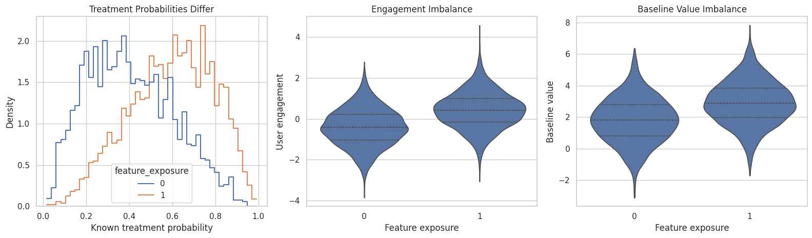
Confirm That Treatment Assignment Is Confounded

The treatment was assigned with higher probability to stronger baseline users. This plot shows imbalance in baseline variables before any outcome modeling.

fig, axes = plt.subplots(1, 3, figsize=(16, 4.8))

sns.histplot(
    data=backdoor_df,
    x="treatment_probability",
    hue="feature_exposure",
    bins=45,
    stat="density",
    common_norm=False,
    element="step",
    fill=False,
    ax=axes[0],
)
axes[0].set_title("Treatment Probabilities Differ")
axes[0].set_xlabel("Known treatment probability")
axes[0].set_ylabel("Density")

sns.violinplot(
    data=backdoor_df,
    x="feature_exposure",
    y="user_engagement",
    inner="quartile",
    cut=0,
    ax=axes[1],
)
axes[1].set_title("Engagement Imbalance")
axes[1].set_xlabel("Feature exposure")
axes[1].set_ylabel("User engagement")

sns.violinplot(
    data=backdoor_df,
    x="feature_exposure",
    y="baseline_value",
    inner="quartile",
    cut=0,
    ax=axes[2],
)
axes[2].set_title("Baseline Value Imbalance")
axes[2].set_xlabel("Feature exposure")
axes[2].set_ylabel("Baseline value")

plt.tight_layout()
fig.savefig(FIGURE_DIR / "03_confounding_assignment_checks.png", dpi=160, bbox_inches="tight")
plt.show()

The exposed group starts out stronger on baseline dimensions. If we simply compare outcomes, we will mix the treatment effect with pre-existing differences.

Quantify Baseline Imbalance

A standardized mean difference compares treated and untreated groups in standard-deviation units. It is a compact way to summarize covariate imbalance before adjustment.

def standardized_mean_difference(df, column, treatment_col="feature_exposure"):
    treated = df.loc[df[treatment_col] == 1, column]
    control = df.loc[df[treatment_col] == 0, column]
    pooled_sd = np.sqrt((treated.var(ddof=1) + control.var(ddof=1)) / 2)
    return (treated.mean() - control.mean()) / pooled_sd

baseline_columns = ["user_engagement", "prior_sessions", "account_age_weeks", "baseline_value"]
imbalance_table = pd.DataFrame(
    [
        {
            "covariate": column,
            "treated_mean": backdoor_df.loc[backdoor_df["feature_exposure"] == 1, column].mean(),
            "control_mean": backdoor_df.loc[backdoor_df["feature_exposure"] == 0, column].mean(),
            "standardized_mean_difference": standardized_mean_difference(backdoor_df, column),
        }
        for column in baseline_columns
    ]
).sort_values("standardized_mean_difference", key=lambda s: s.abs(), ascending=False)

imbalance_table.to_csv(TABLE_DIR / "03_baseline_imbalance_table.csv", index=False)
imbalance_table

	covariate	treated_mean	control_mean	standardized_mean_difference
0	user_engagement	0.425825	-0.407158	0.913207
3	baseline_value	2.913191	1.806659	0.775782
1	prior_sessions	3.212061	2.443362	0.433585
2	account_age_weeks	8.364014	7.737121	0.110195

Large absolute standardized mean differences tell us the treated and untreated groups are not directly comparable at baseline. This is the data symptom of confounding.

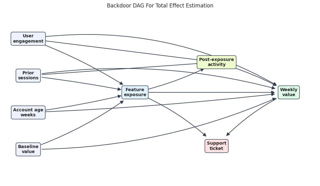
Draw The Backdoor DAG

The graph below states the causal assumptions for the total-effect question. Baseline variables cause both treatment and outcome, so they create backdoor paths. The post-exposure activity variable is a mediator, and support ticket is a collider.

backdoor_edges = [
    ("user_engagement", "feature_exposure"),
    ("user_engagement", "post_exposure_activity"),
    ("user_engagement", "weekly_value"),
    ("prior_sessions", "feature_exposure"),
    ("prior_sessions", "post_exposure_activity"),
    ("prior_sessions", "weekly_value"),
    ("account_age_weeks", "feature_exposure"),
    ("account_age_weeks", "weekly_value"),
    ("baseline_value", "feature_exposure"),
    ("baseline_value", "weekly_value"),
    ("feature_exposure", "post_exposure_activity"),
    ("post_exposure_activity", "weekly_value"),
    ("feature_exposure", "weekly_value"),
    ("feature_exposure", "support_ticket"),
    ("weekly_value", "support_ticket"),
]

node_positions = {
    "user_engagement": (0.08, 0.86),
    "prior_sessions": (0.08, 0.64),
    "account_age_weeks": (0.08, 0.42),
    "baseline_value": (0.08, 0.20),
    "feature_exposure": (0.42, 0.54),
    "post_exposure_activity": (0.68, 0.72),
    "weekly_value": (0.91, 0.54),
    "support_ticket": (0.68, 0.22),
}

node_labels = {
    "user_engagement": "User\nengagement",
    "prior_sessions": "Prior\nsessions",
    "account_age_weeks": "Account age\nweeks",
    "baseline_value": "Baseline\nvalue",
    "feature_exposure": "Feature\nexposure",
    "post_exposure_activity": "Post-exposure\nactivity",
    "weekly_value": "Weekly\nvalue",
    "support_ticket": "Support\nticket",
}

node_colors = {
    "user_engagement": "#eef2ff",
    "prior_sessions": "#eef2ff",
    "account_age_weeks": "#eef2ff",
    "baseline_value": "#eef2ff",
    "feature_exposure": "#e0f2fe",
    "post_exposure_activity": "#ecfccb",
    "weekly_value": "#dcfce7",
    "support_ticket": "#fee2e2",
}

edge_radii = {
    ("user_engagement", "feature_exposure"): -0.06,
    ("prior_sessions", "feature_exposure"): -0.02,
    ("account_age_weeks", "feature_exposure"): 0.03,
    ("baseline_value", "feature_exposure"): 0.08,
    ("user_engagement", "weekly_value"): -0.18,
    ("prior_sessions", "weekly_value"): -0.11,
    ("account_age_weeks", "weekly_value"): 0.02,
    ("baseline_value", "weekly_value"): 0.11,
    ("feature_exposure", "post_exposure_activity"): 0.07,
    ("post_exposure_activity", "weekly_value"): -0.06,
    ("feature_exposure", "weekly_value"): 0.00,
    ("feature_exposure", "support_ticket"): -0.10,
    ("weekly_value", "support_ticket"): 0.10,
}

fig, ax = plt.subplots(figsize=(13, 7))
ax.set_xlim(0, 1)
ax.set_ylim(0, 1)
ax.set_axis_off()

for source, target in backdoor_edges:
    ax.annotate(
        "",
        xy=node_positions[target],
        xytext=node_positions[source],
        arrowprops=dict(
            arrowstyle="-|>",
            color="#334155",
            linewidth=1.35,
            mutation_scale=16,
            shrinkA=32,
            shrinkB=32,
            connectionstyle=f"arc3,rad={edge_radii.get((source, target), 0.0)}",
        ),
        zorder=1,
    )

for node, (x, y) in node_positions.items():
    ax.text(
        x,
        y,
        node_labels[node],
        ha="center",
        va="center",
        fontsize=10,
        fontweight="bold",
        bbox=dict(boxstyle="round,pad=0.45", facecolor=node_colors[node], edgecolor="#334155", linewidth=1.1),
        zorder=2,
    )

ax.set_title("Backdoor DAG For Total Effect Estimation", pad=18)
fig.savefig(FIGURE_DIR / "03_backdoor_dag.png", dpi=160, bbox_inches="tight")
plt.show()

The blue baseline variables are the adjustment variables. The green mediator and red collider are downstream of treatment, so they are not part of the adjustment set for the total effect.

Path Reasoning

This table translates the graph into path-level decisions. A valid total-effect adjustment set blocks backdoor paths without blocking causal paths.

path_table = pd.DataFrame(
    [
        {
            "path": "feature_exposure <- user_engagement -> weekly_value",
            "path_type": "backdoor path",
            "action_for_total_effect": "block by adjusting for user_engagement",
        },
        {
            "path": "feature_exposure <- prior_sessions -> weekly_value",
            "path_type": "backdoor path",
            "action_for_total_effect": "block by adjusting for prior_sessions",
        },
        {
            "path": "feature_exposure <- account_age_weeks -> weekly_value",
            "path_type": "backdoor path",
            "action_for_total_effect": "block by adjusting for account_age_weeks",
        },
        {
            "path": "feature_exposure <- baseline_value -> weekly_value",
            "path_type": "backdoor path",
            "action_for_total_effect": "block by adjusting for baseline_value",
        },
        {
            "path": "feature_exposure -> weekly_value",
            "path_type": "direct causal path",
            "action_for_total_effect": "keep open",
        },
        {
            "path": "feature_exposure -> post_exposure_activity -> weekly_value",
            "path_type": "mediated causal path",
            "action_for_total_effect": "keep open for total effect",
        },
        {
            "path": "feature_exposure -> support_ticket <- weekly_value",
            "path_type": "collider path",
            "action_for_total_effect": "leave closed by not conditioning on support_ticket",
        },
    ]
)

path_table.to_csv(TABLE_DIR / "03_backdoor_path_reasoning.csv", index=False)
path_table

	path	path_type	action_for_total_effect
0	feature_exposure <- user_engagement -> weekly_...	backdoor path	block by adjusting for user_engagement
1	feature_exposure <- prior_sessions -> weekly_v...	backdoor path	block by adjusting for prior_sessions
2	feature_exposure <- account_age_weeks -> weekl...	backdoor path	block by adjusting for account_age_weeks
3	feature_exposure <- baseline_value -> weekly_v...	backdoor path	block by adjusting for baseline_value
4	feature_exposure -> weekly_value	direct causal path	keep open
5	feature_exposure -> post_exposure_activity -> ...	mediated causal path	keep open for total effect
6	feature_exposure -> support_ticket <- weekly_v...	collider path	leave closed by not conditioning on support_ti...

The adjustment set is not a list of all useful predictors. It is the set needed to block noncausal paths while preserving the causal paths that define the total effect.

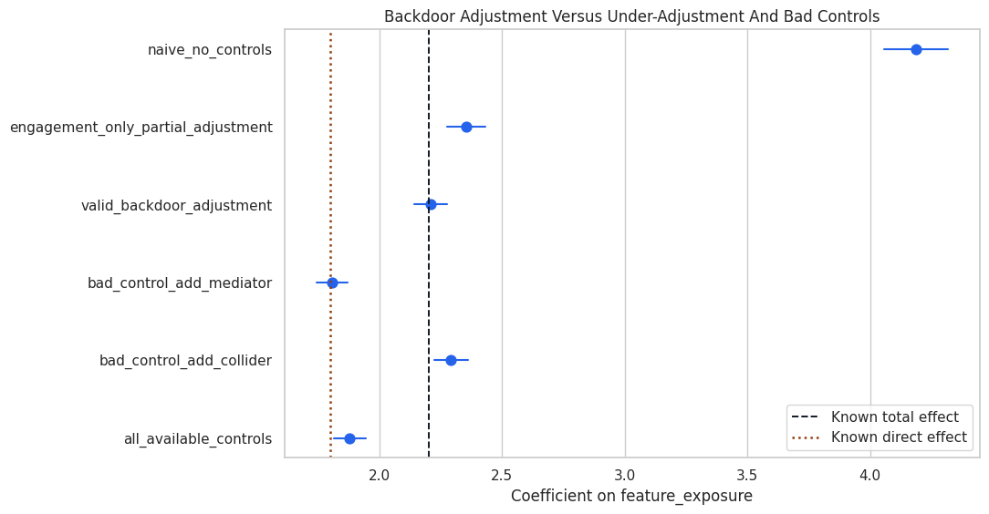
Naive Association Versus Backdoor Adjustment

We now estimate the treatment coefficient several ways. The naive model has no controls. The valid backdoor model controls for the observed pre-treatment common causes. The bad-control models add post-treatment variables that should not be included for the total effect.

formula_specs = [
    {
        "specification": "naive_no_controls",
        "formula": "weekly_value ~ feature_exposure",
        "meaning": "Association only; backdoor paths are open.",
    },
    {
        "specification": "engagement_only_partial_adjustment",
        "formula": "weekly_value ~ feature_exposure + user_engagement",
        "meaning": "Partial adjustment; some backdoor paths remain open.",
    },
    {
        "specification": "valid_backdoor_adjustment",
        "formula": "weekly_value ~ feature_exposure + user_engagement + prior_sessions + account_age_weeks + baseline_value",
        "meaning": "Total-effect estimate under observed-confounding assumptions.",
    },
    {
        "specification": "bad_control_add_mediator",
        "formula": "weekly_value ~ feature_exposure + user_engagement + prior_sessions + account_age_weeks + baseline_value + post_exposure_activity",
        "meaning": "Blocks the mediated path and moves toward a direct-effect-like quantity.",
    },
    {
        "specification": "bad_control_add_collider",
        "formula": "weekly_value ~ feature_exposure + user_engagement + prior_sessions + account_age_weeks + baseline_value + support_ticket",
        "meaning": "Conditions on a collider and can distort the total effect.",
    },
    {
        "specification": "all_available_controls",
        "formula": "weekly_value ~ feature_exposure + user_engagement + prior_sessions + account_age_weeks + baseline_value + post_exposure_activity + support_ticket",
        "meaning": "Common predictive modeling mistake: mixes confounders, mediator, and collider.",
    },
]

estimate_rows = []
for spec in formula_specs:
    fit = smf.ols(formula=spec["formula"], data=backdoor_df).fit()
    estimate = fit.params["feature_exposure"]
    ci_low, ci_high = fit.conf_int().loc["feature_exposure"].to_numpy()
    estimate_rows.append(
        {
            "specification": spec["specification"],
            "estimate": estimate,
            "ci_95_lower": ci_low,
            "ci_95_upper": ci_high,
            "distance_from_true_total": abs(estimate - truth["true_total_effect"]),
            "distance_from_true_direct": abs(estimate - truth["direct_effect"]),
            "meaning": spec["meaning"],
        }
    )

manual_estimates = pd.DataFrame(estimate_rows)
manual_estimates.to_csv(TABLE_DIR / "03_manual_backdoor_estimates.csv", index=False)
manual_estimates

	specification	estimate	ci_95_lower	ci_95_upper	distance_from_true_total	distance_from_true_direct	meaning
0	naive_no_controls	4.187805	4.056127	4.319484	1.987805	2.387805	Association only; backdoor paths are open.
1	engagement_only_partial_adjustment	2.353601	2.276337	2.430864	0.153601	0.553601	Partial adjustment; some backdoor paths remain...
2	valid_backdoor_adjustment	2.208595	2.140507	2.276682	0.008595	0.408595	Total-effect estimate under observed-confoundi...
3	bad_control_add_mediator	1.806711	1.742322	1.871100	0.393289	0.006711	Blocks the mediated path and moves toward a di...
4	bad_control_add_collider	2.290998	2.221326	2.360670	0.090998	0.490998	Conditions on a collider and can distort the t...
5	all_available_controls	1.878146	1.812068	1.944223	0.321854	0.078146	Common predictive modeling mistake: mixes conf...

The naive estimate is much larger than the total effect because baseline differences are mixed into the treatment comparison. The valid backdoor estimate should be close to the known total effect. The mediator-adjusted estimate should move toward the direct effect because part of the pathway has been controlled away.

Plot The Adjustment Results

This plot compares each specification with the known total and direct effects. It makes the consequences of under-adjustment and over-adjustment easier to see.

fig, ax = plt.subplots(figsize=(11, 5.8))
sns.pointplot(
    data=manual_estimates,
    x="estimate",
    y="specification",
    linestyle="none",
    color="#2563eb",
    ax=ax,
)
for i, row in manual_estimates.reset_index(drop=True).iterrows():
    ax.plot([row["ci_95_lower"], row["ci_95_upper"]], [i, i], color="#2563eb", linewidth=1.5)

ax.axvline(truth["true_total_effect"], color="#111827", linestyle="--", linewidth=1.4, label="Known total effect")
ax.axvline(truth["direct_effect"], color="#92400e", linestyle=":", linewidth=1.8, label="Known direct effect")
ax.set_title("Backdoor Adjustment Versus Under-Adjustment And Bad Controls")
ax.set_xlabel("Coefficient on feature_exposure")
ax.set_ylabel("")
ax.legend(loc="lower right")
plt.tight_layout()
fig.savefig(FIGURE_DIR / "03_backdoor_adjustment_estimates.png", dpi=160, bbox_inches="tight")
plt.show()

The valid backdoor specification is the one that targets the total effect. Adding more controls is not automatically better; controls must match the causal question.

Build The DoWhy Graph

Now we translate the graph into DOT syntax for DoWhy. This graph includes the confounders, the mediated pathway, and the collider, so DoWhy can reason about which variables are common causes.

def edges_to_dot(edges):
    lines = ["digraph {"]
    for source, target in edges:
        lines.append(f"    {source} -> {target};")
    lines.append("}")
    return chr(10).join(lines)

backdoor_graph = edges_to_dot(backdoor_edges)
print(backdoor_graph)

digraph {
    user_engagement -> feature_exposure;
    user_engagement -> post_exposure_activity;
    user_engagement -> weekly_value;
    prior_sessions -> feature_exposure;
    prior_sessions -> post_exposure_activity;
    prior_sessions -> weekly_value;
    account_age_weeks -> feature_exposure;
    account_age_weeks -> weekly_value;
    baseline_value -> feature_exposure;
    baseline_value -> weekly_value;
    feature_exposure -> post_exposure_activity;
    post_exposure_activity -> weekly_value;
    feature_exposure -> weekly_value;
    feature_exposure -> support_ticket;
    weekly_value -> support_ticket;
}

This graph is the formal version of the design we drew above. DoWhy will use it to identify the effect before estimating it.

Create A DoWhy CausalModel

This cell creates the DoWhy model from data, treatment, outcome, and graph. We exclude treatment_probability because that is a simulation-only diagnostic rather than an observed production variable.

model_df = backdoor_df.drop(columns=["treatment_probability"]).copy()

backdoor_model = CausalModel(
    data=model_df,
    treatment="feature_exposure",
    outcome="weekly_value",
    graph=backdoor_graph,
)

model_metadata = pd.DataFrame(
    [
        {"component": "common_causes_reported_by_DoWhy", "value": ", ".join(backdoor_model.get_common_causes())},
        {"component": "instruments_reported_by_DoWhy", "value": ", ".join(backdoor_model.get_instruments()) or "none detected"},
        {"component": "effect_modifiers_reported_by_DoWhy", "value": ", ".join(backdoor_model.get_effect_modifiers()) or "none detected"},
    ]
)

model_metadata.to_csv(TABLE_DIR / "03_dowhy_model_metadata.csv", index=False)
model_metadata

	component	value
0	common_causes_reported_by_DoWhy	baseline_value, prior_sessions, user_engagemen...
1	instruments_reported_by_DoWhy	none detected
2	effect_modifiers_reported_by_DoWhy	none detected

DoWhy reports the pre-treatment common causes. The mediator and collider are not listed as common causes, which is what we want for the total-effect question.

Identify The Backdoor Estimand

Identification asks whether the causal effect can be expressed from observed data under the graph assumptions. For this graph, DoWhy should identify a backdoor-adjustment estimand.

identified_estimand = backdoor_model.identify_effect(proceed_when_unidentifiable=True)
print(identified_estimand)

Estimand type: EstimandType.NONPARAMETRIC_ATE

### Estimand : 1
Estimand name: backdoor
Estimand expression:
        d                                                                      ↪
──────────────────(E[weekly_value|baseline_value,prior_sessions,user_engagemen ↪
d[featureₑₓₚₒₛᵤᵣₑ]                                                             ↪

↪                      
↪ t,account_age_weeks])
↪                      
Estimand assumption 1, Unconfoundedness: If U→{feature_exposure} and U→weekly_value then P(weekly_value|feature_exposure,baseline_value,prior_sessions,user_engagement,account_age_weeks,U) = P(weekly_value|feature_exposure,baseline_value,prior_sessions,user_engagement,account_age_weeks)

### Estimand : 2
Estimand name: iv
No such variable(s) found!

### Estimand : 3
Estimand name: frontdoor
No such variable(s) found!

### Estimand : 4
Estimand name: general_adjustment
Estimand expression:
        d                                                                      ↪
──────────────────(E[weekly_value|baseline_value,prior_sessions,user_engagemen ↪
d[featureₑₓₚₒₛᵤᵣₑ]                                                             ↪

↪                      
↪ t,account_age_weeks])
↪                      
Estimand assumption 1, Unconfoundedness: If U→{feature_exposure} and U→weekly_value then P(weekly_value|feature_exposure,baseline_value,prior_sessions,user_engagement,account_age_weeks,U) = P(weekly_value|feature_exposure,baseline_value,prior_sessions,user_engagement,account_age_weeks)

The printed estimand states the key assumption: after conditioning on the observed common causes, there is no remaining unobserved common cause of treatment and outcome. That assumption is not a statistical output; it is a design claim.

Estimate The Backdoor Effect With DoWhy

Now we estimate the identified estimand using DoWhy’s linear-regression estimator. In this teaching data, the graph is correct and all common causes are observed, so the estimate should be near the known total effect.

dowhy_linear_estimate = backdoor_model.estimate_effect(
    identified_estimand,
    method_name="backdoor.linear_regression",
)

print(dowhy_linear_estimate)
print(f"DoWhy backdoor estimate: {float(dowhy_linear_estimate.value):.4f}")
print(f"Known total effect: {truth['true_total_effect']:.4f}")
print(f"Known direct effect: {truth['direct_effect']:.4f}")

*** Causal Estimate ***

## Identified estimand
Estimand type: EstimandType.NONPARAMETRIC_ATE

### Estimand : 1
Estimand name: backdoor
Estimand expression:
        d                                                                      ↪
──────────────────(E[weekly_value|baseline_value,prior_sessions,user_engagemen ↪
d[featureₑₓₚₒₛᵤᵣₑ]                                                             ↪

↪                      
↪ t,account_age_weeks])
↪                      
Estimand assumption 1, Unconfoundedness: If U→{feature_exposure} and U→weekly_value then P(weekly_value|feature_exposure,baseline_value,prior_sessions,user_engagement,account_age_weeks,U) = P(weekly_value|feature_exposure,baseline_value,prior_sessions,user_engagement,account_age_weeks)

## Realized estimand
b: weekly_value~feature_exposure+baseline_value+prior_sessions+user_engagement+account_age_weeks
Target units: ate

## Estimate
Mean value: 2.208594718775249

DoWhy backdoor estimate: 2.2086
Known total effect: 2.2000
Known direct effect: 1.8000

The DoWhy estimate should align with the valid manual backdoor regression because they are using the same adjustment logic. The value is near the total effect, not the direct effect.

Compare Manual And DoWhy Estimates

This table places the manual estimates and DoWhy estimate together. It is a useful sanity check because DoWhy’s estimator should match the ordinary adjusted regression when the same linear specification is used.

dowhy_comparison = pd.concat(
    [
        manual_estimates[["specification", "estimate", "distance_from_true_total", "meaning"]],
        pd.DataFrame(
            [
                {
                    "specification": "dowhy_backdoor_linear_regression",
                    "estimate": float(dowhy_linear_estimate.value),
                    "distance_from_true_total": abs(float(dowhy_linear_estimate.value) - truth["true_total_effect"]),
                    "meaning": "DoWhy estimate after graph-based identification.",
                }
            ]
        ),
    ],
    ignore_index=True,
)

dowhy_comparison.to_csv(TABLE_DIR / "03_manual_vs_dowhy_estimates.csv", index=False)
dowhy_comparison

	specification	estimate	distance_from_true_total	meaning
0	naive_no_controls	4.187805	1.987805	Association only; backdoor paths are open.
1	engagement_only_partial_adjustment	2.353601	0.153601	Partial adjustment; some backdoor paths remain...
2	valid_backdoor_adjustment	2.208595	0.008595	Total-effect estimate under observed-confoundi...
3	bad_control_add_mediator	1.806711	0.393289	Blocks the mediated path and moves toward a di...
4	bad_control_add_collider	2.290998	0.090998	Conditions on a collider and can distort the t...
5	all_available_controls	1.878146	0.321854	Common predictive modeling mistake: mixes conf...
6	dowhy_backdoor_linear_regression	2.208595	0.008595	DoWhy estimate after graph-based identification.

The main lesson is not that DoWhy gives a different regression coefficient. The lesson is that DoWhy wraps the coefficient in a graph, an estimand, and a set of assumptions.

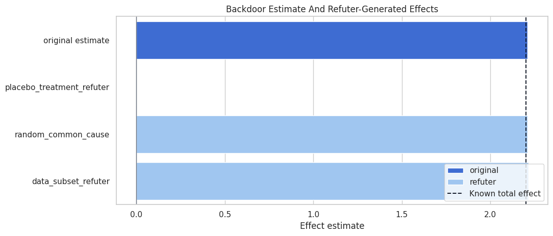
Refute The Backdoor Estimate

Refuters are stress tests. They do not prove the causal effect is correct, but they help catch estimates that behave strangely under simple perturbations.

def scalar_or_nan(value):
    try:
        return float(np.asarray(value).reshape(-1)[0])
    except Exception:
        return np.nan

refuter_specs = [
    (
        "placebo_treatment_refuter",
        {
            "method_name": "placebo_treatment_refuter",
            "placebo_type": "permute",
            "num_simulations": 20,
        },
        "A fake treatment should not reproduce the original effect.",
    ),
    (
        "random_common_cause",
        {
            "method_name": "random_common_cause",
            "num_simulations": 20,
        },
        "Adding a random irrelevant common cause should not materially change the effect.",
    ),
    (
        "data_subset_refuter",
        {
            "method_name": "data_subset_refuter",
            "subset_fraction": 0.80,
            "num_simulations": 20,
        },
        "Random subsets should produce estimates in the same neighborhood.",
    ),
]

refuter_rows = []
for label, kwargs, expected_behavior in refuter_specs:
    result = backdoor_model.refute_estimate(identified_estimand, dowhy_linear_estimate, **kwargs)
    payload = getattr(result, "refutation_result", None)
    p_value = np.nan
    if isinstance(payload, dict):
        p_value = scalar_or_nan(payload.get("p_value"))
    new_effect = scalar_or_nan(result.new_effect)
    estimated_effect = scalar_or_nan(result.estimated_effect)
    refuter_rows.append(
        {
            "refuter": label,
            "estimated_effect": estimated_effect,
            "new_effect": new_effect,
            "effect_shift": new_effect - estimated_effect,
            "p_value": p_value,
            "expected_behavior": expected_behavior,
        }
    )

refuter_summary = pd.DataFrame(refuter_rows)
refuter_summary.to_csv(TABLE_DIR / "03_refuter_summary.csv", index=False)
refuter_summary

	refuter	estimated_effect	new_effect	effect_shift	p_value	expected_behavior
0	placebo_treatment_refuter	2.208595	-0.001197	-2.209791	0.486609	A fake treatment should not reproduce the orig...
1	random_common_cause	2.208595	2.208530	-0.000065	0.393349	Adding a random irrelevant common cause should...
2	data_subset_refuter	2.208595	2.213936	0.005341	0.367017	Random subsets should produce estimates in the...

The placebo result should move toward zero, while the random-common-cause and subset checks should stay close to the original estimate. These are basic checks, not a replacement for thinking carefully about unobserved confounding.

Visualize Refuter Results

This plot shows the original estimate next to the refuter-generated effects.

refuter_plot_df = pd.concat(
    [
        pd.DataFrame(
            [
                {
                    "label": "original estimate",
                    "effect": float(dowhy_linear_estimate.value),
                    "type": "original",
                }
            ]
        ),
        refuter_summary.assign(label=refuter_summary["refuter"], effect=refuter_summary["new_effect"], type="refuter")[
            ["label", "effect", "type"]
        ],
    ],
    ignore_index=True,
)

fig, ax = plt.subplots(figsize=(11, 4.8))
sns.barplot(
    data=refuter_plot_df,
    x="effect",
    y="label",
    hue="type",
    dodge=False,
    palette={"original": "#2563eb", "refuter": "#93c5fd"},
    ax=ax,
)
ax.axvline(0, color="#6b7280", linewidth=1)
ax.axvline(truth["true_total_effect"], color="#111827", linestyle="--", linewidth=1.4, label="Known total effect")
ax.set_title("Backdoor Estimate And Refuter-Generated Effects")
ax.set_xlabel("Effect estimate")
ax.set_ylabel("")
ax.legend(loc="lower right")
plt.tight_layout()
fig.savefig(FIGURE_DIR / "03_refuter_results.png", dpi=160, bbox_inches="tight")
plt.show()

The refuter plot should show a clear separation between the original effect and the placebo effect. Stable subset and random-common-cause results are reassuring, but they do not test every possible source of bias.

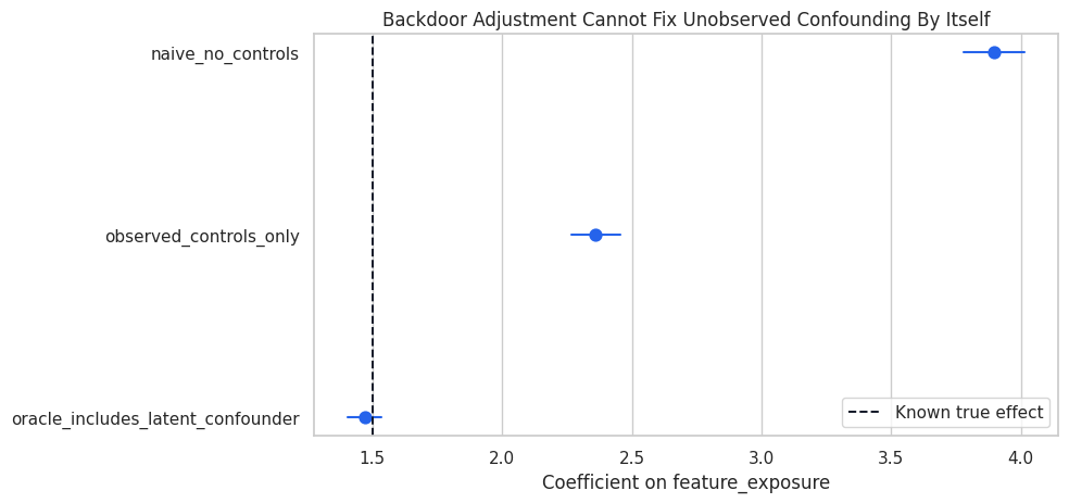
What If A Confounder Is Unobserved?

Backdoor adjustment only works if the important common causes are observed and measured well enough. This section creates a second dataset with a latent confounder. We will compare naive adjustment, observed-only adjustment, and an oracle adjustment that includes the latent variable.

The oracle model is not available in real work. It is included only to show what unobserved confounding can do.

def make_hidden_confounding_data(n=5_000, seed=91):
    local_rng = np.random.default_rng(seed)
    latent_motivation = local_rng.normal(loc=0.0, scale=1.0, size=n)
    proxy_engagement = 0.60 * latent_motivation + local_rng.normal(loc=0.0, scale=1.0, size=n)
    prior_sessions = np.clip(
        local_rng.poisson(lam=np.exp(1.0 + 0.20 * proxy_engagement), size=n),
        0,
        25,
    )

    treatment_logit = -0.40 + 0.70 * proxy_engagement + 0.050 * prior_sessions + 1.00 * latent_motivation
    treatment_probability = 1 / (1 + np.exp(-treatment_logit))
    feature_exposure = local_rng.binomial(n=1, p=treatment_probability, size=n)

    true_effect = 1.50
    weekly_value = (
        3.0
        + true_effect * feature_exposure
        + 0.90 * proxy_engagement
        + 0.050 * prior_sessions
        + 1.40 * latent_motivation
        + local_rng.normal(loc=0.0, scale=1.0, size=n)
    )

    df = pd.DataFrame(
        {
            "feature_exposure": feature_exposure,
            "weekly_value": weekly_value,
            "proxy_engagement": proxy_engagement,
            "prior_sessions": prior_sessions,
            "latent_motivation": latent_motivation,
            "treatment_probability": treatment_probability,
        }
    )
    return df, true_effect

hidden_df, hidden_true_effect = make_hidden_confounding_data()

hidden_estimates = []
for specification, formula, meaning in [
    ("naive_no_controls", "weekly_value ~ feature_exposure", "No confounding adjustment."),
    (
        "observed_controls_only",
        "weekly_value ~ feature_exposure + proxy_engagement + prior_sessions",
        "Uses observed proxy variables but omits latent motivation.",
    ),
    (
        "oracle_includes_latent_confounder",
        "weekly_value ~ feature_exposure + proxy_engagement + prior_sessions + latent_motivation",
        "Only possible in simulation; shows what would happen if the latent confounder were observed.",
    ),
]:
    fit = smf.ols(formula=formula, data=hidden_df).fit()
    estimate = fit.params["feature_exposure"]
    ci_low, ci_high = fit.conf_int().loc["feature_exposure"].to_numpy()
    hidden_estimates.append(
        {
            "specification": specification,
            "estimate": estimate,
            "ci_95_lower": ci_low,
            "ci_95_upper": ci_high,
            "distance_from_true_effect": abs(estimate - hidden_true_effect),
            "meaning": meaning,
        }
    )

hidden_confounding_results = pd.DataFrame(hidden_estimates)
hidden_confounding_results.to_csv(TABLE_DIR / "03_hidden_confounding_results.csv", index=False)
hidden_confounding_results

	specification	estimate	ci_95_lower	ci_95_upper	distance_from_true_effect	meaning
0	naive_no_controls	3.896750	3.780466	4.013034	2.396750	No confounding adjustment.
1	observed_controls_only	2.360954	2.267349	2.454560	0.860954	Uses observed proxy variables but omits latent...
2	oracle_includes_latent_confounder	1.470193	1.404429	1.535957	0.029807	Only possible in simulation; shows what would ...

Observed controls help, but they do not fully remove bias when an important common cause is unobserved. The oracle row shows why measurement matters: a valid adjustment set is not just a graph idea; it requires actual columns that measure the relevant causes.

Visualize Hidden Confounding

This plot compares the hidden-confounding estimates to the true effect from the simulation.

fig, ax = plt.subplots(figsize=(10, 4.8))
sns.pointplot(
    data=hidden_confounding_results,
    x="estimate",
    y="specification",
    linestyle="none",
    color="#2563eb",
    ax=ax,
)
for i, row in hidden_confounding_results.reset_index(drop=True).iterrows():
    ax.plot([row["ci_95_lower"], row["ci_95_upper"]], [i, i], color="#2563eb", linewidth=1.5)

ax.axvline(hidden_true_effect, color="#111827", linestyle="--", linewidth=1.4, label="Known true effect")
ax.set_title("Backdoor Adjustment Cannot Fix Unobserved Confounding By Itself")
ax.set_xlabel("Coefficient on feature_exposure")
ax.set_ylabel("")
ax.legend(loc="lower right")
plt.tight_layout()
fig.savefig(FIGURE_DIR / "03_hidden_confounding_results.png", dpi=160, bbox_inches="tight")
plt.show()

The observed-only model remains biased because the true common cause is not fully measured. This is why causal reports should say “under observed-confounding assumptions” rather than pretending adjustment is automatic proof.

Assumption Register

A backdoor analysis should document its assumptions plainly. This table turns the graph into reviewable claims.

assumption_register = pd.DataFrame(
    [
        {
            "assumption": "All major common causes of exposure and weekly value are measured.",
            "why_it_matters": "Backdoor adjustment fails if important common causes are missing.",
            "diagnostic_or_response": "Use domain review, pre-treatment covariate audits, sensitivity checks, and negative controls where possible.",
        },
        {
            "assumption": "Adjustment variables are pre-treatment.",
            "why_it_matters": "Post-treatment controls can block causal pathways or open collider paths.",
            "diagnostic_or_response": "Create a variable timing table before modeling.",
        },
        {
            "assumption": "The chosen covariates block backdoor paths without blocking the total-effect pathway.",
            "why_it_matters": "The estimand should match the causal question.",
            "diagnostic_or_response": "Write path reasoning before estimating the effect.",
        },
        {
            "assumption": "There is adequate overlap across treatment groups after adjustment.",
            "why_it_matters": "Adjustment becomes unstable when comparable controls or treated units are absent.",
            "diagnostic_or_response": "Inspect propensity overlap and common support in a dedicated weighting/overlap analysis.",
        },
        {
            "assumption": "The outcome model is adequate for the estimator being used.",
            "why_it_matters": "A valid estimand can still be estimated poorly by a misspecified model.",
            "diagnostic_or_response": "Compare estimators and inspect residual/model diagnostics.",
        },
    ]
)

assumption_register.to_csv(TABLE_DIR / "03_backdoor_assumption_register.csv", index=False)
assumption_register

	assumption	why_it_matters	diagnostic_or_response
0	All major common causes of exposure and weekly...	Backdoor adjustment fails if important common ...	Use domain review, pre-treatment covariate aud...
1	Adjustment variables are pre-treatment.	Post-treatment controls can block causal pathw...	Create a variable timing table before modeling.
2	The chosen covariates block backdoor paths wit...	The estimand should match the causal question.	Write path reasoning before estimating the eff...
3	There is adequate overlap across treatment gro...	Adjustment becomes unstable when comparable co...	Inspect propensity overlap and common support ...
4	The outcome model is adequate for the estimato...	A valid estimand can still be estimated poorly...	Compare estimators and inspect residual/model ...

This table is the honest part of the analysis. It tells a reader where the result is strongest and where judgment or additional diagnostics are still needed.

Final Backdoor Checklist

This checklist is a reusable workflow for backdoor adjustment in future notebooks.

backdoor_checklist = pd.DataFrame(
    [
        {
            "step": "Define treatment and outcome",
            "question_to_answer": "What intervention and outcome window are being compared?",
        },
        {
            "step": "Mark timing",
            "question_to_answer": "Which variables are definitely measured before treatment?",
        },
        {
            "step": "Draw common causes",
            "question_to_answer": "Which pre-treatment variables plausibly cause both treatment and outcome?",
        },
        {
            "step": "Avoid bad controls",
            "question_to_answer": "Are any proposed controls mediators, colliders, or descendants of treatment?",
        },
        {
            "step": "Check baseline imbalance",
            "question_to_answer": "How different are treated and untreated users before treatment?",
        },
        {
            "step": "Identify with DoWhy",
            "question_to_answer": "What adjustment set and assumptions does DoWhy print?",
        },
        {
            "step": "Estimate and compare",
            "question_to_answer": "How do naive, partial, valid, and bad-control estimates differ?",
        },
        {
            "step": "Run refuters",
            "question_to_answer": "Does the estimate behave sensibly under placebo and perturbation checks?",
        },
        {
            "step": "State limitations",
            "question_to_answer": "Which unobserved confounders or measurement gaps could still bias the result?",
        },
    ]
)

backdoor_checklist.to_csv(TABLE_DIR / "03_backdoor_checklist.csv", index=False)
backdoor_checklist

	step	question_to_answer
0	Define treatment and outcome	What intervention and outcome window are being...
1	Mark timing	Which variables are definitely measured before...
2	Draw common causes	Which pre-treatment variables plausibly cause ...
3	Avoid bad controls	Are any proposed controls mediators, colliders...
4	Check baseline imbalance	How different are treated and untreated users ...
5	Identify with DoWhy	What adjustment set and assumptions does DoWhy...
6	Estimate and compare	How do naive, partial, valid, and bad-control ...
7	Run refuters	Does the estimate behave sensibly under placeb...
8	State limitations	Which unobserved confounders or measurement ga...

The checklist makes backdoor adjustment less mysterious. The hard part is not calling an estimator; the hard part is defending the adjustment set.

Final Causal Summary

This final table shows how to summarize the tutorial result without overclaiming.

final_summary = pd.DataFrame(
    [
        {
            "item": "Causal question",
            "summary": "Total average effect of feature exposure on weekly value.",
        },
        {
            "item": "Valid adjustment variables in this teaching graph",
            "summary": "user_engagement, prior_sessions, account_age_weeks, and baseline_value.",
        },
        {
            "item": "Known total effect",
            "summary": f"{truth['true_total_effect']:.3f}",
        },
        {
            "item": "DoWhy backdoor estimate",
            "summary": f"{float(dowhy_linear_estimate.value):.3f}",
        },
        {
            "item": "What the naive estimate does wrong",
            "summary": "It mixes treatment effect with baseline differences between exposed and unexposed users.",
        },
        {
            "item": "What mediator adjustment does wrong for total effect",
            "summary": "It blocks part of the causal pathway and moves toward a direct-effect-like quantity.",
        },
        {
            "item": "What collider adjustment can do wrong",
            "summary": "It can open a noncausal path between treatment and outcome.",
        },
        {
            "item": "Main limitation",
            "summary": "Backdoor adjustment depends on measured common causes; unobserved confounding can remain.",
        },
    ]
)

final_summary.to_csv(TABLE_DIR / "03_final_backdoor_summary.csv", index=False)
final_summary

	item	summary
0	Causal question	Total average effect of feature exposure on we...
1	Valid adjustment variables in this teaching graph	user_engagement, prior_sessions, account_age_w...
2	Known total effect	2.200
3	DoWhy backdoor estimate	2.209
4	What the naive estimate does wrong	It mixes treatment effect with baseline differ...
5	What mediator adjustment does wrong for total ...	It blocks part of the causal pathway and moves...
6	What collider adjustment can do wrong	It can open a noncausal path between treatment...
7	Main limitation	Backdoor adjustment depends on measured common...

The final summary names both the estimate and the assumptions. That is the habit to preserve in all observational causal analyses.

Student Exercises

Try these after running the notebook:

1. Remove baseline_value from the valid adjustment formula and see how much bias returns.
2. Increase the effect of user_engagement in the treatment assignment equation and watch the naive estimate move farther from the truth.
3. Increase the effect of post_exposure_activity on weekly_value and see how much mediator adjustment changes the estimate.
4. Change the support-ticket equation and observe whether collider adjustment becomes more or less damaging.
5. Rewrite the assumption register for a real dataset you know.

Closing Notes

Backdoor adjustment is powerful when its assumptions are credible: the common causes are observed, pre-treatment, and sufficient to block noncausal paths. It is fragile when analysts under-adjust, over-adjust, condition on colliders, or miss important common causes.

The next tutorial will compare common estimators for the same identified estimand: regression, matching, stratification, and propensity-score methods.