DoubleML Tutorial 18: End-To-End DoubleML Case Study

This notebook closes the DoubleML tutorial series with a full case study. The goal is not to introduce one more estimator in isolation. The goal is to show how a complete DoubleML analysis should read from start to finish: causal question, estimand, data roles, estimator choice, learners, diagnostics, uncertainty, sensitivity checks, subgroup exploration, and a short final report.

The case study asks a generic product analytics question:

What is the causal effect of receiving a guided onboarding nudge on next-period user value?

The treatment is binary: a user either receives the nudge or does not. The outcome is continuous: a next-period value index. Because treatment is observational rather than randomized, treated and untreated users differ in baseline intent, engagement, tenure, support needs, and other pre-treatment signals.

The target estimand is the average treatment effect:

\[ \theta_0 = \mathbb{E}\left[Y(1) - Y(0)\right], \]

where \(Y(1)\) is the potential outcome if a user receives the nudge and \(Y(0)\) is the potential outcome if the same user does not. Identification requires the usual observational assumptions:

\[ \left(Y(1), Y(0)\right) \perp D \mid X, \]

\[ 0 < \mathbb{P}(D = 1 \mid X) < 1, \]

and stable measurement of treatment, outcome, and controls. The first condition says the observed pre-treatment controls \(X\) are sufficient for adjustment. The second says treated and untreated users overlap at comparable covariate values.

For a binary treatment, DoubleML’s interactive regression model estimates two outcome nuisance functions and one propensity nuisance function:

\[ g_0(0, X) = \mathbb{E}[Y \mid D = 0, X], \qquad g_0(1, X) = \mathbb{E}[Y \mid D = 1, X], \]

\[ m_0(X) = \mathbb{P}(D = 1 \mid X). \]

The doubly robust score for the ATE can be written as:

\[ \phi_i = \hat{g}(1, X_i) - \hat{g}(0, X_i) + \frac{D_i\left(Y_i - \hat{g}(1, X_i)\right)}{\hat{m}(X_i)} - \frac{(1-D_i)\left(Y_i - \hat{g}(0, X_i)\right)}{1-\hat{m}(X_i)}. \]

The estimate is the average of this orthogonal signal:

\[ \hat{\theta} = \frac{1}{n}\sum_{i=1}^{n}\phi_i. \]

The strength of this workflow is not that it makes observational data magically causal. Its strength is that it gives us a principled estimate after we have made the design assumptions explicit and checked the numerical risks.

Setup

This setup cell imports the full case-study stack and creates the shared tutorial output folders. The repository-root detection keeps paths correct whether the notebook is executed from the repo root or directly from the notebook directory.

from pathlib import Path
import os
import warnings

PROJECT_ROOT = Path.cwd().resolve()
while PROJECT_ROOT != PROJECT_ROOT.parent and not (PROJECT_ROOT / "pyproject.toml").exists():
    PROJECT_ROOT = PROJECT_ROOT.parent

if not (PROJECT_ROOT / "pyproject.toml").exists():
    raise FileNotFoundError("Could not locate pyproject.toml; run this notebook from inside the repository.")

OUTPUT_DIR = PROJECT_ROOT / "notebooks" / "tutorials" / "doubleml" / "outputs"
DATASET_DIR = OUTPUT_DIR / "datasets"
FIGURE_DIR = OUTPUT_DIR / "figures"
TABLE_DIR = OUTPUT_DIR / "tables"
REPORT_DIR = OUTPUT_DIR / "reports"
MPLCONFIG_DIR = OUTPUT_DIR / "matplotlib_cache"

for directory in [DATASET_DIR, FIGURE_DIR, TABLE_DIR, REPORT_DIR, MPLCONFIG_DIR]:
    directory.mkdir(parents=True, exist_ok=True)

os.environ["MPLCONFIGDIR"] = str(MPLCONFIG_DIR)
warnings.filterwarnings("ignore", message="IProgress not found.*")
warnings.filterwarnings("ignore", category=FutureWarning)
warnings.filterwarnings("ignore", message="The estimated nu2 .*", category=UserWarning)

import numpy as np
import pandas as pd
import matplotlib.pyplot as plt
import seaborn as sns
import doubleml as dml
from doubleml.utils.propensity_score_processing import PSProcessorConfig

from matplotlib.patches import FancyArrowPatch, FancyBboxPatch
from scipy.special import expit
from sklearn.base import clone
from sklearn.ensemble import RandomForestClassifier, RandomForestRegressor, HistGradientBoostingClassifier, HistGradientBoostingRegressor
from sklearn.linear_model import LassoCV, LinearRegression, LogisticRegression
from sklearn.metrics import mean_squared_error
from sklearn.model_selection import KFold
from sklearn.pipeline import make_pipeline
from sklearn.preprocessing import StandardScaler

sns.set_theme(style="whitegrid", context="talk")

RANDOM_SEED = 1818
NOTEBOOK_PREFIX = "18"
TRUE_TARGET_NAME = "true_ate"

print(f"DoubleML version: {dml.__version__}")
print(f"Writing artifacts under: {OUTPUT_DIR}")

DoubleML version: 0.11.2
Writing artifacts under: /home/apex/Documents/ranking_sys/notebooks/tutorials/doubleml/outputs

The setup prints the DoubleML version and output root. Every generated file uses prefix 18, which makes the final artifact manifest easy to audit.

Helper Functions

The helper functions below are deliberately practical. A real analysis usually repeats the same actions many times: saving tables, fitting a model, extracting predictions, computing overlap diagnostics, building a doubly robust signal, and producing a compact estimate row.

def save_table(df, filename):
    path = TABLE_DIR / filename
    df.to_csv(path, index=False)
    return path


def save_dataset(df, filename):
    path = DATASET_DIR / filename
    df.to_csv(path, index=False)
    return path


def rmse(y_true, y_pred):
    return float(np.sqrt(mean_squared_error(y_true, y_pred)))


def make_kfold_splits(n_obs, seed, n_splits=5):
    kfold = KFold(n_splits=n_splits, shuffle=True, random_state=seed)
    return [(train_idx, test_idx) for train_idx, test_idx in kfold.split(np.arange(n_obs))]


def extract_prediction(model, learner_name):
    return model.predictions[learner_name][:, 0, 0]


def fit_irm(df, x_cols, learner_g, learner_m, label, sample_splits=None, n_folds=5):
    data = dml.DoubleMLData(df, y_col="next_period_value", d_cols="onboarding_nudge", x_cols=x_cols)
    ps_config = PSProcessorConfig(clipping_threshold=0.02)
    model = dml.DoubleMLIRM(
        data,
        ml_g=clone(learner_g),
        ml_m=clone(learner_m),
        n_folds=n_folds,
        score="ATE",
        normalize_ipw=True,
        ps_processor_config=ps_config,
    )

    if sample_splits is not None:
        model.set_sample_splitting(sample_splits)

    model.fit(store_predictions=True)
    ci = model.confint(level=0.95).iloc[0]
    losses = model.evaluate_learners()

    e_hat = np.clip(extract_prediction(model, "ml_m"), 0.02, 0.98)
    mu0_hat = extract_prediction(model, "ml_g0")
    mu1_hat = extract_prediction(model, "ml_g1")

    row = {
        "model": label,
        "estimate": float(model.coef[0]),
        "std_error": float(model.se[0]),
        "ci_95_lower": float(ci["2.5 %"]),
        "ci_95_upper": float(ci["97.5 %"]),
        "true_ate": float(df["true_treatment_effect"].mean()),
        "absolute_error": abs(float(model.coef[0]) - float(df["true_treatment_effect"].mean())),
        "ml_g0_rmse": float(losses["ml_g0"][0][0]),
        "ml_g1_rmse": float(losses["ml_g1"][0][0]),
        "ml_m_log_loss": float(losses["ml_m"][0][0]),
        "propensity_min": float(e_hat.min()),
        "propensity_p05": float(np.quantile(e_hat, 0.05)),
        "propensity_median": float(np.median(e_hat)),
        "propensity_p95": float(np.quantile(e_hat, 0.95)),
        "propensity_max": float(e_hat.max()),
    }
    predictions = pd.DataFrame(
        {
            "mu0_hat": mu0_hat,
            "mu1_hat": mu1_hat,
            "propensity_hat": e_hat,
        },
        index=df.index,
    )
    return model, row, predictions


def doubly_robust_signal(df, predictions):
    y = df["next_period_value"].to_numpy()
    d = df["onboarding_nudge"].to_numpy()
    mu0 = predictions["mu0_hat"].to_numpy()
    mu1 = predictions["mu1_hat"].to_numpy()
    e = np.clip(predictions["propensity_hat"].to_numpy(), 0.02, 0.98)
    signal = mu1 - mu0 + d * (y - mu1) / e - (1 - d) * (y - mu0) / (1 - e)
    return signal

These helpers do not hide the analysis. They standardize repeated mechanical work so the notebook can focus on design choices and diagnostics. The doubly_robust_signal() helper mirrors the ATE score described in the introduction.

Case Study Roadmap

The roadmap table turns the rest of the notebook into a review checklist. End-to-end causal work should be readable in this order: design first, estimation second, diagnostics third, reporting last.

roadmap = pd.DataFrame(
    [
        {"stage": "Causal question", "main_question": "What treatment, outcome, population, and estimand are we studying?"},
        {"stage": "Data design", "main_question": "Which variables are pre-treatment controls, treatment, outcome, and invalid post-treatment signals?"},
        {"stage": "Estimator choice", "main_question": "Why is IRM appropriate for a binary treatment?"},
        {"stage": "Main estimate", "main_question": "What does DoubleML estimate after cross-fitting nuisance functions?"},
        {"stage": "Diagnostics", "main_question": "Do propensity scores overlap, do nuisance models behave plausibly, and are results split-stable?"},
        {"stage": "Heterogeneity", "main_question": "Which user segments appear to benefit more, and how should that be reported cautiously?"},
        {"stage": "Sensitivity", "main_question": "How strong would hidden confounding need to be to threaten the conclusion?"},
        {"stage": "Report", "main_question": "What evidence, assumptions, and limitations should a reader see?"},
    ]
)

save_table(roadmap, f"{NOTEBOOK_PREFIX}_case_study_roadmap.csv")
display(roadmap)

	stage	main_question
0	Causal question	What treatment, outcome, population, and estim...
1	Data design	Which variables are pre-treatment controls, tr...
2	Estimator choice	Why is IRM appropriate for a binary treatment?
3	Main estimate	What does DoubleML estimate after cross-fittin...
4	Diagnostics	Do propensity scores overlap, do nuisance mode...
5	Heterogeneity	Which user segments appear to benefit more, an...
6	Sensitivity	How strong would hidden confounding need to be...
7	Report	What evidence, assumptions, and limitations sh...

The roadmap gives the notebook a story. The key habit is that the causal question and variable timing come before model fitting.

Simulate The Case Study Data

We simulate data with known truth so students can see when the workflow succeeds and where it remains vulnerable. The observed controls are all measured before treatment. The treatment is onboarding_nudge, and the outcome is next_period_value.

Treatment assignment is observational:

\[ D_i \sim \text{Bernoulli}(m_0(X_i)). \]

The outcome is generated from baseline value plus a heterogeneous treatment effect:

\[ Y_i = b_0(X_i) + \tau(X_i)D_i + \varepsilon_i. \]

The true ATE is:

\[ \theta_0 = \mathbb{E}[\tau(X_i)]. \]

A real case study would not know \(\tau(X_i)\) or \(m_0(X_i)\). Here they are retained only for teaching and validation.

rng = np.random.default_rng(RANDOM_SEED)
n_obs = 3_200

engagement_score = rng.normal(0, 1, n_obs)
intent_score = rng.normal(0, 1, n_obs)
content_breadth = rng.normal(0, 1, n_obs)
price_sensitivity = rng.normal(0, 1, n_obs)
mobile_share = rng.beta(4, 3, n_obs)
weekend_share = rng.beta(3, 5, n_obs)
account_age_weeks = rng.gamma(shape=2.4, scale=8.0, size=n_obs)
new_user = (account_age_weeks < np.quantile(account_age_weeks, 0.30)).astype(int)
email_opt_in = rng.binomial(1, expit(0.25 + 0.4 * engagement_score - 0.2 * price_sensitivity), n_obs)
support_contacts = rng.poisson(np.exp(-0.2 + 0.25 * price_sensitivity - 0.20 * engagement_score))

propensity_logit = (
    -0.35
    + 0.65 * intent_score
    + 0.35 * new_user
    + 0.30 * email_opt_in
    - 0.35 * price_sensitivity
    + 0.18 * mobile_share
    - 0.12 * support_contacts
    + 0.10 * content_breadth
)
true_propensity = np.clip(expit(propensity_logit), 0.05, 0.95)
onboarding_nudge = rng.binomial(1, true_propensity, n_obs)

true_treatment_effect = (
    0.34
    + 0.14 * intent_score
    + 0.11 * new_user
    - 0.06 * price_sensitivity
    + 0.05 * email_opt_in
    + 0.04 * mobile_share
)

baseline_value = (
    2.20
    + 0.70 * engagement_score
    + 0.45 * intent_score
    + 0.25 * content_breadth
    + 0.12 * np.sqrt(account_age_weeks)
    - 0.30 * price_sensitivity
    - 0.20 * support_contacts
    + 0.25 * email_opt_in
    + 0.10 * np.sin(2 * np.pi * weekend_share)
)

next_period_value = baseline_value + true_treatment_effect * onboarding_nudge + rng.normal(0, 0.90, n_obs)

# This intentionally invalid variable is created after treatment and outcome realization.
post_treatment_activity_proxy = 0.45 * next_period_value + 0.25 * onboarding_nudge + rng.normal(0, 0.55, n_obs)

case_df = pd.DataFrame(
    {
        "engagement_score": engagement_score,
        "intent_score": intent_score,
        "content_breadth": content_breadth,
        "price_sensitivity": price_sensitivity,
        "mobile_share": mobile_share,
        "weekend_share": weekend_share,
        "account_age_weeks": account_age_weeks,
        "new_user": new_user,
        "email_opt_in": email_opt_in,
        "support_contacts": support_contacts,
        "onboarding_nudge": onboarding_nudge,
        "next_period_value": next_period_value,
        "post_treatment_activity_proxy": post_treatment_activity_proxy,
        "true_propensity": true_propensity,
        "true_treatment_effect": true_treatment_effect,
    }
)

case_df["intent_segment"] = pd.qcut(
    case_df["intent_score"],
    q=3,
    labels=["low_intent", "mid_intent", "high_intent"],
)

x_cols = [
    "engagement_score",
    "intent_score",
    "content_breadth",
    "price_sensitivity",
    "mobile_share",
    "weekend_share",
    "account_age_weeks",
    "new_user",
    "email_opt_in",
    "support_contacts",
]

save_dataset(case_df, f"{NOTEBOOK_PREFIX}_end_to_end_case_study_data.csv")
case_df.head()

	engagement_score	intent_score	content_breadth	price_sensitivity	mobile_share	weekend_share	account_age_weeks	new_user	email_opt_in	support_contacts	onboarding_nudge	next_period_value	post_treatment_activity_proxy	true_propensity	true_treatment_effect	intent_segment
0	0.694589	-0.187952	1.302988	-0.089980	0.599224	0.547231	16.345623	0	0	1	0	3.805909	1.461115	0.420063	0.343054	mid_intent
1	0.589058	0.868203	-0.995821	0.703798	0.721945	0.301545	15.095610	0	0	0	1	3.430184	2.047801	0.499593	0.448198	high_intent
2	0.838012	0.042641	0.390679	2.390325	0.602758	0.326320	7.513168	1	0	2	0	1.888274	0.165999	0.288777	0.336661	mid_intent
3	1.556491	1.146182	-0.830658	0.484532	0.656579	0.772629	8.053153	1	1	0	0	2.979645	1.295039	0.713113	0.657657	high_intent
4	-1.094204	-2.179274	-1.406732	-0.702787	0.434521	0.303187	13.355840	0	1	0	0	0.308343	0.135570	0.217038	0.144450	low_intent

The first rows include the teaching-only columns true_propensity and true_treatment_effect. Those columns are not included in the DoubleML feature set. They are kept so we can compare the estimated ATE to the known truth.

Field Dictionary

This field dictionary documents the timing and role of every column. In an observational analysis, this table is not decorative. It is the difference between valid adjustment and accidental leakage.

field_dictionary = pd.DataFrame(
    [
        {"field": "engagement_score", "role": "pre-treatment control", "used_in_model": True, "description": "Baseline engagement before nudge eligibility."},
        {"field": "intent_score", "role": "pre-treatment control", "used_in_model": True, "description": "Baseline intent or product-fit signal."},
        {"field": "content_breadth", "role": "pre-treatment control", "used_in_model": True, "description": "Breadth of prior usage across app areas."},
        {"field": "price_sensitivity", "role": "pre-treatment control", "used_in_model": True, "description": "Baseline sensitivity or friction signal."},
        {"field": "mobile_share", "role": "pre-treatment control", "used_in_model": True, "description": "Share of prior activity on mobile."},
        {"field": "weekend_share", "role": "pre-treatment control", "used_in_model": True, "description": "Share of prior activity occurring on weekends."},
        {"field": "account_age_weeks", "role": "pre-treatment control", "used_in_model": True, "description": "Tenure before treatment eligibility."},
        {"field": "new_user", "role": "pre-treatment control", "used_in_model": True, "description": "Indicator derived from account age."},
        {"field": "email_opt_in", "role": "pre-treatment control", "used_in_model": True, "description": "Baseline communication eligibility."},
        {"field": "support_contacts", "role": "pre-treatment control", "used_in_model": True, "description": "Prior support-contact count."},
        {"field": "onboarding_nudge", "role": "treatment", "used_in_model": "treatment column", "description": "Binary exposure to the guided onboarding nudge."},
        {"field": "next_period_value", "role": "outcome", "used_in_model": "outcome column", "description": "Continuous value index after treatment."},
        {"field": "intent_segment", "role": "reporting segment", "used_in_model": False, "description": "Segment used for subgroup summaries."},
        {"field": "post_treatment_activity_proxy", "role": "post-treatment leakage", "used_in_model": False, "description": "Invalid control retained only as a warning example."},
        {"field": "true_propensity", "role": "oracle teaching column", "used_in_model": False, "description": "Known treatment probability from simulation."},
        {"field": "true_treatment_effect", "role": "oracle teaching column", "used_in_model": False, "description": "Known individual treatment effect from simulation."},
    ]
)

save_table(field_dictionary, f"{NOTEBOOK_PREFIX}_field_dictionary.csv")
display(field_dictionary)

	field	role	used_in_model	description
0	engagement_score	pre-treatment control	True	Baseline engagement before nudge eligibility.
1	intent_score	pre-treatment control	True	Baseline intent or product-fit signal.
2	content_breadth	pre-treatment control	True	Breadth of prior usage across app areas.
3	price_sensitivity	pre-treatment control	True	Baseline sensitivity or friction signal.
4	mobile_share	pre-treatment control	True	Share of prior activity on mobile.
5	weekend_share	pre-treatment control	True	Share of prior activity occurring on weekends.
6	account_age_weeks	pre-treatment control	True	Tenure before treatment eligibility.
7	new_user	pre-treatment control	True	Indicator derived from account age.
8	email_opt_in	pre-treatment control	True	Baseline communication eligibility.
9	support_contacts	pre-treatment control	True	Prior support-contact count.
10	onboarding_nudge	treatment	treatment column	Binary exposure to the guided onboarding nudge.
11	next_period_value	outcome	outcome column	Continuous value index after treatment.
12	intent_segment	reporting segment	False	Segment used for subgroup summaries.
13	post_treatment_activity_proxy	post-treatment leakage	False	Invalid control retained only as a warning exa...
14	true_propensity	oracle teaching column	False	Known treatment probability from simulation.
15	true_treatment_effect	oracle teaching column	False	Known individual treatment effect from simulat...

The feature set includes only pre-treatment controls. The post-treatment proxy is intentionally excluded. A real case study should include this kind of timing table before any model results.

Data Audit

The data audit checks sample size, treatment rate, outcome scale, known true ATE, and propensity overlap from the simulator. In a real observational dataset, the oracle columns would not be available, but the same audit structure still applies.

data_audit = pd.DataFrame(
    [
        {"metric": "rows", "value": len(case_df)},
        {"metric": "treatment_rate", "value": case_df["onboarding_nudge"].mean()},
        {"metric": "outcome_mean", "value": case_df["next_period_value"].mean()},
        {"metric": "outcome_sd", "value": case_df["next_period_value"].std()},
        {"metric": "true_ate", "value": case_df["true_treatment_effect"].mean()},
        {"metric": "true_propensity_p05", "value": case_df["true_propensity"].quantile(0.05)},
        {"metric": "true_propensity_p95", "value": case_df["true_propensity"].quantile(0.95)},
        {"metric": "pre_treatment_controls", "value": len(x_cols)},
    ]
)

save_table(data_audit, f"{NOTEBOOK_PREFIX}_data_audit.csv")
display(data_audit)

	metric	value
0	rows	3200.000000
1	treatment_rate	0.463125
2	outcome_mean	2.917136
3	outcome_sd	1.451041
4	true_ate	0.425708
5	true_propensity_p05	0.202593
6	true_propensity_p95	0.777225
7	pre_treatment_controls	10.000000

The treatment rate and propensity quantiles suggest there is meaningful treated and untreated support. This does not prove overlap after flexible estimation, so we will inspect estimated propensities later.

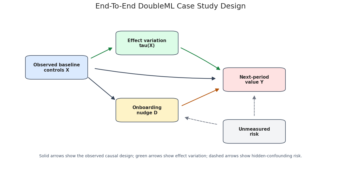
Design Diagram

The diagram below now focuses only on the causal design. The nuisance models used by DoubleML are introduced later in the estimation section. Keeping the graph causal makes the arrows easier to read: baseline controls affect both nudge assignment and future value, the nudge affects future value, baseline profile can modify the treatment effect, and dashed arrows mark unmeasured-confounding risk.

nodes = {
    "X": {"xy": (0.16, 0.66), "label": "Observed baseline\ncontrols X", "color": "#dbeafe"},
    "T": {"xy": (0.43, 0.82), "label": "Effect variation\ntau(X)", "color": "#dcfce7"},
    "D": {"xy": (0.43, 0.38), "label": "Onboarding\nnudge D", "color": "#fef3c7"},
    "Y": {"xy": (0.75, 0.58), "label": "Next-period\nvalue Y", "color": "#fee2e2"},
    "U": {"xy": (0.75, 0.24), "label": "Unmeasured\nrisk", "color": "#f3f4f6"},
}

fig, ax = plt.subplots(figsize=(12, 6.2))
ax.set_axis_off()
ax.set_xlim(0.00, 1.00)
ax.set_ylim(0.00, 1.00)
box_w, box_h = 0.15, 0.12


def anchor(node, side):
    x, y = nodes[node]["xy"]
    offsets = {
        "left": (-box_w / 2, 0),
        "right": (box_w / 2, 0),
        "top": (0, box_h / 2),
        "bottom": (0, -box_h / 2),
        "upper_right": (box_w / 2, box_h * 0.25),
        "lower_right": (box_w / 2, -box_h * 0.25),
        "upper_left": (-box_w / 2, box_h * 0.25),
        "lower_left": (-box_w / 2, -box_h * 0.25),
    }
    dx, dy = offsets[side]
    return np.array([x + dx, y + dy], dtype=float)


def shorten(start, end, gap=0.038):
    start = np.asarray(start, dtype=float)
    end = np.asarray(end, dtype=float)
    delta = end - start
    length = np.hypot(delta[0], delta[1])
    if length == 0:
        return tuple(start), tuple(end)
    unit = delta / length
    return tuple(start + gap * unit), tuple(end - gap * unit)


def draw_arrow(start, end, color="#334155", style="solid", rad=0.0, linewidth=1.7):
    start, end = shorten(start, end)
    arrow = FancyArrowPatch(
        start,
        end,
        arrowstyle="-|>",
        mutation_scale=18,
        linewidth=linewidth,
        color=color,
        linestyle=style,
        connectionstyle=f"arc3,rad={rad}",
        zorder=2,
        clip_on=False,
    )
    ax.add_patch(arrow)

# Observed causal design paths.
draw_arrow(anchor("X", "lower_right"), anchor("D", "upper_left"), color="#334155")
draw_arrow(anchor("X", "right"), anchor("Y", "left"), color="#334155", rad=0.04)
draw_arrow(anchor("D", "right"), anchor("Y", "lower_left"), color="#b45309")

# Effect-modification path: X determines who benefits more; tau(X) changes the treatment response.
draw_arrow(anchor("X", "upper_right"), anchor("T", "left"), color="#15803d")
draw_arrow(anchor("T", "right"), anchor("Y", "upper_left"), color="#15803d", rad=-0.03)

# Dashed paths show what would threaten the observed-design claim.
draw_arrow(anchor("U", "upper_left"), anchor("D", "lower_right"), color="#6b7280", style="dashed", rad=-0.02, linewidth=1.4)
draw_arrow(anchor("U", "top"), anchor("Y", "bottom"), color="#6b7280", style="dashed", linewidth=1.4)

for spec in nodes.values():
    x, y = spec["xy"]
    rect = FancyBboxPatch(
        (x - box_w / 2, y - box_h / 2),
        box_w,
        box_h,
        boxstyle="round,pad=0.018",
        facecolor=spec["color"],
        edgecolor="#334155",
        linewidth=1.2,
        zorder=3,
    )
    ax.add_patch(rect)
    ax.text(x, y, spec["label"], ha="center", va="center", fontsize=11, fontweight="bold", zorder=4)

ax.text(
    0.50,
    0.08,
    "Solid arrows show the observed causal design; green arrows show effect variation; dashed arrows show hidden-confounding risk.",
    ha="center",
    va="center",
    fontsize=10,
    color="#475569",
)
ax.set_title("End-To-End DoubleML Case Study Design", pad=18)
plt.tight_layout()
fig.savefig(FIGURE_DIR / f"{NOTEBOOK_PREFIX}_case_study_design_dag.png", dpi=160, bbox_inches="tight")
plt.show()

The dashed arrows represent residual hidden-confounding risk. DoubleML can estimate an orthogonal score for the observed design, but it cannot verify that all relevant confounders are measured.

Naive And Adjusted Baselines

Before fitting DoubleML, we compute two simple baselines. The naive difference in means ignores confounding. The adjusted linear regression controls for the same pre-treatment features but uses a simple linear outcome model. These are comparison points, not the final estimator.

treated_mean = case_df.loc[case_df["onboarding_nudge"].eq(1), "next_period_value"].mean()
control_mean = case_df.loc[case_df["onboarding_nudge"].eq(0), "next_period_value"].mean()
naive_diff = treated_mean - control_mean

ols_features = case_df[["onboarding_nudge"] + x_cols]
ols_model = LinearRegression().fit(ols_features, case_df["next_period_value"])
ols_adjusted_effect = float(ols_model.coef_[0])

baseline_estimates = pd.DataFrame(
    [
        {"estimator": "Naive difference in means", "estimate": naive_diff, "true_ate": case_df["true_treatment_effect"].mean()},
        {"estimator": "Adjusted linear regression", "estimate": ols_adjusted_effect, "true_ate": case_df["true_treatment_effect"].mean()},
    ]
)
baseline_estimates["absolute_error"] = (baseline_estimates["estimate"] - baseline_estimates["true_ate"]).abs()

save_table(baseline_estimates, f"{NOTEBOOK_PREFIX}_baseline_estimates.csv")
display(baseline_estimates)

	estimator	estimate	true_ate	absolute_error
0	Naive difference in means	0.902143	0.425708	0.476436
1	Adjusted linear regression	0.412130	0.425708	0.013578

The naive estimate is expected to be biased because treatment assignment depends on baseline intent and other features. The adjusted linear regression is a stronger baseline, but it still imposes simple functional-form assumptions.

Fit The Main DoubleML IRM Model

The main model uses DoubleMLIRM because the treatment is binary. We use random forests for both outcome nuisance functions and the propensity model. Cross-fitting ensures that the score contribution for each row uses nuisance predictions from models that did not train on that row.

main_outcome_learner = RandomForestRegressor(
    n_estimators=240,
    min_samples_leaf=12,
    max_features="sqrt",
    random_state=RANDOM_SEED,
    n_jobs=-1,
)
main_propensity_learner = RandomForestClassifier(
    n_estimators=240,
    min_samples_leaf=12,
    max_features="sqrt",
    random_state=RANDOM_SEED + 1,
    n_jobs=-1,
)

main_irm, main_row, main_predictions = fit_irm(
    case_df,
    x_cols=x_cols,
    learner_g=main_outcome_learner,
    learner_m=main_propensity_learner,
    label="Random forest IRM",
)

main_estimate = pd.DataFrame([main_row])
save_table(main_estimate, f"{NOTEBOOK_PREFIX}_main_irm_estimate.csv")
display(main_estimate)

	model	estimate	std_error	ci_95_lower	ci_95_upper	true_ate	absolute_error	ml_g0_rmse	ml_g1_rmse	ml_m_log_loss	propensity_min	propensity_p05	propensity_median	propensity_p95	propensity_max
0	Random forest IRM	0.461497	0.037944	0.387127	0.535866	0.425708	0.035789	0.980687	0.980966	0.472507	0.09138	0.208811	0.460587	0.73166	0.868944

The main DoubleML estimate should be read with its confidence interval, not only the point estimate. Because this is a simulation, we can also compare it to the true ATE. In real data, that column would be unavailable.

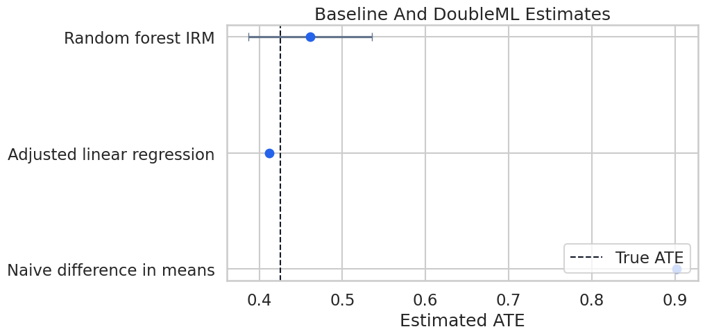
Main Estimate Plot

The next plot compares the naive baseline, adjusted linear regression, and main DoubleML estimate against the known true ATE. This is a teaching plot: in real applications, the true vertical line would be replaced by a design-based benchmark or omitted entirely.

main_plot_df = pd.concat(
    [
        baseline_estimates.rename(columns={"estimator": "model"})[["model", "estimate", "true_ate"]],
        main_estimate[["model", "estimate", "true_ate", "ci_95_lower", "ci_95_upper"]],
    ],
    ignore_index=True,
)
main_plot_df["ci_95_lower"] = main_plot_df["ci_95_lower"].fillna(main_plot_df["estimate"])
main_plot_df["ci_95_upper"] = main_plot_df["ci_95_upper"].fillna(main_plot_df["estimate"])
main_plot_df["lower_error"] = main_plot_df["estimate"] - main_plot_df["ci_95_lower"]
main_plot_df["upper_error"] = main_plot_df["ci_95_upper"] - main_plot_df["estimate"]

fig, ax = plt.subplots(figsize=(10.5, 5.2))
ax.axvline(case_df["true_treatment_effect"].mean(), color="#111827", linestyle="--", linewidth=1.5, label="True ATE")
ax.errorbar(
    x=main_plot_df["estimate"],
    y=np.arange(len(main_plot_df)),
    xerr=[main_plot_df["lower_error"], main_plot_df["upper_error"]],
    fmt="o",
    color="#2563eb",
    ecolor="#64748b",
    capsize=4,
)
ax.set_yticks(np.arange(len(main_plot_df)))
ax.set_yticklabels(main_plot_df["model"])
ax.set_xlabel("Estimated ATE")
ax.set_ylabel("")
ax.set_title("Baseline And DoubleML Estimates")
ax.legend(loc="lower right")
plt.tight_layout()
fig.savefig(FIGURE_DIR / f"{NOTEBOOK_PREFIX}_main_estimate_comparison.png", dpi=160, bbox_inches="tight")
plt.show()

The visual comparison shows why end-to-end analysis is useful. A flexible orthogonal estimator should move the answer toward the known causal target when the adjustment set is correct and overlap is reasonable.

Nuisance Diagnostics

IRM relies on outcome predictions for treated and untreated potential outcomes and a propensity prediction for treatment assignment. The diagnostics below summarize the held-out nuisance performance produced by cross-fitting.

nuisance_diagnostics = pd.DataFrame(
    [
        {"nuisance_model": "ml_g0", "target": "Outcome among untreated", "metric": "RMSE", "value": main_row["ml_g0_rmse"]},
        {"nuisance_model": "ml_g1", "target": "Outcome among treated", "metric": "RMSE", "value": main_row["ml_g1_rmse"]},
        {"nuisance_model": "ml_m", "target": "Propensity", "metric": "Log loss", "value": main_row["ml_m_log_loss"]},
    ]
)

save_table(nuisance_diagnostics, f"{NOTEBOOK_PREFIX}_main_nuisance_diagnostics.csv")
display(nuisance_diagnostics)

	nuisance_model	target	metric	value
0	ml_g0	Outcome among untreated	RMSE	0.980687
1	ml_g1	Outcome among treated	RMSE	0.980966
2	ml_m	Propensity	Log loss	0.472507

These diagnostics are numerical checks, not causal proof. Good nuisance performance supports the estimation workflow, but the identification assumptions still come from the study design.

Propensity Overlap Diagnostics

Overlap is central for binary-treatment causal inference. If estimated propensities are extremely close to zero or one, the doubly robust score can become unstable because inverse-propensity terms get large.

propensity_diagnostics = pd.DataFrame(
    [
        {"metric": "min", "value": main_predictions["propensity_hat"].min()},
        {"metric": "p01", "value": main_predictions["propensity_hat"].quantile(0.01)},
        {"metric": "p05", "value": main_predictions["propensity_hat"].quantile(0.05)},
        {"metric": "median", "value": main_predictions["propensity_hat"].median()},
        {"metric": "p95", "value": main_predictions["propensity_hat"].quantile(0.95)},
        {"metric": "p99", "value": main_predictions["propensity_hat"].quantile(0.99)},
        {"metric": "max", "value": main_predictions["propensity_hat"].max()},
        {"metric": "share_below_0.05", "value": (main_predictions["propensity_hat"] < 0.05).mean()},
        {"metric": "share_above_0.95", "value": (main_predictions["propensity_hat"] > 0.95).mean()},
    ]
)

save_table(propensity_diagnostics, f"{NOTEBOOK_PREFIX}_propensity_diagnostics.csv")
display(propensity_diagnostics)

	metric	value
0	min	0.091380
1	p01	0.157453
2	p05	0.208811
3	median	0.460587
4	p95	0.731660
5	p99	0.806554
6	max	0.868944
7	share_below_0.05	0.000000
8	share_above_0.95	0.000000

The estimated propensity distribution has no mass near the extreme boundaries after clipping. That makes the ATE estimate easier to trust numerically than a setting with many near-deterministic treatment assignments.

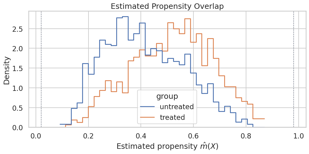
Plot Estimated Propensity Overlap

The histogram compares estimated propensity scores for treated and untreated users. We want enough overlap that both groups appear across the central support.

propensity_plot_df = case_df[["onboarding_nudge"]].join(main_predictions[["propensity_hat"]])
propensity_plot_df["group"] = np.where(propensity_plot_df["onboarding_nudge"].eq(1), "treated", "untreated")

fig, ax = plt.subplots(figsize=(10.5, 5.4))
sns.histplot(
    data=propensity_plot_df,
    x="propensity_hat",
    hue="group",
    bins=36,
    stat="density",
    common_norm=False,
    element="step",
    fill=False,
    linewidth=2,
    ax=ax,
)
ax.axvline(0.02, color="#6b7280", linestyle="--", linewidth=1, label="clipping threshold")
ax.axvline(0.98, color="#6b7280", linestyle="--", linewidth=1)
ax.set_title("Estimated Propensity Overlap")
ax.set_xlabel(r"Estimated propensity $\hat{m}(X)$")
ax.set_ylabel("Density")
plt.tight_layout()
fig.savefig(FIGURE_DIR / f"{NOTEBOOK_PREFIX}_propensity_overlap.png", dpi=160, bbox_inches="tight")
plt.show()

The treated and untreated distributions overlap in the middle of the propensity range. If one group appeared only near zero or one, the ATE would rely heavily on extrapolation.

Compare Learner Families

A complete case study should check whether the main result is a product of one learner choice. We compare three nuisance-model families: a linear/logistic baseline, random forests, and histogram gradient boosting.

learner_specs = {
    "Linear-logistic IRM": {
        "ml_g": make_pipeline(StandardScaler(), LassoCV(cv=5, random_state=RANDOM_SEED, max_iter=10_000)),
        "ml_m": make_pipeline(StandardScaler(), LogisticRegression(max_iter=2_000, solver="lbfgs")),
    },
    "Random forest IRM": {
        "ml_g": main_outcome_learner,
        "ml_m": main_propensity_learner,
    },
    "Histogram gradient boosting IRM": {
        "ml_g": HistGradientBoostingRegressor(max_iter=180, learning_rate=0.05, min_samples_leaf=25, random_state=RANDOM_SEED),
        "ml_m": HistGradientBoostingClassifier(max_iter=180, learning_rate=0.05, min_samples_leaf=25, random_state=RANDOM_SEED + 2),
    },
}

learner_rows = []
learner_models = {}
learner_predictions = {}
for label, spec in learner_specs.items():
    model, row, preds = fit_irm(
        case_df,
        x_cols=x_cols,
        learner_g=spec["ml_g"],
        learner_m=spec["ml_m"],
        label=label,
    )
    learner_models[label] = model
    learner_predictions[label] = preds
    learner_rows.append(row)

learner_comparison = pd.DataFrame(learner_rows).sort_values("absolute_error")
save_table(learner_comparison, f"{NOTEBOOK_PREFIX}_learner_family_comparison.csv")
display(learner_comparison)

	model	estimate	std_error	ci_95_lower	ci_95_upper	true_ate	absolute_error	ml_g0_rmse	ml_g1_rmse	ml_m_log_loss	propensity_min	propensity_p05	propensity_median	propensity_p95	propensity_max
0	Linear-logistic IRM	0.410063	0.034676	0.342100	0.478026	0.425708	0.015645	0.892582	0.899940	0.466185	0.042807	0.176977	0.458474	0.774297	0.958462
1	Random forest IRM	0.457877	0.037706	0.383974	0.531780	0.425708	0.032170	0.978987	0.975234	0.471871	0.084552	0.211543	0.464042	0.729396	0.885520
2	Histogram gradient boosting IRM	0.333706	0.048376	0.238891	0.428521	0.425708	0.092002	0.971182	0.959456	0.492131	0.020000	0.106707	0.454504	0.848139	0.967526

The learner comparison should be read as robustness evidence. If all reasonable learner families tell a similar story, the result is less dependent on a single modeling choice. If they diverge, the report should slow down and explain why.

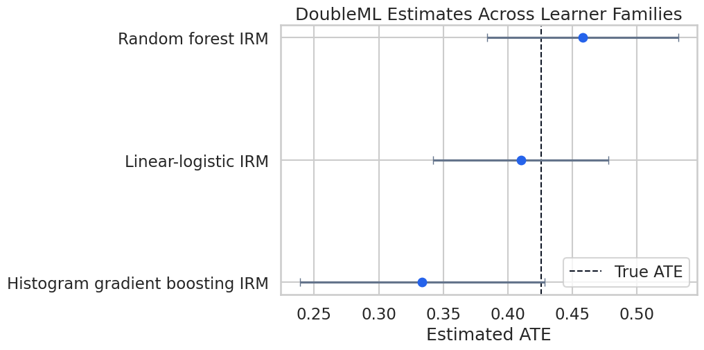
Plot Learner Family Estimates

The plot below compares point estimates and confidence intervals across nuisance learner choices. The true ATE line is available only because this is a teaching simulation.

learner_plot = learner_comparison.sort_values("estimate").copy()
learner_plot["lower_error"] = learner_plot["estimate"] - learner_plot["ci_95_lower"]
learner_plot["upper_error"] = learner_plot["ci_95_upper"] - learner_plot["estimate"]

fig, ax = plt.subplots(figsize=(10.5, 5.4))
ax.axvline(case_df["true_treatment_effect"].mean(), color="#111827", linestyle="--", linewidth=1.5, label="True ATE")
ax.errorbar(
    x=learner_plot["estimate"],
    y=np.arange(len(learner_plot)),
    xerr=[learner_plot["lower_error"], learner_plot["upper_error"]],
    fmt="o",
    color="#2563eb",
    ecolor="#64748b",
    capsize=4,
)
ax.set_yticks(np.arange(len(learner_plot)))
ax.set_yticklabels(learner_plot["model"])
ax.set_xlabel("Estimated ATE")
ax.set_ylabel("")
ax.set_title("DoubleML Estimates Across Learner Families")
ax.legend(loc="lower right")
plt.tight_layout()
fig.savefig(FIGURE_DIR / f"{NOTEBOOK_PREFIX}_learner_family_estimates.png", dpi=160, bbox_inches="tight")
plt.show()

The estimates are close enough to support a coherent main story. The learner table still belongs in the final report because it shows the result is not simply a random-forest artifact.

Doubly Robust Signal For Segment Diagnostics

The doubly robust signal is useful for exploratory subgroup summaries. Here we use it to ask whether high-intent users appear to benefit more from the nudge. This is a diagnostic use of the score signal, not a replacement for a formal policy-learning or GATE analysis.

case_df_with_signal = case_df.copy()
case_df_with_signal["dr_signal"] = doubly_robust_signal(case_df, main_predictions)

segment_summary = (
    case_df_with_signal.groupby("intent_segment", observed=True)
    .agg(
        n=("dr_signal", "size"),
        dr_ate=("dr_signal", "mean"),
        dr_se=("dr_signal", lambda x: x.std(ddof=1) / np.sqrt(len(x))),
        true_segment_ate=("true_treatment_effect", "mean"),
        treatment_rate=("onboarding_nudge", "mean"),
    )
    .reset_index()
)
segment_summary["ci_95_lower"] = segment_summary["dr_ate"] - 1.96 * segment_summary["dr_se"]
segment_summary["ci_95_upper"] = segment_summary["dr_ate"] + 1.96 * segment_summary["dr_se"]

save_table(segment_summary, f"{NOTEBOOK_PREFIX}_segment_dr_signal_summary.csv")
display(segment_summary)

	intent_segment	n	dr_ate	dr_se	true_segment_ate	treatment_rate	ci_95_lower	ci_95_upper
0	low_intent	1067	0.314353	0.072332	0.272389	0.303655	0.172582	0.456124
1	mid_intent	1066	0.508658	0.060451	0.425631	0.462477	0.390174	0.627142
2	high_intent	1067	0.560745	0.064020	0.579102	0.623243	0.435266	0.686223

The segment summary should move in the same direction as the known heterogeneous effect pattern. In real data, this would be a hypothesis-generating diagnostic unless accompanied by a formal heterogeneity design.

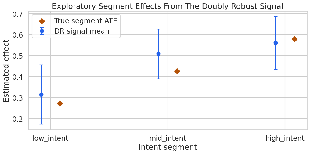
Plot Segment Effects

The segment plot compares doubly robust subgroup means with the oracle segment effects from the simulator. The oracle points are included only for teaching.

fig, ax = plt.subplots(figsize=(10.5, 5.4))
positions = np.arange(len(segment_summary))
ax.errorbar(
    positions - 0.08,
    segment_summary["dr_ate"],
    yerr=1.96 * segment_summary["dr_se"],
    fmt="o",
    color="#2563eb",
    capsize=4,
    label="DR signal mean",
)
ax.scatter(
    positions + 0.08,
    segment_summary["true_segment_ate"],
    color="#b45309",
    marker="D",
    label="True segment ATE",
)
ax.set_xticks(positions)
ax.set_xticklabels(segment_summary["intent_segment"])
ax.set_ylabel("Estimated effect")
ax.set_xlabel("Intent segment")
ax.set_title("Exploratory Segment Effects From The Doubly Robust Signal")
ax.legend(loc="upper left")
plt.tight_layout()
fig.savefig(FIGURE_DIR / f"{NOTEBOOK_PREFIX}_segment_effects.png", dpi=160, bbox_inches="tight")
plt.show()

The high-intent segment shows a larger effect, matching the way the teaching data were generated. The important reporting habit is to label this as subgroup evidence, not as an automatically deployable targeting rule.

Sample-Split Stability

Cross-fitting uses random folds. A single split can occasionally be lucky or unlucky. We refit the main random-forest specification over several deterministic fold seeds to check whether the estimate is stable.

stability_rows = []
stability_seeds = list(range(RANDOM_SEED, RANDOM_SEED + 8))

stability_outcome_learner = RandomForestRegressor(
    n_estimators=140,
    min_samples_leaf=14,
    max_features="sqrt",
    random_state=RANDOM_SEED,
    n_jobs=-1,
)
stability_propensity_learner = RandomForestClassifier(
    n_estimators=140,
    min_samples_leaf=14,
    max_features="sqrt",
    random_state=RANDOM_SEED + 1,
    n_jobs=-1,
)

for seed in stability_seeds:
    sample_splits = make_kfold_splits(len(case_df), seed=seed, n_splits=5)
    model, row, _ = fit_irm(
        case_df,
        x_cols=x_cols,
        learner_g=stability_outcome_learner,
        learner_m=stability_propensity_learner,
        label=f"split_seed_{seed}",
        sample_splits=sample_splits,
    )
    row["split_seed"] = seed
    stability_rows.append(row)

split_stability = pd.DataFrame(stability_rows)
split_stability_summary = pd.DataFrame(
    [
        {
            "n_repetitions": len(split_stability),
            "mean_estimate": split_stability["estimate"].mean(),
            "sd_estimate": split_stability["estimate"].std(ddof=1),
            "min_estimate": split_stability["estimate"].min(),
            "max_estimate": split_stability["estimate"].max(),
            "true_ate": case_df["true_treatment_effect"].mean(),
        }
    ]
)

save_table(split_stability, f"{NOTEBOOK_PREFIX}_sample_split_stability.csv")
save_table(split_stability_summary, f"{NOTEBOOK_PREFIX}_sample_split_stability_summary.csv")
display(split_stability_summary)

	n_repetitions	mean_estimate	sd_estimate	min_estimate	max_estimate	true_ate
0	8	0.462021	0.006578	0.450427	0.469819	0.425708

The repeated-split standard deviation is a practical stability check. If fold randomness changed the conclusion, the final report would need to say so and rely on repeated cross-fitting or a more stable design.

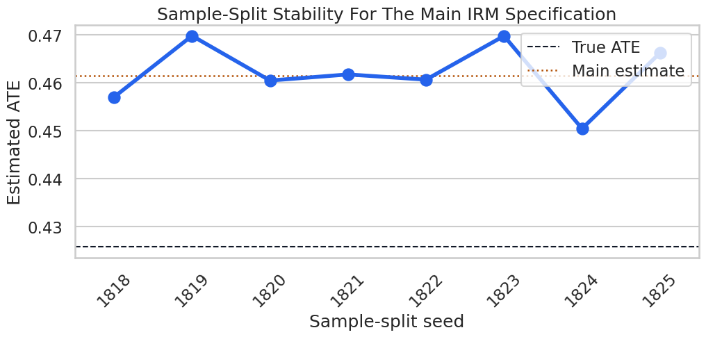
Plot Sample-Split Stability

This plot shows the repeated estimates against the main estimate and true ATE. It is a compact way to communicate whether cross-fitting randomness matters materially.

fig, ax = plt.subplots(figsize=(10.5, 5.2))
ax.axhline(case_df["true_treatment_effect"].mean(), color="#111827", linestyle="--", linewidth=1.5, label="True ATE")
ax.axhline(main_row["estimate"], color="#b45309", linestyle=":", linewidth=1.8, label="Main estimate")
sns.pointplot(
    data=split_stability,
    x="split_seed",
    y="estimate",
    color="#2563eb",
    errorbar=None,
    ax=ax,
)
ax.set_title("Sample-Split Stability For The Main IRM Specification")
ax.set_xlabel("Sample-split seed")
ax.set_ylabel("Estimated ATE")
ax.tick_params(axis="x", rotation=45)
ax.legend(loc="upper right")
plt.tight_layout()
fig.savefig(FIGURE_DIR / f"{NOTEBOOK_PREFIX}_sample_split_stability.png", dpi=160, bbox_inches="tight")
plt.show()

The repeated estimates cluster around the same value. This supports the numerical stability of the main estimate under alternative fold assignments.

Sensitivity Analysis For Hidden Confounding

The final statistical check uses DoubleML’s sensitivity analysis. The parameters cf_y and cf_d describe the strength of an unobserved confounder in the outcome and treatment equations. The parameter rho controls the direction of confounding. These are not discovered from the data; they are stress-test settings.

def extract_sensitivity_row(model, scenario, cf_y, cf_d, rho):
    params = model.sensitivity_params
    return {
        "scenario": scenario,
        "cf_y": cf_y,
        "cf_d": cf_d,
        "rho": rho,
        "theta_lower": float(params["theta"]["lower"][0]),
        "theta": float(model.coef[0]),
        "theta_upper": float(params["theta"]["upper"][0]),
        "ci_lower": float(params["ci"]["lower"][0]),
        "ci_upper": float(params["ci"]["upper"][0]),
        "rv_percent": float(params["rv"][0] * 100),
        "rva_percent": float(params["rva"][0] * 100),
    }

sensitivity_specs = [
    ("mild", 0.01, 0.01, 1.0),
    ("moderate", 0.03, 0.03, 1.0),
    ("strong", 0.06, 0.06, 1.0),
]

sensitivity_rows = []
for scenario, cf_y, cf_d, rho in sensitivity_specs:
    main_irm.sensitivity_analysis(cf_y=cf_y, cf_d=cf_d, rho=rho, level=0.95, null_hypothesis=0.0)
    sensitivity_rows.append(extract_sensitivity_row(main_irm, scenario, cf_y, cf_d, rho))

sensitivity_summary = pd.DataFrame(sensitivity_rows)
save_table(sensitivity_summary, f"{NOTEBOOK_PREFIX}_sensitivity_summary.csv")
display(sensitivity_summary)

# Restore the moderate scenario as the active sensitivity setting for anyone inspecting the model object later.
main_irm.sensitivity_analysis(cf_y=0.03, cf_d=0.03, rho=1.0, level=0.95, null_hypothesis=0.0)

	scenario	cf_y	cf_d	rho	theta_lower	theta	theta_upper	ci_lower	ci_upper	rv_percent	rva_percent
0	mild	0.01	0.01	1.0	0.440392	0.461497	0.482602	0.377922	0.544962	19.694041	17.213465
1	moderate	0.03	0.03	1.0	0.397532	0.461497	0.525462	0.334932	0.587729	19.694041	17.213465
2	strong	0.06	0.06	1.0	0.331541	0.461497	0.591453	0.268705	0.653612	19.694041	17.213465

<doubleml.irm.irm.DoubleMLIRM at 0x78c3c2bb5fd0>

The sensitivity table asks how much the estimate could move under increasingly strong hidden-confounding scenarios. It does not prove that hidden confounding is absent. It makes the remaining assumption visible.

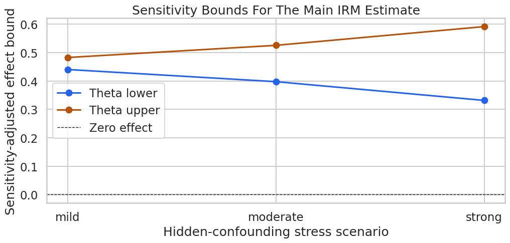
Plot Sensitivity Bounds

The sensitivity plot shows how the lower and upper treatment-effect bounds change as the hidden-confounding stress test gets stronger.

fig, ax = plt.subplots(figsize=(10.5, 5.2))
positions = np.arange(len(sensitivity_summary))
ax.plot(positions, sensitivity_summary["theta_lower"], marker="o", color="#2563eb", label="Theta lower")
ax.plot(positions, sensitivity_summary["theta_upper"], marker="o", color="#b45309", label="Theta upper")
ax.axhline(0, color="#111827", linestyle="--", linewidth=1, label="Zero effect")
ax.set_xticks(positions)
ax.set_xticklabels(sensitivity_summary["scenario"])
ax.set_ylabel("Sensitivity-adjusted effect bound")
ax.set_xlabel("Hidden-confounding stress scenario")
ax.set_title("Sensitivity Bounds For The Main IRM Estimate")
ax.legend(loc="best")
plt.tight_layout()
fig.savefig(FIGURE_DIR / f"{NOTEBOOK_PREFIX}_sensitivity_bounds.png", dpi=160, bbox_inches="tight")
plt.show()

The sensitivity bounds communicate the main limitation of observational analysis: the result can be numerically precise and still depend on an untestable adjustment assumption.

Final Evidence Scorecard

The scorecard pulls together the pieces a reviewer should see before trusting the result. It includes design, overlap, nuisance quality, learner robustness, split stability, heterogeneity, and sensitivity.

evidence_scorecard = pd.DataFrame(
    [
        {
            "evidence_area": "Design",
            "finding": "Only pre-treatment controls are used in the main feature set.",
            "status": "documented",
        },
        {
            "evidence_area": "Main estimate",
            "finding": f"Main IRM ATE is {main_row['estimate']:.3f} with 95% CI [{main_row['ci_95_lower']:.3f}, {main_row['ci_95_upper']:.3f}].",
            "status": "estimated",
        },
        {
            "evidence_area": "Overlap",
            "finding": f"Estimated propensity p05={main_row['propensity_p05']:.3f}, p95={main_row['propensity_p95']:.3f}.",
            "status": "checked",
        },
        {
            "evidence_area": "Learner robustness",
            "finding": f"Learner-family estimates range from {learner_comparison['estimate'].min():.3f} to {learner_comparison['estimate'].max():.3f}.",
            "status": "checked",
        },
        {
            "evidence_area": "Sample splitting",
            "finding": f"Repeated split SD is {split_stability_summary.loc[0, 'sd_estimate']:.4f}.",
            "status": "checked",
        },
        {
            "evidence_area": "Heterogeneity",
            "finding": "DR signal summaries suggest larger effects for higher-intent users.",
            "status": "exploratory",
        },
        {
            "evidence_area": "Sensitivity",
            "finding": "Sensitivity bounds are reported for mild, moderate, and strong hidden-confounding scenarios.",
            "status": "stress tested",
        },
        {
            "evidence_area": "Limitations",
            "finding": "Unmeasured confounding, measurement error, and deployment interference remain design risks.",
            "status": "must report",
        },
    ]
)

save_table(evidence_scorecard, f"{NOTEBOOK_PREFIX}_evidence_scorecard.csv")
display(evidence_scorecard)

	evidence_area	finding	status
0	Design	Only pre-treatment controls are used in the ma...	documented
1	Main estimate	Main IRM ATE is 0.461 with 95% CI [0.387, 0.536].	estimated
2	Overlap	Estimated propensity p05=0.209, p95=0.732.	checked
3	Learner robustness	Learner-family estimates range from 0.334 to 0...	checked
4	Sample splitting	Repeated split SD is 0.0066.	checked
5	Heterogeneity	DR signal summaries suggest larger effects for...	exploratory
6	Sensitivity	Sensitivity bounds are reported for mild, mode...	stress tested
7	Limitations	Unmeasured confounding, measurement error, and...	must report

The scorecard is a compact review object. It is the bridge between a technical notebook and a reader who wants to know whether the analysis is credible.

Write The Final Case Study Report

The report template below is written as if this were the final deliverable. It includes the causal question, estimator, main estimate, diagnostics, sensitivity, subgroup findings, and limitations.

report_text = rf"""# End-To-End DoubleML Case Study Report

## Causal Question
Estimate the average effect of receiving a guided onboarding nudge on next-period user value.

## Estimand
The target estimand is the average treatment effect:

$$
\theta_0 = \mathbb{{E}}[Y(1) - Y(0)].
$$

## Identification Assumptions
The analysis assumes conditional exchangeability given the documented pre-treatment controls, overlap between treated and untreated users, stable treatment definition, and no interference across users.

## Main DoubleML Specification
- Estimator: `DoubleMLIRM`
- Score: ATE
- Outcome learner: random forest regressor
- Propensity learner: random forest classifier
- Cross-fitting: 5 folds
- Propensity clipping threshold: 0.02

## Main Estimate
- Estimated ATE: {main_row['estimate']:.4f}
- Standard error: {main_row['std_error']:.4f}
- 95% confidence interval: [{main_row['ci_95_lower']:.4f}, {main_row['ci_95_upper']:.4f}]
- Known true ATE in this teaching simulation: {main_row['true_ate']:.4f}

## Diagnostics
- Estimated propensity p05 / p95: {main_row['propensity_p05']:.4f} / {main_row['propensity_p95']:.4f}
- Outcome RMSE under control model: {main_row['ml_g0_rmse']:.4f}
- Outcome RMSE under treated model: {main_row['ml_g1_rmse']:.4f}
- Propensity log loss: {main_row['ml_m_log_loss']:.4f}
- Sample-split estimate SD: {split_stability_summary.loc[0, 'sd_estimate']:.4f}

## Heterogeneity
The doubly robust signal suggests larger effects for higher-intent users. Treat this as subgroup evidence, not as a fully validated targeting policy.

## Sensitivity
Sensitivity bounds are saved for mild, moderate, and strong hidden-confounding scenarios. These stress tests do not remove hidden-confounding risk; they describe how the estimate would move under specified scenarios.

## Limitations
The analysis remains observational. It can be threatened by missing confounders, bad measurement, outcome leakage, violations of overlap, interference, or changes in the treatment definition.

## Artifact Paths
- Data: `{DATASET_DIR / f'{NOTEBOOK_PREFIX}_end_to_end_case_study_data.csv'}`
- Main estimate: `{TABLE_DIR / f'{NOTEBOOK_PREFIX}_main_irm_estimate.csv'}`
- Learner comparison: `{TABLE_DIR / f'{NOTEBOOK_PREFIX}_learner_family_comparison.csv'}`
- Segment summary: `{TABLE_DIR / f'{NOTEBOOK_PREFIX}_segment_dr_signal_summary.csv'}`
- Sensitivity summary: `{TABLE_DIR / f'{NOTEBOOK_PREFIX}_sensitivity_summary.csv'}`
- Evidence scorecard: `{TABLE_DIR / f'{NOTEBOOK_PREFIX}_evidence_scorecard.csv'}`
"""

report_path = REPORT_DIR / f"{NOTEBOOK_PREFIX}_end_to_end_case_study_report.md"
report_path.write_text(report_text)
print(f"Wrote report to: {report_path}")

Wrote report to: /home/apex/Documents/ranking_sys/notebooks/tutorials/doubleml/outputs/reports/18_end_to_end_case_study_report.md

The report is short on purpose. A final case-study report should not reproduce every notebook cell. It should tell a clear story and point to the artifacts that support that story.

Artifact Manifest

The final manifest lists every major output from this notebook. This makes the case study easy to review outside the notebook interface.

artifact_manifest = pd.DataFrame(
    [
        {"artifact": "Case study dataset", "path": str(DATASET_DIR / f"{NOTEBOOK_PREFIX}_end_to_end_case_study_data.csv")},
        {"artifact": "Roadmap", "path": str(TABLE_DIR / f"{NOTEBOOK_PREFIX}_case_study_roadmap.csv")},
        {"artifact": "Field dictionary", "path": str(TABLE_DIR / f"{NOTEBOOK_PREFIX}_field_dictionary.csv")},
        {"artifact": "Data audit", "path": str(TABLE_DIR / f"{NOTEBOOK_PREFIX}_data_audit.csv")},
        {"artifact": "Baseline estimates", "path": str(TABLE_DIR / f"{NOTEBOOK_PREFIX}_baseline_estimates.csv")},
        {"artifact": "Main IRM estimate", "path": str(TABLE_DIR / f"{NOTEBOOK_PREFIX}_main_irm_estimate.csv")},
        {"artifact": "Nuisance diagnostics", "path": str(TABLE_DIR / f"{NOTEBOOK_PREFIX}_main_nuisance_diagnostics.csv")},
        {"artifact": "Propensity diagnostics", "path": str(TABLE_DIR / f"{NOTEBOOK_PREFIX}_propensity_diagnostics.csv")},
        {"artifact": "Learner family comparison", "path": str(TABLE_DIR / f"{NOTEBOOK_PREFIX}_learner_family_comparison.csv")},
        {"artifact": "Segment DR signal summary", "path": str(TABLE_DIR / f"{NOTEBOOK_PREFIX}_segment_dr_signal_summary.csv")},
        {"artifact": "Sample split stability", "path": str(TABLE_DIR / f"{NOTEBOOK_PREFIX}_sample_split_stability.csv")},
        {"artifact": "Sensitivity summary", "path": str(TABLE_DIR / f"{NOTEBOOK_PREFIX}_sensitivity_summary.csv")},
        {"artifact": "Evidence scorecard", "path": str(TABLE_DIR / f"{NOTEBOOK_PREFIX}_evidence_scorecard.csv")},
        {"artifact": "Design DAG", "path": str(FIGURE_DIR / f"{NOTEBOOK_PREFIX}_case_study_design_dag.png")},
        {"artifact": "Main estimate comparison", "path": str(FIGURE_DIR / f"{NOTEBOOK_PREFIX}_main_estimate_comparison.png")},
        {"artifact": "Propensity overlap", "path": str(FIGURE_DIR / f"{NOTEBOOK_PREFIX}_propensity_overlap.png")},
        {"artifact": "Learner estimates", "path": str(FIGURE_DIR / f"{NOTEBOOK_PREFIX}_learner_family_estimates.png")},
        {"artifact": "Segment effects", "path": str(FIGURE_DIR / f"{NOTEBOOK_PREFIX}_segment_effects.png")},
        {"artifact": "Sample split stability figure", "path": str(FIGURE_DIR / f"{NOTEBOOK_PREFIX}_sample_split_stability.png")},
        {"artifact": "Sensitivity bounds", "path": str(FIGURE_DIR / f"{NOTEBOOK_PREFIX}_sensitivity_bounds.png")},
        {"artifact": "Final report", "path": str(REPORT_DIR / f"{NOTEBOOK_PREFIX}_end_to_end_case_study_report.md")},
    ]
)

save_table(artifact_manifest, f"{NOTEBOOK_PREFIX}_artifact_manifest.csv")
display(artifact_manifest)

	artifact	path
0	Case study dataset	/home/apex/Documents/ranking_sys/notebooks/tut...
1	Roadmap	/home/apex/Documents/ranking_sys/notebooks/tut...
2	Field dictionary	/home/apex/Documents/ranking_sys/notebooks/tut...
3	Data audit	/home/apex/Documents/ranking_sys/notebooks/tut...
4	Baseline estimates	/home/apex/Documents/ranking_sys/notebooks/tut...
5	Main IRM estimate	/home/apex/Documents/ranking_sys/notebooks/tut...
6	Nuisance diagnostics	/home/apex/Documents/ranking_sys/notebooks/tut...
7	Propensity diagnostics	/home/apex/Documents/ranking_sys/notebooks/tut...
8	Learner family comparison	/home/apex/Documents/ranking_sys/notebooks/tut...
9	Segment DR signal summary	/home/apex/Documents/ranking_sys/notebooks/tut...
10	Sample split stability	/home/apex/Documents/ranking_sys/notebooks/tut...
11	Sensitivity summary	/home/apex/Documents/ranking_sys/notebooks/tut...
12	Evidence scorecard	/home/apex/Documents/ranking_sys/notebooks/tut...
13	Design DAG	/home/apex/Documents/ranking_sys/notebooks/tut...
14	Main estimate comparison	/home/apex/Documents/ranking_sys/notebooks/tut...
15	Propensity overlap	/home/apex/Documents/ranking_sys/notebooks/tut...
16	Learner estimates	/home/apex/Documents/ranking_sys/notebooks/tut...
17	Segment effects	/home/apex/Documents/ranking_sys/notebooks/tut...
18	Sample split stability figure	/home/apex/Documents/ranking_sys/notebooks/tut...
19	Sensitivity bounds	/home/apex/Documents/ranking_sys/notebooks/tut...
20	Final report	/home/apex/Documents/ranking_sys/notebooks/tut...

The manifest is the table of contents for the case study outputs. It also makes the notebook easier to grade, review, or convert into a portfolio writeup.

Tutorial Wrap-Up

This case study pulls the DoubleML tutorial series together. The workflow is intentionally repeatable:

• Define the causal question and target estimand.
• Document variable timing and exclude invalid controls.
• Choose the DoubleML class that matches the treatment and data structure.
• Fit flexible nuisance models with cross-fitting.
• Report uncertainty, overlap, nuisance diagnostics, learner robustness, and split stability.
• Treat subgroup findings as exploratory unless the heterogeneity design is formal.
• Use sensitivity analysis to describe, not erase, hidden-confounding risk.
• End with a concise report and reviewable artifacts.

The main lesson is that DoubleML is a disciplined estimation framework. The quality of the answer still depends on the quality of the causal design.