DoubleML Tutorial 16: Custom Scores And Advanced API

This notebook teaches the part of DoubleML that sits closest to the estimating equation. Earlier notebooks used built-in model classes and built-in scores. That is the right default. Most practical causal projects should first try the standard classes, diagnose them well, and only then reach for custom score functions.

A custom score becomes useful when you can state a causal estimand through a Neyman-orthogonal moment condition that DoubleML does not already expose directly. In DoubleML’s linear-score classes, each observation contributes a score of the form:

\[ \psi(W_i; \theta, \eta) = \psi_a(W_i; \eta)\,\theta + \psi_b(W_i; \eta), \]

where \(W_i\) is the observed row, \(\theta\) is the causal target, and \(\eta\) collects the nuisance functions estimated by machine learning. DoubleML solves the empirical moment condition:

\[ \frac{1}{n}\sum_{i=1}^{n} \left[\psi_a(W_i; \hat{\eta})\,\theta + \psi_b(W_i; \hat{\eta})\right] = 0. \]

For a linear score, this means the coefficient can be reconstructed directly from the stored score pieces:

\[ \hat{\theta} = -\frac{\frac{1}{n}\sum_{i=1}^{n}\psi_b(W_i; \hat{\eta})} {\frac{1}{n}\sum_{i=1}^{n}\psi_a(W_i; \hat{\eta})}. \]

The key phrase is Neyman-orthogonal. Informally, orthogonality means that small first-stage nuisance-model errors do not create first-order bias in the final causal estimate. A compact way to write this condition is:

\[ \left. \frac{\partial}{\partial r} \mathbb{E}\left[\psi\left(W; \theta_0, \eta_0 + r(\eta - \eta_0)\right)\right] \right|_{r=0} = 0. \]

That condition is the reason DoubleML can combine flexible machine learning with valid causal inference. If we write a custom score that is not orthogonal, cross-fitting alone does not rescue the causal claim.

This notebook covers four advanced workflows:

• Reading and reconstructing DoubleML score elements.
• Writing an equivalent callable score for PLR.
• Writing a priority-weighted callable score.
• Using advanced APIs: custom sample splits, external nuisance predictions, stored fold models, and score diagnostics.

Setup

This setup cell prepares the shared tutorial output folders and imports the libraries used throughout the notebook. The warning filters are intentionally narrow. They remove notebook-environment noise and the expected DoubleML warning that sensitivity analysis is not implemented for callable scores in this installed version.

from pathlib import Path
import os
import warnings

# Find the repository root from wherever the notebook is executed.
PROJECT_ROOT = Path.cwd().resolve()
while not (PROJECT_ROOT / "pyproject.toml").exists() and PROJECT_ROOT != PROJECT_ROOT.parent:
    PROJECT_ROOT = PROJECT_ROOT.parent

OUTPUT_DIR = PROJECT_ROOT / "notebooks" / "tutorials" / "doubleml" / "outputs"
DATASET_DIR = OUTPUT_DIR / "datasets"
FIGURE_DIR = OUTPUT_DIR / "figures"
TABLE_DIR = OUTPUT_DIR / "tables"
REPORT_DIR = OUTPUT_DIR / "reports"
MATPLOTLIB_CACHE_DIR = OUTPUT_DIR / "matplotlib_cache"

for directory in [DATASET_DIR, FIGURE_DIR, TABLE_DIR, REPORT_DIR, MATPLOTLIB_CACHE_DIR]:
    directory.mkdir(parents=True, exist_ok=True)

# Set Matplotlib's cache before importing pyplot so notebook execution stays quiet.
os.environ.setdefault("MPLCONFIGDIR", str(MATPLOTLIB_CACHE_DIR))

warnings.filterwarnings("ignore", category=FutureWarning)
warnings.filterwarnings("ignore", message="IProgress not found.*")
warnings.filterwarnings("ignore", message="X does not have valid feature names.*")
warnings.filterwarnings("ignore", message="Sensitivity analysis not implemented for callable scores.*")

import numpy as np
import pandas as pd
import matplotlib.pyplot as plt
import seaborn as sns

from IPython.display import display
from matplotlib.patches import FancyArrowPatch, FancyBboxPatch
from sklearn.base import clone
from sklearn.ensemble import RandomForestRegressor
from sklearn.metrics import mean_absolute_error, mean_squared_error
from sklearn.model_selection import KFold

import doubleml as dml
from doubleml import DoubleMLData, DoubleMLPLR

NOTEBOOK_PREFIX = "16"
RANDOM_SEED = 160
TRUE_THETA = 1.25

sns.set_theme(style="whitegrid", context="talk")
pd.set_option("display.max_columns", 80)
pd.set_option("display.float_format", "{:.4f}".format)

print(f"Project root: {PROJECT_ROOT}")
print(f"DoubleML version: {dml.__version__}")
print(f"Outputs will be written to: {OUTPUT_DIR}")

Project root: /home/apex/Documents/ranking_sys
DoubleML version: 0.11.2
Outputs will be written to: /home/apex/Documents/ranking_sys/notebooks/tutorials/doubleml/outputs

The setup confirms the local DoubleML version and output location. Every artifact created by this notebook uses prefix 16.

Helper Functions

The helper functions below keep the notebook focused on score logic. The most important helper is fit_plr(), which lets us reuse the same sample split across built-in and callable scores. Without a shared split, two estimates can differ simply because the nuisance models were trained on different folds.

def save_table(df, filename):
    path = TABLE_DIR / filename
    df.to_csv(path, index=False)
    return df


def save_dataset(df, filename):
    path = DATASET_DIR / filename
    df.to_csv(path, index=False)
    return df


def rmse(y_true, y_pred):
    return float(np.sqrt(mean_squared_error(y_true, y_pred)))


def normalize_weights(weights):
    weights = np.asarray(weights, dtype=float)
    if weights.mean() <= 0:
        raise ValueError("Weights must have positive mean.")
    return weights / weights.mean()


def solve_linear_score(psi_a, psi_b):
    psi_a = np.asarray(psi_a, dtype=float).reshape(-1)
    psi_b = np.asarray(psi_b, dtype=float).reshape(-1)
    return float(-np.nanmean(psi_b) / np.nanmean(psi_a))


def make_plr_data(frame, x_cols):
    return DoubleMLData(frame, y_col="outcome", d_cols="treatment", x_cols=x_cols)


def fit_plr(frame, x_cols, learner_l, learner_m, score, sample_splits, store_models=False, external_predictions=None):
    dml_data = make_plr_data(frame, x_cols)
    model = DoubleMLPLR(
        dml_data,
        ml_l=clone(learner_l),
        ml_m=clone(learner_m),
        n_folds=len(sample_splits),
        score=score,
        draw_sample_splitting=False,
    )
    model.set_sample_splitting(sample_splits)
    model.fit(store_predictions=True, store_models=store_models, external_predictions=external_predictions)
    return model


def extract_plr_row(label, model, true_theta=TRUE_THETA):
    ci = model.confint()
    return {
        "model": label,
        "estimate": float(model.coef[0]),
        "std_error": float(model.se[0]),
        "ci_95_lower": float(ci.iloc[0, 0]),
        "ci_95_upper": float(ci.iloc[0, 1]),
        "true_theta": true_theta,
        "absolute_error": abs(float(model.coef[0]) - true_theta),
    }


def manual_cross_fit_predictions(frame, x_cols, sample_splits, learner_l, learner_m):
    x = frame[x_cols].to_numpy()
    y = frame["outcome"].to_numpy()
    d = frame["treatment"].to_numpy()
    l_hat = np.full(len(frame), np.nan)
    m_hat = np.full(len(frame), np.nan)

    for train_index, test_index in sample_splits:
        l_model = clone(learner_l)
        m_model = clone(learner_m)
        l_model.fit(x[train_index], y[train_index])
        m_model.fit(x[train_index], d[train_index])
        l_hat[test_index] = l_model.predict(x[test_index])
        m_hat[test_index] = m_model.predict(x[test_index])

    return l_hat, m_hat

These helpers make two advanced ideas explicit: the coefficient comes from psi_a and psi_b, and external nuisance predictions must respect the same row order as the original data.

Advanced API Vocabulary

The table below names the DoubleML features used in this notebook. These are extension tools, not replacements for identification work.

advanced_api_vocabulary = pd.DataFrame(
    [
        {
            "concept": "Linear score elements",
            "meaning": "DoubleML stores score pieces psi_a and psi_b for linear scores.",
            "why_it_matters": "They allow direct inspection of the estimating equation.",
        },
        {
            "concept": "Callable score",
            "meaning": "A user-supplied function that returns psi_a and psi_b.",
            "why_it_matters": "Useful for valid custom moments when built-in scores are not enough.",
        },
        {
            "concept": "set_sample_splitting()",
            "meaning": "A method for passing analyst-defined train/test folds.",
            "why_it_matters": "Needed for reproducible comparisons, grouped splits, or temporal splits.",
        },
        {
            "concept": "external_predictions",
            "meaning": "A nested dictionary of user-supplied nuisance predictions.",
            "why_it_matters": "Lets teams use external ML pipelines while still using DoubleML for score estimation.",
        },
        {
            "concept": "store_models=True",
            "meaning": "Stores fitted fold-level nuisance models.",
            "why_it_matters": "Useful for auditing model behavior such as feature importance.",
        },
        {
            "concept": "evaluate_learners()",
            "meaning": "Reports out-of-fold nuisance losses.",
            "why_it_matters": "A model-quality diagnostic before trusting score-based estimates.",
        },
    ]
)

save_table(advanced_api_vocabulary, f"{NOTEBOOK_PREFIX}_advanced_api_vocabulary.csv")
display(advanced_api_vocabulary)

	concept	meaning	why_it_matters
0	Linear score elements	DoubleML stores score pieces psi_a and psi_b f...	They allow direct inspection of the estimating...
1	Callable score	A user-supplied function that returns psi_a an...	Useful for valid custom moments when built-in ...
2	set_sample_splitting()	A method for passing analyst-defined train/tes...	Needed for reproducible comparisons, grouped s...
3	external_predictions	A nested dictionary of user-supplied nuisance ...	Lets teams use external ML pipelines while sti...
4	store_models=True	Stores fitted fold-level nuisance models.	Useful for auditing model behavior such as fea...
5	evaluate_learners()	Reports out-of-fold nuisance losses.	A model-quality diagnostic before trusting sco...

The vocabulary table separates score customization from pipeline customization. Custom scores change the estimating equation; external predictions and stored models change how nuisance functions are supplied or audited.

Synthetic PLR Design

We use a partially linear regression design with known constant treatment effect. The data-generating process is:

\[ Y_i = \theta_0 D_i + g_0(X_i) + \varepsilon_i, \]

\[ D_i = m_0(X_i) + V_i, \]

with \(\theta_0 = 1.25\), \(\mathbb{E}[V_i \mid X_i] = 0\), and outcome noise generated independently of the treatment residual. The nuisance functions are:

\[ g_0(X_i) = \mathbb{E}[Y_i - \theta_0 D_i \mid X_i], \qquad m_0(X_i) = \mathbb{E}[D_i \mid X_i]. \]

The true effect is TRUE_THETA = 1.25. Because the true effect is constant, the custom weighted score below should still target the same causal parameter. This makes the notebook a clean API tutorial: if estimates differ meaningfully, we can attribute the difference to score construction, nuisance quality, or finite-sample noise rather than a genuinely different heterogeneous target.

rng = np.random.default_rng(RANDOM_SEED)
n_obs = 900
n_features = 8
x_cols = [f"x{i:02d}" for i in range(n_features)]

plr_df = pd.DataFrame(rng.normal(size=(n_obs, n_features)), columns=x_cols)
plr_df["priority_score"] = 0.80 * plr_df["x00"] - 0.50 * plr_df["x01"] + 0.30 * plr_df["x02"]
plr_df["priority_segment"] = np.where(
    plr_df["priority_score"] > plr_df["priority_score"].quantile(0.70),
    "high_priority",
    "standard",
)

plr_df["true_m"] = (
    0.60 * np.sin(plr_df["x00"])
    + 0.35 * plr_df["x01"] ** 2
    - 0.30 * plr_df["x02"]
    + 0.20 * plr_df["x03"] * plr_df["x04"]
)
plr_df["true_g"] = (
    0.80 * np.cos(plr_df["x00"])
    + 0.40 * plr_df["x05"] * plr_df["x06"]
    - 0.20 * plr_df["x07"] ** 2
    + 0.25 * plr_df["x01"]
)
plr_df["treatment"] = plr_df["true_m"] + rng.normal(scale=1.00, size=n_obs)
plr_df["outcome"] = TRUE_THETA * plr_df["treatment"] + plr_df["true_g"] + rng.normal(scale=1.00, size=n_obs)

save_dataset(plr_df, f"{NOTEBOOK_PREFIX}_synthetic_custom_score_plr_data.csv")
display(plr_df.head())

	x00	x01	x02	x03	x04	x05	x06	x07	priority_score	priority_segment	true_m	true_g	treatment	outcome
0	-1.3750	0.3951	-0.9502	0.1802	-0.1471	-2.2888	1.6052	-0.1582	-1.5826	standard	-0.2541	-1.2201	-1.3374	-1.6131
1	0.7881	0.3697	0.6213	-0.1373	0.1399	0.1034	0.5752	1.0415	0.6320	high_priority	0.2830	0.4634	1.6365	3.1925
2	1.6718	1.5878	-0.9541	1.2347	-0.3838	1.5186	0.5062	-0.6749	0.2573	standard	1.6708	0.5327	2.3433	2.5286
3	1.8800	0.3869	-0.1683	0.9678	1.4453	0.0364	0.0006	1.0791	1.2600	high_priority	0.9542	-0.3796	0.0256	-1.0905
4	-0.7793	-1.5007	-0.9743	-1.3892	-0.3784	-0.2549	0.0005	-0.2917	-0.1654	standard	0.7640	0.1769	1.2301	2.8375

The first rows show observed controls, oracle nuisance functions, treatment, outcome, and a priority segment. DoubleML will not use true_m or true_g; they are present only for diagnostics.

Field Dictionary

This field dictionary documents the role of every column. It is especially important in advanced API tutorials because external predictions and custom score closures can accidentally use columns that should not enter the estimator.

field_dictionary = pd.DataFrame(
    [
        {"column": "x00-x07", "role": "Observed controls", "description": "Pre-treatment covariates used by nuisance learners."},
        {"column": "priority_score", "role": "Pre-treatment priority signal", "description": "Used to define priority weights for a custom score example."},
        {"column": "priority_segment", "role": "Reporting group", "description": "High-priority vs standard group based on priority_score."},
        {"column": "true_m", "role": "Oracle diagnostic", "description": "True treatment nuisance E[D|X]; unavailable in real data."},
        {"column": "true_g", "role": "Oracle diagnostic", "description": "True baseline outcome nuisance g0(X); unavailable in real data."},
        {"column": "treatment", "role": "Treatment", "description": "Continuous treatment variable D."},
        {"column": "outcome", "role": "Outcome", "description": "Observed continuous outcome Y."},
    ]
)

save_table(field_dictionary, f"{NOTEBOOK_PREFIX}_field_dictionary.csv")
display(field_dictionary)

	column	role	description
0	x00-x07	Observed controls	Pre-treatment covariates used by nuisance lear...
1	priority_score	Pre-treatment priority signal	Used to define priority weights for a custom s...
2	priority_segment	Reporting group	High-priority vs standard group based on prior...
3	true_m	Oracle diagnostic	True treatment nuisance E[D|X]; unavailable in...
4	true_g	Oracle diagnostic	True baseline outcome nuisance g0(X); unavaila...
5	treatment	Treatment	Continuous treatment variable D.
6	outcome	Outcome	Observed continuous outcome Y.

The priority variables are pre-treatment signals. That matters because custom weighting based on post-treatment variables would change the causal question and usually break identification.

Data Audit

The audit below checks sample size, treatment scale, outcome scale, priority-group size, and the true causal effect.

data_audit = pd.DataFrame(
    [
        {"metric": "rows", "value": len(plr_df)},
        {"metric": "true_theta", "value": TRUE_THETA},
        {"metric": "treatment_mean", "value": plr_df["treatment"].mean()},
        {"metric": "treatment_std", "value": plr_df["treatment"].std()},
        {"metric": "outcome_mean", "value": plr_df["outcome"].mean()},
        {"metric": "outcome_std", "value": plr_df["outcome"].std()},
        {"metric": "high_priority_share", "value": plr_df["priority_segment"].eq("high_priority").mean()},
    ]
)

save_table(data_audit, f"{NOTEBOOK_PREFIX}_data_audit.csv")
display(data_audit)

	metric	value
0	rows	900.0000
1	true_theta	1.2500
2	treatment_mean	0.3563
3	treatment_std	1.2197
4	outcome_mean	0.8018
5	outcome_std	1.9793
6	high_priority_share	0.3000

The high-priority segment is about 30% of the data by construction. That gives enough rows for the weighted-score example without making the target population too small.

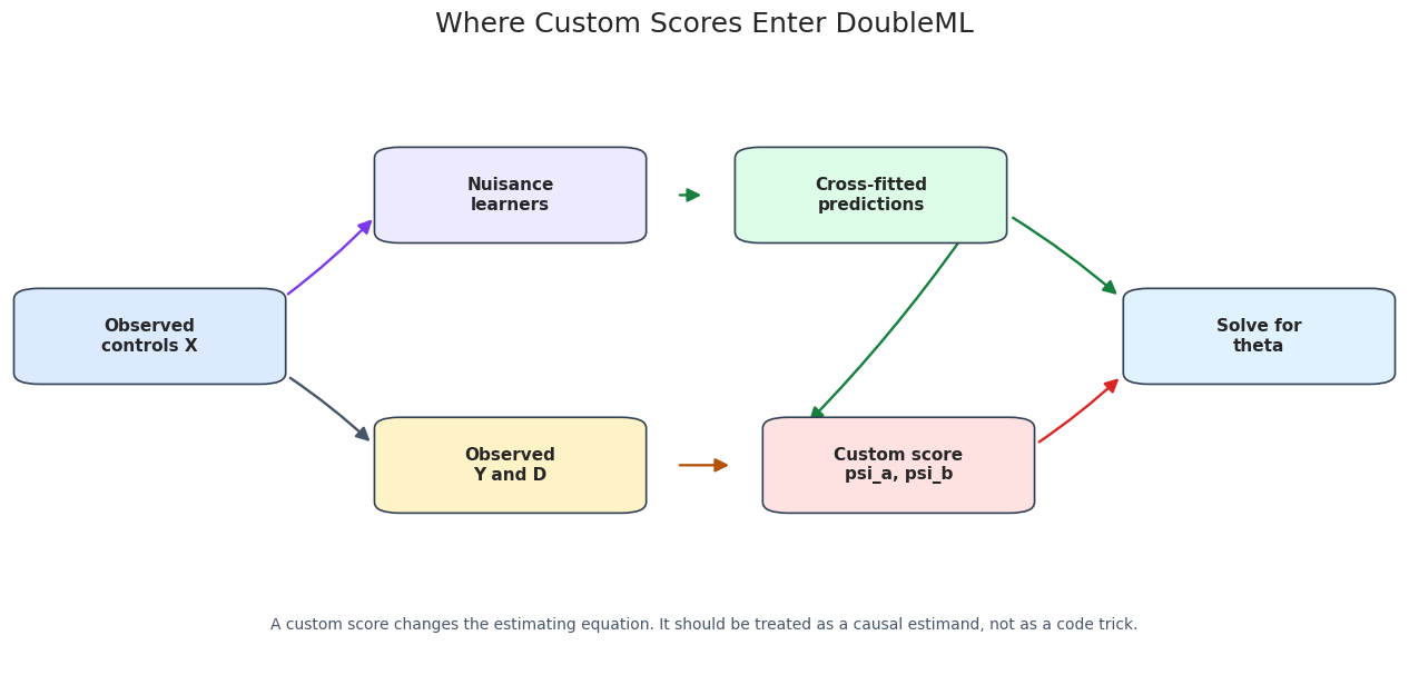
Score Design Diagram

The diagram below shows where a custom score enters DoubleML. Nuisance learners produce cross-fitted predictions. The score function turns observed data and nuisance predictions into psi_a and psi_b. DoubleML then solves the empirical score equation.

fig, ax = plt.subplots(figsize=(13, 6.5))
ax.set_axis_off()

nodes = {
    "X": {"xy": (0.10, 0.55), "label": "Observed\ncontrols X", "color": "#dbeafe"},
    "N": {"xy": (0.36, 0.78), "label": "Nuisance\nlearners", "color": "#ede9fe"},
    "P": {"xy": (0.62, 0.78), "label": "Cross-fitted\npredictions", "color": "#dcfce7"},
    "W": {"xy": (0.36, 0.34), "label": "Observed\nY and D", "color": "#fef3c7"},
    "S": {"xy": (0.64, 0.34), "label": "Custom score\npsi_a, psi_b", "color": "#fee2e2"},
    "T": {"xy": (0.90, 0.55), "label": "Solve for\ntheta", "color": "#e0f2fe"},
}

box_w, box_h = 0.16, 0.12


def anchor(node, side):
    x, y = nodes[node]["xy"]
    offsets = {
        "left": (-box_w / 2, 0),
        "right": (box_w / 2, 0),
        "top": (0, box_h / 2),
        "bottom": (0, -box_h / 2),
        "upper_right": (box_w / 2, box_h * 0.25),
        "lower_right": (box_w / 2, -box_h * 0.25),
        "upper_left": (-box_w / 2, box_h * 0.25),
        "lower_left": (-box_w / 2, -box_h * 0.25),
    }
    dx, dy = offsets[side]
    return np.array([x + dx, y + dy], dtype=float)


def shorten(start, end, gap=0.040):
    start = np.asarray(start, dtype=float)
    end = np.asarray(end, dtype=float)
    delta = end - start
    length = np.hypot(delta[0], delta[1])
    if length == 0:
        return tuple(start), tuple(end)
    unit = delta / length
    return tuple(start + gap * unit), tuple(end - gap * unit)


def draw_arrow(start, end, color="#334155", style="solid", rad=0.0, linewidth=1.7):
    start, end = shorten(start, end)
    arrow = FancyArrowPatch(
        start,
        end,
        arrowstyle="-|>",
        mutation_scale=18,
        linewidth=linewidth,
        color=color,
        linestyle=style,
        connectionstyle=f"arc3,rad={rad}",
        zorder=2,
        clip_on=False,
    )
    ax.add_patch(arrow)

draw_arrow(anchor("X", "upper_right"), anchor("N", "left"), color="#7c3aed", rad=0.04)
draw_arrow(anchor("N", "right"), anchor("P", "left"), color="#15803d")
draw_arrow(anchor("X", "lower_right"), anchor("W", "left"), color="#475569", rad=-0.04)
draw_arrow(anchor("P", "lower_right"), anchor("S", "upper_left"), color="#15803d", rad=-0.04)
draw_arrow(anchor("W", "right"), anchor("S", "left"), color="#b45309")
draw_arrow(anchor("S", "right"), anchor("T", "lower_left"), color="#dc2626", rad=0.04)
draw_arrow(anchor("P", "right"), anchor("T", "upper_left"), color="#15803d", rad=-0.04)

for spec in nodes.values():
    x, y = spec["xy"]
    rect = FancyBboxPatch(
        (x - box_w / 2, y - box_h / 2),
        box_w,
        box_h,
        boxstyle="round,pad=0.018",
        facecolor=spec["color"],
        edgecolor="#334155",
        linewidth=1.2,
        zorder=3,
    )
    ax.add_patch(rect)
    ax.text(x, y, spec["label"], ha="center", va="center", fontsize=11, fontweight="bold", zorder=4)

ax.text(
    0.50,
    0.08,
    "A custom score changes the estimating equation. It should be treated as a causal estimand, not as a code trick.",
    ha="center",
    va="center",
    fontsize=10,
    color="#475569",
)
ax.set_title("Where Custom Scores Enter DoubleML", pad=18)
plt.tight_layout()
fig.savefig(FIGURE_DIR / f"{NOTEBOOK_PREFIX}_custom_score_design.png", dpi=160, bbox_inches="tight")
plt.show()

The score function is downstream of nuisance prediction but upstream of the final coefficient. This is why custom-score work needs both statistical theory and software testing.

External Sample Splits

For a fair comparison between built-in and custom scores, we fix the sample split. This makes the nuisance predictions comparable across model variants.

sample_splits = list(KFold(n_splits=5, shuffle=True, random_state=RANDOM_SEED + 2).split(plr_df))
fold_id = np.full(len(plr_df), -1)
for fold_number, (_, test_index) in enumerate(sample_splits):
    fold_id[test_index] = fold_number

split_summary = pd.DataFrame(
    {
        "fold": np.arange(len(sample_splits)),
        "test_rows": [len(test_index) for _, test_index in sample_splits],
        "train_rows": [len(train_index) for train_index, _ in sample_splits],
    }
)

save_table(split_summary, f"{NOTEBOOK_PREFIX}_sample_split_summary.csv")
display(split_summary)

	fold	test_rows	train_rows
0	0	180	720
1	1	180	720
2	2	180	720
3	3	180	720
4	4	180	720

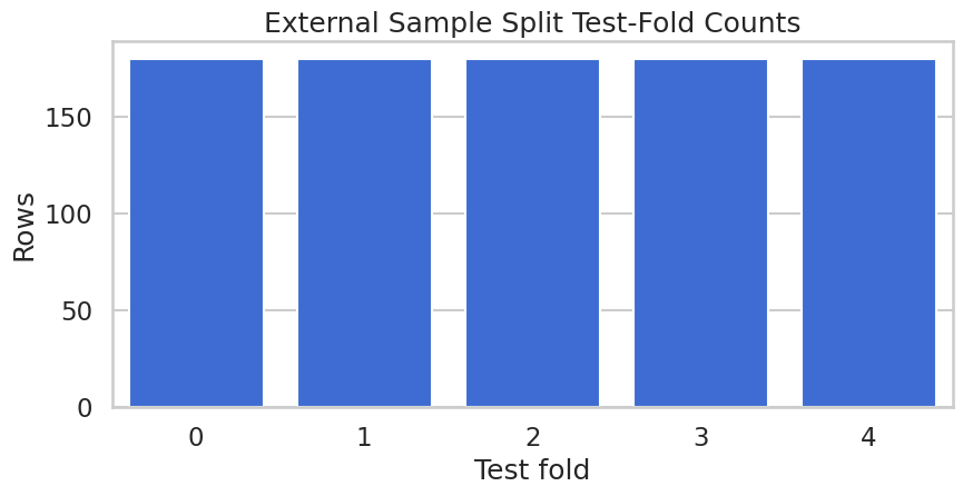
Every row appears in exactly one test fold. This is the cross-fitting structure that lets each score contribution use nuisance predictions from a model that did not train on that row.

Plot Fold Assignments

The plot below is a simple audit of the external fold assignment. It is not mathematically necessary, but it makes the custom split visible.

fig, ax = plt.subplots(figsize=(9, 4.8))
sns.countplot(x=fold_id, color="#2563eb", ax=ax)
ax.set_title("External Sample Split Test-Fold Counts")
ax.set_xlabel("Test fold")
ax.set_ylabel("Rows")
plt.tight_layout()
fig.savefig(FIGURE_DIR / f"{NOTEBOOK_PREFIX}_external_sample_split_counts.png", dpi=160, bbox_inches="tight")
plt.show()

The fold sizes are balanced. If the split were grouped or temporal, this same table and plot would be useful for checking whether the split design matches the causal setting.

Fit The Built-In PLR Score

We first fit the standard partialling out PLR score. This is the reference model for the custom score examples.

base_learner = RandomForestRegressor(
    n_estimators=80,
    max_depth=6,
    min_samples_leaf=10,
    random_state=RANDOM_SEED + 1,
    n_jobs=-1,
)

builtin_plr = fit_plr(
    plr_df,
    x_cols,
    learner_l=base_learner,
    learner_m=base_learner,
    score="partialling out",
    sample_splits=sample_splits,
    store_models=True,
)

builtin_result = pd.DataFrame([extract_plr_row("Built-in partialling out", builtin_plr)])
save_table(builtin_result, f"{NOTEBOOK_PREFIX}_builtin_plr_result.csv")
display(builtin_result)

	model	estimate	std_error	ci_95_lower	ci_95_upper	true_theta	absolute_error
0	Built-in partialling out	1.2852	0.0359	1.2148	1.3556	1.2500	0.0352

The built-in model estimates the true constant treatment effect closely. This gives us a reliable baseline for testing custom score behavior.

Reconstruct The Estimate From Score Elements

DoubleML stores psi_a and psi_b. For a linear score, the fitted coefficient is the value that makes the average final score approximately zero:

\[ \frac{1}{n}\sum_{i=1}^{n} \left(\psi_{a,i}\hat{\theta} + \psi_{b,i}\right) \approx 0. \]

Solving that equation gives:

\[ \hat{\theta} = -\frac{\bar{\psi}_b}{\bar{\psi}_a}, \qquad \bar{\psi}_a = \frac{1}{n}\sum_{i=1}^{n}\psi_{a,i}, \qquad \bar{\psi}_b = \frac{1}{n}\sum_{i=1}^{n}\psi_{b,i}. \]

This cell reconstructs the coefficient directly from the stored score elements. It is a useful sanity check before writing a custom score because it confirms that the notebook is reading DoubleML’s internal score representation correctly.

builtin_psi_a = builtin_plr.psi_elements["psi_a"].reshape(-1)
builtin_psi_b = builtin_plr.psi_elements["psi_b"].reshape(-1)
reconstructed_theta = solve_linear_score(builtin_psi_a, builtin_psi_b)

score_reconstruction = pd.DataFrame(
    [
        {"calculation": "DoubleML coefficient", "value": float(builtin_plr.coef[0])},
        {"calculation": "-mean(psi_b) / mean(psi_a)", "value": reconstructed_theta},
        {"calculation": "True theta", "value": TRUE_THETA},
        {"calculation": "mean(psi_a)", "value": float(np.mean(builtin_psi_a))},
        {"calculation": "mean(psi_b)", "value": float(np.mean(builtin_psi_b))},
    ]
)

save_table(score_reconstruction, f"{NOTEBOOK_PREFIX}_score_reconstruction.csv")
display(score_reconstruction)

	calculation	value
0	DoubleML coefficient	1.2852
1	-mean(psi_b) / mean(psi_a)	1.2852
2	True theta	1.2500
3	mean(psi_a)	-1.1032
4	mean(psi_b)	1.4178

The first two rows match because the linear score equation is exactly how the coefficient is obtained. This is the mental model needed before writing a custom score.

Nuisance-Model Diagnostics

Before changing the score, we check the nuisance learners. Bad nuisance predictions can make even a valid score unstable in finite samples.

learner_rmse = builtin_plr.evaluate_learners(metric=lambda y_true, y_pred: np.sqrt(mean_squared_error(y_true, y_pred)))
learner_mae = builtin_plr.evaluate_learners(metric=mean_absolute_error)

nuisance_diagnostics = pd.DataFrame(
    [
        {"learner": "ml_l", "metric": "RMSE", "value": float(learner_rmse["ml_l"][0, 0])},
        {"learner": "ml_m", "metric": "RMSE", "value": float(learner_rmse["ml_m"][0, 0])},
        {"learner": "ml_l", "metric": "MAE", "value": float(learner_mae["ml_l"][0, 0])},
        {"learner": "ml_m", "metric": "MAE", "value": float(learner_mae["ml_m"][0, 0])},
    ]
)

save_table(nuisance_diagnostics, f"{NOTEBOOK_PREFIX}_nuisance_diagnostics.csv")
display(nuisance_diagnostics)

	learner	metric	value
0	ml_l	RMSE	1.7981
1	ml_m	RMSE	1.0503
2	ml_l	MAE	1.4433
3	ml_m	MAE	0.8334

The nuisance metrics are not causal proof, but they tell us whether the first-stage models are at least numerically plausible before score-level work begins.

Callable Score Equivalent To Built-In Partialling Out

Now we write the PLR partialling-out score by hand. The callable signature for DoubleMLPLR is still a Python API contract:

score(y, d, l_hat, m_hat, g_hat, smpls) -> psi_a, psi_b

For the partialling-out score, the residualized treatment and residualized outcome are:

\[ \hat{v}_i = d_i - \hat{m}(x_i), \qquad \hat{u}_i = y_i - \hat{\ell}(x_i). \]

The linear score pieces are:

\[ \psi_{a,i} = -\hat{v}_i^2, \qquad \psi_{b,i} = \hat{v}_i\hat{u}_i. \]

So the final observation-level score is:

\[ \psi_i(\theta) = -\hat{v}_i^2\theta + \hat{v}_i\hat{u}_i. \]

If the callable is correct and we use the same folds and learners, it should match the built-in score.

def partialling_out_callable(y, d, l_hat, m_hat, g_hat, smpls):
    v_hat = d - m_hat
    u_hat = y - l_hat
    psi_a = -v_hat * v_hat
    psi_b = v_hat * u_hat
    return psi_a, psi_b

callable_plr = fit_plr(
    plr_df,
    x_cols,
    learner_l=base_learner,
    learner_m=base_learner,
    score=partialling_out_callable,
    sample_splits=sample_splits,
)

callable_result = pd.DataFrame([extract_plr_row("Callable partialling out", callable_plr)])
save_table(callable_result, f"{NOTEBOOK_PREFIX}_callable_plr_result.csv")
display(callable_result)

	model	estimate	std_error	ci_95_lower	ci_95_upper	true_theta	absolute_error
0	Callable partialling out	1.2852	0.0359	1.2148	1.3556	1.2500	0.0352

The callable score reproduces the built-in estimate. This is the safest first custom-score test: before extending a score, verify that you can recreate a known one.

Priority-Weighted Callable Score

This example multiplies the score contributions by a pre-treatment priority weight. The weighted score is:

\[ \psi_i^{(w)}(\theta) = w_i\left(-\hat{v}_i^2\theta + \hat{v}_i\hat{u}_i\right), \]

which is equivalent to returning:

\[ \psi_{a,i}^{(w)} = -w_i\hat{v}_i^2, \qquad \psi_{b,i}^{(w)} = w_i\hat{v}_i\hat{u}_i. \]

Because the true effect is constant in this simulator, the causal parameter remains TRUE_THETA; the weighting changes finite-sample influence rather than creating a different heterogeneous estimand. In a real analysis, the weight definition should be pre-specified and justified. Weighting is not a free way to find a more convenient answer.

priority_weights = normalize_weights(1.0 + 1.50 * plr_df["priority_segment"].eq("high_priority").astype(float))


def make_priority_weighted_score(weights):
    weights = np.asarray(weights, dtype=float)

    def priority_weighted_score(y, d, l_hat, m_hat, g_hat, smpls):
        v_hat = d - m_hat
        u_hat = y - l_hat
        psi_a = -weights * v_hat * v_hat
        psi_b = weights * v_hat * u_hat
        return psi_a, psi_b

    return priority_weighted_score

weighted_plr = fit_plr(
    plr_df,
    x_cols,
    learner_l=base_learner,
    learner_m=base_learner,
    score=make_priority_weighted_score(priority_weights),
    sample_splits=sample_splits,
)

weighted_result = pd.DataFrame([extract_plr_row("Priority-weighted callable score", weighted_plr)])
save_table(weighted_result, f"{NOTEBOOK_PREFIX}_weighted_callable_result.csv")
display(weighted_result)

	model	estimate	std_error	ci_95_lower	ci_95_upper	true_theta	absolute_error
0	Priority-weighted callable score	1.2890	0.0381	1.2144	1.3636	1.2500	0.0390

The weighted estimate stays close to the true constant effect. A large shift would not automatically be wrong, but it would require a clear explanation of what target changed and why.

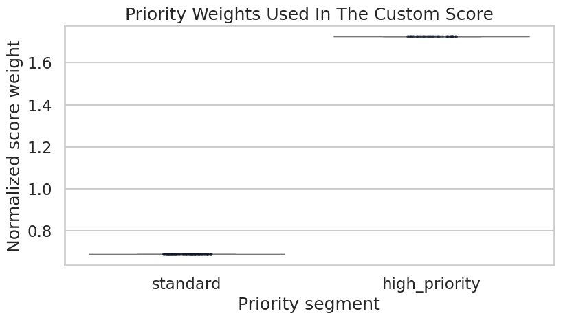
Plot Priority Weights

The plot below documents the weighting rule. Showing the weight distribution is a simple way to make custom scores less mysterious.

weight_plot_df = plr_df[["priority_segment"]].assign(priority_weight=priority_weights)

fig, ax = plt.subplots(figsize=(8.5, 5))
sns.boxplot(data=weight_plot_df, x="priority_segment", y="priority_weight", color="#93c5fd", ax=ax)
sns.stripplot(data=weight_plot_df.sample(250, random_state=RANDOM_SEED), x="priority_segment", y="priority_weight", color="#111827", alpha=0.35, size=3, ax=ax)
ax.set_title("Priority Weights Used In The Custom Score")
ax.set_xlabel("Priority segment")
ax.set_ylabel("Normalized score weight")
plt.tight_layout()
fig.savefig(FIGURE_DIR / f"{NOTEBOOK_PREFIX}_priority_weights.png", dpi=160, bbox_inches="tight")
plt.show()

The high-priority group receives larger score weight by design. Since the weights are normalized, the average weight is one.

A Deliberately Bad Score As A Caution

This cell fits a non-orthogonal raw score that ignores the treatment nuisance model and does not residualize the treatment. The goal is not to recommend this score. The goal is to show that DoubleML will execute a callable score if it has the right shape, but it cannot prove that the score is a valid causal moment.

def nonorthogonal_raw_score(y, d, l_hat, m_hat, g_hat, smpls):
    psi_a = -d * d
    psi_b = d * y
    return psi_a, psi_b

bad_score_plr = fit_plr(
    plr_df,
    x_cols,
    learner_l=base_learner,
    learner_m=base_learner,
    score=nonorthogonal_raw_score,
    sample_splits=sample_splits,
)

bad_score_result = pd.DataFrame([extract_plr_row("Non-orthogonal raw score caution", bad_score_plr)])
save_table(bad_score_result, f"{NOTEBOOK_PREFIX}_bad_score_caution.csv")
display(bad_score_result)

	model	estimate	std_error	ci_95_lower	ci_95_upper	true_theta	absolute_error
0	Non-orthogonal raw score caution	1.3535	0.0316	1.2917	1.4154	1.2500	0.1035

The cautionary score is farther from the known truth. The lesson is sharp: a callable score is an API hook, not a validity certificate.

Compare Score Variants

This table combines the built-in score, equivalent callable score, priority-weighted score, and cautionary raw score.

score_comparison = pd.concat(
    [builtin_result, callable_result, weighted_result, bad_score_result],
    ignore_index=True,
)
score_comparison = score_comparison.sort_values("absolute_error")

save_table(score_comparison, f"{NOTEBOOK_PREFIX}_score_variant_comparison.csv")
display(score_comparison)

	model	estimate	std_error	ci_95_lower	ci_95_upper	true_theta	absolute_error
0	Built-in partialling out	1.2852	0.0359	1.2148	1.3556	1.2500	0.0352
1	Callable partialling out	1.2852	0.0359	1.2148	1.3556	1.2500	0.0352
2	Priority-weighted callable score	1.2890	0.0381	1.2144	1.3636	1.2500	0.0390
3	Non-orthogonal raw score caution	1.3535	0.0316	1.2917	1.4154	1.2500	0.1035

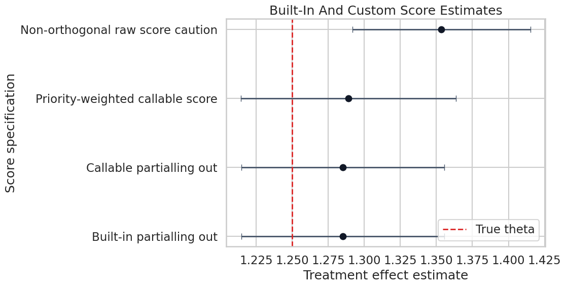
The built-in and equivalent callable scores match. The priority-weighted score remains close. The raw non-orthogonal score is a useful warning about custom-score responsibility.

Plot Score Variant Estimates

The estimate plot makes the custom-score comparison easier to scan. The vertical line marks the true effect in the simulation.

plot_scores = score_comparison.sort_values("estimate")
y_positions = np.arange(len(plot_scores))

fig, ax = plt.subplots(figsize=(11.5, 6))
ax.errorbar(
    x=plot_scores["estimate"],
    y=y_positions,
    xerr=np.vstack([
        plot_scores["estimate"] - plot_scores["ci_95_lower"],
        plot_scores["ci_95_upper"] - plot_scores["estimate"],
    ]),
    fmt="o",
    color="#111827",
    ecolor="#475569",
    elinewidth=2,
    capsize=4,
)
ax.axvline(TRUE_THETA, color="#dc2626", linestyle="--", linewidth=2, label="True theta")
ax.set_yticks(y_positions)
ax.set_yticklabels(plot_scores["model"])
ax.set_title("Built-In And Custom Score Estimates")
ax.set_xlabel("Treatment effect estimate")
ax.set_ylabel("Score specification")
ax.legend(loc="lower right")
plt.tight_layout()
fig.savefig(FIGURE_DIR / f"{NOTEBOOK_PREFIX}_score_variant_estimates.png", dpi=160, bbox_inches="tight")
plt.show()

The plot helps separate extension from experimentation. A custom score should be expected to behave in a known way; surprising movement is a reason to inspect the score, not a reason to celebrate.

Score Contribution Diagnostics

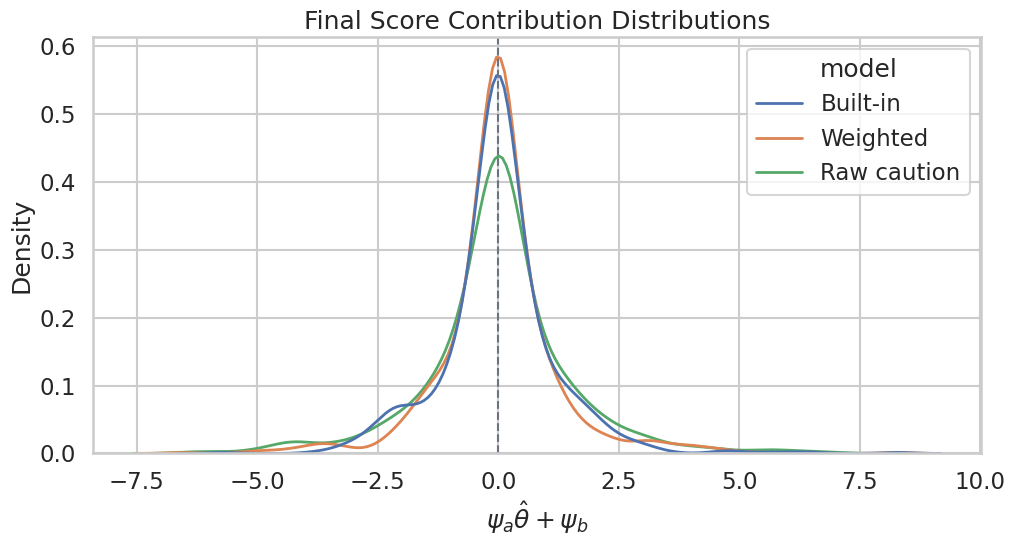
The next cell extracts score contributions from the built-in and custom models. After plugging in the fitted coefficient, the final score contribution is:

\[ \hat{\psi}_i = \psi_{a,i}\hat{\theta} + \psi_{b,i}. \]

For a successfully solved linear score, the empirical mean should be near zero:

\[ \frac{1}{n}\sum_{i=1}^{n}\hat{\psi}_i \approx 0. \]

We compare the score-implied coefficient and the spread of \(\hat{\psi}_i\). The mean checks whether the moment equation was solved; the spread and tails help identify unstable score behavior.

def score_diagnostic_row(label, model):
    psi_a = model.psi_elements["psi_a"].reshape(-1)
    psi_b = model.psi_elements["psi_b"].reshape(-1)
    theta = float(model.coef[0])
    final_score = psi_a * theta + psi_b
    return {
        "model": label,
        "theta_from_score_elements": solve_linear_score(psi_a, psi_b),
        "mean_final_score": float(np.mean(final_score)),
        "std_final_score": float(np.std(final_score)),
        "score_p01": float(np.quantile(final_score, 0.01)),
        "score_p99": float(np.quantile(final_score, 0.99)),
    }

score_diagnostics = pd.DataFrame(
    [
        score_diagnostic_row("Built-in partialling out", builtin_plr),
        score_diagnostic_row("Callable partialling out", callable_plr),
        score_diagnostic_row("Priority-weighted callable score", weighted_plr),
        score_diagnostic_row("Non-orthogonal raw score caution", bad_score_plr),
    ]
)

save_table(score_diagnostics, f"{NOTEBOOK_PREFIX}_score_diagnostics.csv")
display(score_diagnostics)

	model	theta_from_score_elements	mean_final_score	std_final_score	score_p01	score_p99
0	Built-in partialling out	1.2852	0.0000	1.1885	-2.9024	3.0922
1	Callable partialling out	1.2852	0.0000	1.1885	-2.9024	3.0922
2	Priority-weighted callable score	1.2890	-0.0000	1.2416	-3.8380	3.9954
3	Non-orthogonal raw score caution	1.3535	0.0000	1.5268	-4.4432	4.6343

The mean final score is near zero because the estimate solves the empirical moment equation. The spread and tails help identify unstable score behavior.

Plot Score Contributions

The histogram below compares final score contributions after plugging in each model’s estimated coefficient.

score_distribution_df = pd.concat(
    [
        pd.DataFrame({"model": "Built-in", "final_score": builtin_plr.psi_elements["psi_a"].reshape(-1) * builtin_plr.coef[0] + builtin_plr.psi_elements["psi_b"].reshape(-1)}),
        pd.DataFrame({"model": "Weighted", "final_score": weighted_plr.psi_elements["psi_a"].reshape(-1) * weighted_plr.coef[0] + weighted_plr.psi_elements["psi_b"].reshape(-1)}),
        pd.DataFrame({"model": "Raw caution", "final_score": bad_score_plr.psi_elements["psi_a"].reshape(-1) * bad_score_plr.coef[0] + bad_score_plr.psi_elements["psi_b"].reshape(-1)}),
    ],
    ignore_index=True,
)

fig, ax = plt.subplots(figsize=(10.5, 5.8))
sns.kdeplot(
    data=score_distribution_df,
    x="final_score",
    hue="model",
    common_norm=False,
    linewidth=2,
    ax=ax,
)
ax.axvline(0, color="#6b7280", linestyle="--", linewidth=1.5)
ax.set_title("Final Score Contribution Distributions")
ax.set_xlabel(r"$\psi_a \hat{\theta} + \psi_b$")
ax.set_ylabel("Density")
plt.tight_layout()
fig.savefig(FIGURE_DIR / f"{NOTEBOOK_PREFIX}_score_contribution_distributions.png", dpi=160, bbox_inches="tight")
plt.show()

Score distributions with extreme tails deserve attention. In applied work, this can point to overlap problems, unstable residualized treatment, or a score that is not well matched to the design.

External Nuisance Predictions

DoubleML can accept nuisance predictions from an external ML pipeline. For PLR, the nested dictionary shape is:

{
    "treatment": {
        "ml_l": array_of_l_hat_with_shape_(n_obs, n_rep),
        "ml_m": array_of_m_hat_with_shape_(n_obs, n_rep),
    }
}

Here we create the external predictions manually using the same folds. This mirrors how a production ML team might supply predictions while the causal analysis team uses DoubleML for score estimation and inference.

external_l_hat, external_m_hat = manual_cross_fit_predictions(
    plr_df,
    x_cols,
    sample_splits,
    learner_l=base_learner,
    learner_m=base_learner,
)

external_predictions = {
    "treatment": {
        "ml_l": external_l_hat.reshape(-1, 1),
        "ml_m": external_m_hat.reshape(-1, 1),
    }
}

external_prediction_model = fit_plr(
    plr_df,
    x_cols,
    learner_l=base_learner,
    learner_m=base_learner,
    score="partialling out",
    sample_splits=sample_splits,
    external_predictions=external_predictions,
)

external_prediction_result = pd.DataFrame([extract_plr_row("External nuisance predictions", external_prediction_model)])
save_table(external_prediction_result, f"{NOTEBOOK_PREFIX}_external_prediction_result.csv")
display(external_prediction_result)

	model	estimate	std_error	ci_95_lower	ci_95_upper	true_theta	absolute_error
0	External nuisance predictions	1.2852	0.0359	1.2148	1.3556	1.2500	0.0352

The external-prediction estimate matches the built-in pipeline because the same folds and same learners generated the predictions. This is the desired smoke test before connecting a more complex external pipeline.

Compare Internal And External Predictions

This cell checks that the manually supplied external predictions match the predictions stored by the built-in DoubleML fit.

internal_l_hat = builtin_plr.predictions["ml_l"][:, 0, 0]
internal_m_hat = builtin_plr.predictions["ml_m"][:, 0, 0]

external_prediction_audit = pd.DataFrame(
    [
        {"prediction": "ml_l", "max_abs_difference": float(np.max(np.abs(internal_l_hat - external_l_hat))), "rmse_difference": rmse(internal_l_hat, external_l_hat)},
        {"prediction": "ml_m", "max_abs_difference": float(np.max(np.abs(internal_m_hat - external_m_hat))), "rmse_difference": rmse(internal_m_hat, external_m_hat)},
        {"prediction": "theta", "max_abs_difference": abs(float(builtin_plr.coef[0]) - float(external_prediction_model.coef[0])), "rmse_difference": np.nan},
    ]
)

save_table(external_prediction_audit, f"{NOTEBOOK_PREFIX}_external_prediction_audit.csv")
display(external_prediction_audit)

	prediction	max_abs_difference	rmse_difference
0	ml_l	0.0000	0.0000
1	ml_m	0.0000	0.0000
2	theta	0.0000	NaN

The differences are zero or numerically tiny. This confirms the dictionary shape and row order are correct.

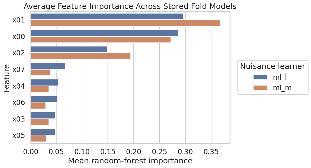
Stored Fold Models And Feature Importance

With store_models=True, DoubleML keeps the fold-level nuisance models. This cell extracts average random-forest feature importance across the stored ml_l and ml_m models.

importance_rows = []
for learner_name in ["ml_l", "ml_m"]:
    fold_models = builtin_plr.models[learner_name]["treatment"][0]
    for fold_number, model in enumerate(fold_models):
        for feature, importance in zip(x_cols, model.feature_importances_):
            importance_rows.append(
                {
                    "learner": learner_name,
                    "fold": fold_number,
                    "feature": feature,
                    "importance": float(importance),
                }
            )

feature_importance = pd.DataFrame(importance_rows)
feature_importance_summary = (
    feature_importance.groupby(["learner", "feature"])
    .agg(mean_importance=("importance", "mean"), std_importance=("importance", "std"))
    .reset_index()
    .sort_values(["learner", "mean_importance"], ascending=[True, False])
)

save_table(feature_importance_summary, f"{NOTEBOOK_PREFIX}_stored_model_feature_importance.csv")
display(feature_importance_summary.head(12))

	learner	feature	mean_importance	std_importance
1	ml_l	x01	0.2959	0.0219
0	ml_l	x00	0.2863	0.0148
2	ml_l	x02	0.1494	0.0221
7	ml_l	x07	0.0674	0.0125
4	ml_l	x04	0.0538	0.0068
6	ml_l	x06	0.0515	0.0073
3	ml_l	x03	0.0485	0.0117
5	ml_l	x05	0.0472	0.0124
9	ml_m	x01	0.3679	0.0235
8	ml_m	x00	0.2717	0.0070
10	ml_m	x02	0.1926	0.0294
15	ml_m	x07	0.0376	0.0047

Stored fold models are useful for auditing, but feature importance is still an ML diagnostic. It does not prove causal importance of a covariate.

Plot Stored-Model Feature Importance

The plot below compares the nuisance models for outcome and treatment. Different important features are expected because ml_l predicts Y and ml_m predicts D.

fig, ax = plt.subplots(figsize=(10.5, 5.8))
sns.barplot(
    data=feature_importance_summary,
    x="mean_importance",
    y="feature",
    hue="learner",
    ax=ax,
)
ax.set_title("Average Feature Importance Across Stored Fold Models")
ax.set_xlabel("Mean random-forest importance")
ax.set_ylabel("Feature")
ax.legend(title="Nuisance learner", loc="center left", bbox_to_anchor=(1.02, 0.5))
plt.tight_layout()
fig.savefig(FIGURE_DIR / f"{NOTEBOOK_PREFIX}_stored_model_feature_importance.png", dpi=160, bbox_inches="tight")
plt.show()

The treatment model emphasizes features involved in true_m, while the outcome model emphasizes features involved in both outcome prediction and treatment-related variation. This is a useful sanity check against the simulator.

Custom Score Validation Checklist

The table below converts the notebook into a checklist. A custom score should not be merged into a serious analysis until it passes checks like these.

custom_score_checklist = pd.DataFrame(
    [
        {"check": "Known-score recreation", "guidance": "First recreate a built-in score exactly using the callable interface."},
        {"check": "Shape check", "guidance": "Confirm psi_a and psi_b are finite arrays aligned with the original row order."},
        {"check": "Moment check", "guidance": "Verify that mean(psi_a * theta_hat + psi_b) is approximately zero."},
        {"check": "Orthogonality argument", "guidance": "Write the mathematical reason why nuisance errors have only second-order impact."},
        {"check": "Split reproducibility", "guidance": "Use fixed sample splits when comparing scores or external predictions."},
        {"check": "External prediction audit", "guidance": "Check row order, shape, and fold origin of external nuisance predictions."},
        {"check": "Unsupported features", "guidance": "Document DoubleML features unavailable for callable scores, such as sensitivity analysis in this version."},
        {"check": "Simulation test", "guidance": "Test the score on data where the truth is known before using it on real data."},
    ]
)

save_table(custom_score_checklist, f"{NOTEBOOK_PREFIX}_custom_score_validation_checklist.csv")
display(custom_score_checklist)

	check	guidance
0	Known-score recreation	First recreate a built-in score exactly using ...
1	Shape check	Confirm psi_a and psi_b are finite arrays alig...
2	Moment check	Verify that mean(psi_a * theta_hat + psi_b) is...
3	Orthogonality argument	Write the mathematical reason why nuisance err...
4	Split reproducibility	Use fixed sample splits when comparing scores ...
5	External prediction audit	Check row order, shape, and fold origin of ext...
6	Unsupported features	Document DoubleML features unavailable for cal...
7	Simulation test	Test the score on data where the truth is know...

The checklist is deliberately stricter than merely running without errors. Custom scores are extension points, so the burden of proof moves to the analyst.

Advanced API Summary

This table summarizes the advanced APIs used in the notebook and the caution attached to each.

advanced_api_summary = pd.DataFrame(
    [
        {"api": "score=callable", "used_for": "Custom score elements", "main_caution": "DoubleML checks shape and execution, not causal validity."},
        {"api": "set_sample_splitting()", "used_for": "Reproducible fold assignment", "main_caution": "The split must match the data design; random folds are not always appropriate."},
        {"api": "external_predictions", "used_for": "Supplying nuisance predictions", "main_caution": "Predictions must be cross-fitted, row-aligned, and shaped as (n_obs, n_rep)."},
        {"api": "store_models=True", "used_for": "Auditing fitted nuisance models", "main_caution": "Model diagnostics are not causal evidence."},
        {"api": "psi_elements", "used_for": "Score reconstruction and diagnostics", "main_caution": "Score diagnostics can reveal instability but do not replace identification assumptions."},
        {"api": "evaluate_learners()", "used_for": "Out-of-fold nuisance loss", "main_caution": "Low predictive loss is helpful but not sufficient for causal credibility."},
    ]
)

save_table(advanced_api_summary, f"{NOTEBOOK_PREFIX}_advanced_api_summary.csv")
display(advanced_api_summary)

	api	used_for	main_caution
0	score=callable	Custom score elements	DoubleML checks shape and execution, not causa...
1	set_sample_splitting()	Reproducible fold assignment	The split must match the data design; random f...
2	external_predictions	Supplying nuisance predictions	Predictions must be cross-fitted, row-aligned,...
3	store_models=True	Auditing fitted nuisance models	Model diagnostics are not causal evidence.
4	psi_elements	Score reconstruction and diagnostics	Score diagnostics can reveal instability but d...
5	evaluate_learners()	Out-of-fold nuisance loss	Low predictive loss is helpful but not suffici...

The advanced API is powerful because it lets DoubleML interoperate with custom ML and custom moments. That same flexibility is why documentation and testing are part of the analysis, not an afterthought.

Write A Reusable Report Template

This report template captures how a custom-score analysis should be documented.

report_template = rf"""# Custom Score And Advanced DoubleML API Report Template

## Causal Estimand
State the target parameter and the model assumptions. Explain why a built-in DoubleML score is or is not sufficient.

## Score Definition
Write the score as $\psi(W; \theta, \eta) = \psi_a(W; \eta)\theta + \psi_b(W; \eta)$. Include the callable function signature and all nuisance inputs.

## Orthogonality Argument
Explain why the score is Neyman-orthogonal. If the score is not orthogonal, do not present it as a DoubleML-style robust estimator.

## Reproducibility Checks
Document sample splitting, random seeds, learner settings, and whether external nuisance predictions were supplied.

## Validation Results
Report known-score recreation, score reconstruction, final score mean, nuisance diagnostics, and any simulation checks with known truth.

## Unsupported Or Limited Features
Document any DoubleML features that are unavailable for callable scores in the installed version.

## Decision Boundary
State what the custom score supports and what still needs theory, robustness checks, or experimental validation.

Key estimate from this notebook:
- Built-in PLR estimate: {float(builtin_plr.coef[0]):.4f}
- Callable equivalent estimate: {float(callable_plr.coef[0]):.4f}
- Priority-weighted callable estimate: {float(weighted_plr.coef[0]):.4f}
- True $\theta_0$ in simulation: {TRUE_THETA:.4f}
"""

report_path = REPORT_DIR / f"{NOTEBOOK_PREFIX}_custom_score_report_template.md"
report_path.write_text(report_template)

print(f"Wrote report template to: {report_path}")

Wrote report template to: /home/apex/Documents/ranking_sys/notebooks/tutorials/doubleml/outputs/reports/16_custom_score_report_template.md

The template forces the custom score to be documented mathematically and operationally. That is exactly the habit this notebook is trying to build.

Artifact Manifest

The manifest below lists the main artifacts written by this notebook.

artifact_manifest = pd.DataFrame(
    [
        {"artifact": "Synthetic PLR dataset", "path": str(DATASET_DIR / f"{NOTEBOOK_PREFIX}_synthetic_custom_score_plr_data.csv")},
        {"artifact": "Score variant comparison", "path": str(TABLE_DIR / f"{NOTEBOOK_PREFIX}_score_variant_comparison.csv")},
        {"artifact": "Score diagnostics", "path": str(TABLE_DIR / f"{NOTEBOOK_PREFIX}_score_diagnostics.csv")},
        {"artifact": "External prediction audit", "path": str(TABLE_DIR / f"{NOTEBOOK_PREFIX}_external_prediction_audit.csv")},
        {"artifact": "Stored-model feature importance", "path": str(TABLE_DIR / f"{NOTEBOOK_PREFIX}_stored_model_feature_importance.csv")},
        {"artifact": "Custom score checklist", "path": str(TABLE_DIR / f"{NOTEBOOK_PREFIX}_custom_score_validation_checklist.csv")},
        {"artifact": "Report template", "path": str(REPORT_DIR / f"{NOTEBOOK_PREFIX}_custom_score_report_template.md")},
        {"artifact": "Custom score design figure", "path": str(FIGURE_DIR / f"{NOTEBOOK_PREFIX}_custom_score_design.png")},
        {"artifact": "Score estimate figure", "path": str(FIGURE_DIR / f"{NOTEBOOK_PREFIX}_score_variant_estimates.png")},
        {"artifact": "Score contribution figure", "path": str(FIGURE_DIR / f"{NOTEBOOK_PREFIX}_score_contribution_distributions.png")},
    ]
)

save_table(artifact_manifest, f"{NOTEBOOK_PREFIX}_artifact_manifest.csv")
display(artifact_manifest)

	artifact	path
0	Synthetic PLR dataset	/home/apex/Documents/ranking_sys/notebooks/tut...
1	Score variant comparison	/home/apex/Documents/ranking_sys/notebooks/tut...
2	Score diagnostics	/home/apex/Documents/ranking_sys/notebooks/tut...
3	External prediction audit	/home/apex/Documents/ranking_sys/notebooks/tut...
4	Stored-model feature importance	/home/apex/Documents/ranking_sys/notebooks/tut...
5	Custom score checklist	/home/apex/Documents/ranking_sys/notebooks/tut...
6	Report template	/home/apex/Documents/ranking_sys/notebooks/tut...
7	Custom score design figure	/home/apex/Documents/ranking_sys/notebooks/tut...
8	Score estimate figure	/home/apex/Documents/ranking_sys/notebooks/tut...
9	Score contribution figure	/home/apex/Documents/ranking_sys/notebooks/tut...

The artifacts make the notebook reviewable as a small extension package: data, score comparisons, diagnostics, figures, and a report template are all saved.

What Comes Next

The next tutorial covers common pitfalls, diagnostics, and reporting. That is the natural follow-up because custom scores make good reporting even more important.

The main lesson from this notebook is that DoubleML’s advanced API gives you access to the estimating equation. That is powerful, but it shifts responsibility toward the analyst. A valid custom score needs a clear estimand, an orthogonality argument, reproducible nuisance predictions, and simulation tests before it belongs in a real causal analysis.