DoubleML Tutorial 12: Inference, Bootstrap, And Confidence Bands

This notebook is about uncertainty. DoubleML does not only return a treatment-effect point estimate; it also returns standard errors, confidence intervals, bootstrap-based joint intervals, and adjusted p-values for multiple testing.

The basic inference logic is asymptotic. Under regularity conditions, the orthogonal score behaves like an average of approximately mean-zero influence terms. That gives an approximate normal distribution for the estimator:

[ N(0, 1). ]

From that approximation, DoubleML reports standard errors, t-statistics, p-values, and pointwise confidence intervals. But many applied analyses estimate more than one treatment effect. Once several effects are examined together, pointwise intervals can become too optimistic if they are read as a family-level statement. That is where multiplier bootstrap, joint intervals, and multiple-testing adjustment enter.

This notebook uses a synthetic multi-treatment PLR design with three treatment variables:

• d_main: a strong positive effect,
• d_secondary: a smaller positive effect,
• d_null: a true zero effect.

That mix lets us see how inference behaves for strong signals, moderate signals, and null effects. The key teaching goal is not to memorize one API call. The goal is to learn how to report uncertainty honestly:

1. Use standard errors and pointwise confidence intervals for individual effects.
2. Use bootstrap-based joint intervals when making simultaneous claims.
3. Use adjusted p-values when testing several effects at once.
4. Treat inference as conditional on the causal design and identifying assumptions, not as a substitute for them.

Expected runtime: usually under one minute. The notebook runs one main multi-treatment DoubleML fit, several bootstrap calls, and a small coverage simulation.

Setup

This cell prepares the output folders, imports DoubleML and scientific Python tools, and applies a few narrow warning filters for known notebook-environment noise. The code remains visible because this tutorial is meant to be studied and rerun.

from pathlib import Path
import os
import time
import warnings

PROJECT_ROOT = Path.cwd().resolve()
if PROJECT_ROOT.name == "doubleml":
    PROJECT_ROOT = PROJECT_ROOT.parents[2]

OUTPUT_DIR = PROJECT_ROOT / "notebooks" / "tutorials" / "doubleml" / "outputs"
DATASET_DIR = OUTPUT_DIR / "datasets"
FIGURE_DIR = OUTPUT_DIR / "figures"
TABLE_DIR = OUTPUT_DIR / "tables"
REPORT_DIR = OUTPUT_DIR / "reports"
MATPLOTLIB_CACHE_DIR = OUTPUT_DIR / "matplotlib_cache"

for directory in [DATASET_DIR, FIGURE_DIR, TABLE_DIR, REPORT_DIR, MATPLOTLIB_CACHE_DIR]:
    directory.mkdir(parents=True, exist_ok=True)

os.environ.setdefault("MPLCONFIGDIR", str(MATPLOTLIB_CACHE_DIR))
warnings.filterwarnings("ignore", category=FutureWarning)
warnings.filterwarnings("ignore", message="IProgress not found.*")
warnings.filterwarnings("ignore", message="X does not have valid feature names.*")

import numpy as np
import pandas as pd
import matplotlib.pyplot as plt
import seaborn as sns
from IPython.display import Markdown, display
from scipy import stats

import doubleml as dml
from doubleml import DoubleMLData, DoubleMLPLR

from sklearn.base import clone
from sklearn.linear_model import Ridge, RidgeCV
from sklearn.metrics import mean_absolute_error, mean_squared_error
from sklearn.model_selection import KFold
from sklearn.pipeline import Pipeline
from sklearn.preprocessing import StandardScaler

NOTEBOOK_PREFIX = "12"
RANDOM_SEED = 42
TRUE_THETAS = {"d_main": 1.00, "d_secondary": 0.45, "d_null": 0.00}
TREATMENT_COLS = list(TRUE_THETAS.keys())

sns.set_theme(style="whitegrid", context="notebook")
plt.rcParams.update({"figure.dpi": 120, "savefig.dpi": 160})

print(f"DoubleML version: {dml.__version__}")
print(f"Output directory: {OUTPUT_DIR}")

DoubleML version: 0.11.2
Output directory: /home/apex/Documents/ranking_sys/notebooks/tutorials/doubleml/outputs

The setup confirms the installed DoubleML version and where generated artifacts will be saved. Every table and figure in this notebook uses prefix 12.

Helper Functions

The helper functions below keep the tutorial code compact. They save artifacts, build a DoubleML backend, compute nuisance prediction metrics, and format confidence intervals.

The inference helpers intentionally use transparent normal-theory formulas. DoubleML already computes these quantities, but writing them explicitly makes the connection between standard errors, z critical values, and interval width easier to see.

def save_table(df, filename):
    path = TABLE_DIR / filename
    df.to_csv(path, index=False)
    return path


def save_dataset(df, filename):
    path = DATASET_DIR / filename
    df.to_csv(path, index=False)
    return path


def model_x_cols(df):
    excluded = {"unit_id", "outcome", "true_g", "true_m_main", "true_m_secondary", "true_m_null"}.union(TREATMENT_COLS)
    return [col for col in df.columns if col not in excluded]


def make_dml_data(df):
    return DoubleMLData(df, y_col="outcome", d_cols=TREATMENT_COLS, x_cols=model_x_cols(df))


def rmse_metric(y_true, y_pred):
    mask = ~np.isnan(y_true)
    return mean_squared_error(y_true[mask], y_pred[mask]) ** 0.5


def mae_metric(y_true, y_pred):
    mask = ~np.isnan(y_true)
    return mean_absolute_error(y_true[mask], y_pred[mask])


def ci_from_coef_se(coef, se, level):
    alpha = 1 - level
    critical_value = stats.norm.ppf(1 - alpha / 2)
    return coef - critical_value * se, coef + critical_value * se, critical_value


def flatten_boot_t_stats(boot_t_stat, treatment_cols):
    rows = []
    n_boot, n_coef, n_rep = boot_t_stat.shape
    for boot_id in range(n_boot):
        for coef_id, treatment in enumerate(treatment_cols):
            for rep_id in range(n_rep):
                rows.append(
                    {
                        "boot_id": boot_id,
                        "treatment": treatment,
                        "rep_id": rep_id + 1,
                        "boot_t_stat": boot_t_stat[boot_id, coef_id, rep_id],
                    }
                )
    return pd.DataFrame(rows)

These helpers are reusable. The key one for this notebook is ci_from_coef_se(), which mirrors the pointwise normal interval logic that appears in the DoubleML summary.

Inference Vocabulary

The vocabulary table clarifies what the notebook means by standard error, confidence interval, joint interval, and adjusted p-value. These terms are closely related, but they answer different reporting questions.

inference_vocabulary = pd.DataFrame(
    [
        {
            "term": "Standard error",
            "meaning": "Estimated sampling variability of the treatment-effect estimator.",
            "reporting question": "How noisy is this point estimate?",
        },
        {
            "term": "Pointwise confidence interval",
            "meaning": "Interval for one parameter using a marginal critical value.",
            "reporting question": "What range is plausible for this one effect?",
        },
        {
            "term": "Multiplier bootstrap",
            "meaning": "Resamples score contributions through random multipliers to approximate estimator uncertainty.",
            "reporting question": "How can we approximate the distribution of t-statistics without refitting nuisances many times?",
        },
        {
            "term": "Joint confidence interval",
            "meaning": "Simultaneous interval family designed to cover all selected parameters together.",
            "reporting question": "What ranges are plausible if I discuss all effects as a family?",
        },
        {
            "term": "Adjusted p-value",
            "meaning": "P-value corrected for multiple testing across several hypotheses.",
            "reporting question": "Which effects remain evidence-bearing after accounting for multiple looks?",
        },
    ]
)

save_table(inference_vocabulary, f"{NOTEBOOK_PREFIX}_inference_vocabulary.csv")
display(inference_vocabulary)

	term	meaning	reporting question
0	Standard error	Estimated sampling variability of the treatmen...	How noisy is this point estimate?
1	Pointwise confidence interval	Interval for one parameter using a marginal cr...	What range is plausible for this one effect?
2	Multiplier bootstrap	Resamples score contributions through random m...	How can we approximate the distribution of t-s...
3	Joint confidence interval	Simultaneous interval family designed to cover...	What ranges are plausible if I discuss all eff...
4	Adjusted p-value	P-value corrected for multiple testing across ...	Which effects remain evidence-bearing after ac...

The distinction between pointwise and joint uncertainty is central. A pointwise 95% interval is not the same thing as a 95% statement about several intervals at once.

Synthetic Multi-Treatment PLR Data

We generate a linear nuisance design so the inference examples are clean. The outcome has three treatment variables: two have true nonzero effects and one has a true zero effect. The nuisance functions depend on observed controls, so adjustment is still necessary.

The data-generating process is intentionally simple enough for Ridge learners to perform well. This notebook is about inference mechanics, not learner complexity.

rng = np.random.default_rng(RANDOM_SEED)
n_obs = 900
n_controls = 12

x_array = rng.normal(size=(n_obs, n_controls))
inference_df = pd.DataFrame(x_array, columns=[f"x{i:02d}" for i in range(n_controls)])
inference_df.insert(0, "unit_id", np.arange(n_obs))

inference_df["true_m_main"] = 0.60 * inference_df["x00"] - 0.40 * inference_df["x01"] + 0.20 * inference_df["x04"]
inference_df["true_m_secondary"] = -0.30 * inference_df["x00"] + 0.50 * inference_df["x03"] + 0.25 * inference_df["x05"]
inference_df["true_m_null"] = 0.20 * inference_df["x06"] - 0.20 * inference_df["x08"] + 0.20 * inference_df["x09"]

inference_df["true_g"] = (
    0.80 * inference_df["x00"]
    + 0.50 * inference_df["x01"]
    - 0.40 * inference_df["x02"]
    + 0.30 * inference_df["x03"]
    + 0.25 * inference_df["x07"]
)

inference_df["d_main"] = inference_df["true_m_main"] + rng.normal(scale=1.00, size=n_obs)
inference_df["d_secondary"] = inference_df["true_m_secondary"] + rng.normal(scale=1.00, size=n_obs)
inference_df["d_null"] = inference_df["true_m_null"] + rng.normal(scale=1.00, size=n_obs)

inference_df["outcome"] = (
    TRUE_THETAS["d_main"] * inference_df["d_main"]
    + TRUE_THETAS["d_secondary"] * inference_df["d_secondary"]
    + TRUE_THETAS["d_null"] * inference_df["d_null"]
    + inference_df["true_g"]
    + rng.normal(scale=1.00, size=n_obs)
)

save_dataset(inference_df, f"{NOTEBOOK_PREFIX}_synthetic_multitreatment_plr_data.csv")
inference_df.head()

	unit_id	x00	x01	x02	x03	x04	x05	x06	x07	x08	...	x10	x11	true_m_main	true_m_secondary	true_m_null	true_g	d_main	d_secondary	d_null	outcome
0	0	0.304717	-1.039984	0.750451	0.940565	-1.951035	-1.302180	0.127840	-0.316243	-0.016801	...	0.879398	0.777792	0.208617	0.053322	-0.141680	-0.373290	0.235268	-0.542936	1.576123	-0.730007
1	1	0.066031	1.127241	0.467509	-0.859292	0.368751	-0.958883	0.878450	-0.049926	-0.184862	...	1.222541	-0.154529	-0.337528	-0.689176	0.076477	0.159172	-0.893095	0.931589	-1.362971	0.708280
2	2	-0.428328	-0.352134	0.532309	0.365444	0.412733	0.430821	2.141648	-0.406415	-0.512243	...	0.615979	1.128972	-0.033597	0.418926	0.368024	-0.723623	-0.551443	-0.680935	0.923762	-1.376645
3	3	-0.113947	-0.840156	-0.824481	0.650593	0.743254	0.543154	-0.665510	0.232161	0.116686	...	0.871429	0.223596	0.416345	0.495269	-0.112701	0.071774	-0.146882	1.181661	0.686230	0.620283
4	4	0.678914	0.067579	0.289119	0.631288	-1.457156	-0.319671	-0.470373	-0.638878	-0.275142	...	-0.865831	0.968278	0.088885	0.032052	0.259942	0.490940	-0.384918	0.556281	-0.077955	0.218237

5 rows × 21 columns

The first rows show the observed controls, oracle nuisance columns, treatments, and outcome. The oracle columns are present only for simulation documentation and are excluded from the DoubleML control matrix.

Data Dictionary And Audit

Inference should be reported after the design is clear. This audit records the treatment roles, true simulated effects, and basic confounding correlations.

field_dictionary = pd.DataFrame(
    [
        {"column": "unit_id", "role": "identifier", "description": "Synthetic row identifier; excluded from modeling."},
        {"column": "x00-x11", "role": "observed controls", "description": "Numeric pre-treatment controls."},
        {"column": "true_m_*", "role": "oracle only", "description": "True treatment nuisance functions used only for simulation documentation."},
        {"column": "true_g", "role": "oracle only", "description": "True outcome nuisance component used only for simulation documentation."},
        {"column": "d_main", "role": "treatment", "description": "Treatment with true effect 1.00."},
        {"column": "d_secondary", "role": "treatment", "description": "Treatment with true effect 0.45."},
        {"column": "d_null", "role": "treatment", "description": "Treatment with true effect 0.00."},
        {"column": "outcome", "role": "outcome", "description": "Continuous outcome."},
    ]
)

audit_rows = []
for treatment in TREATMENT_COLS:
    nuisance_col = f"true_m_{treatment.replace('d_', '')}"
    audit_rows.append(
        {
            "treatment": treatment,
            "true_theta": TRUE_THETAS[treatment],
            "treatment_mean": inference_df[treatment].mean(),
            "treatment_sd": inference_df[treatment].std(),
            "corr_treatment_true_g": inference_df[treatment].corr(inference_df["true_g"]),
            "corr_treatment_own_nuisance": inference_df[treatment].corr(inference_df[nuisance_col]),
        }
    )

data_audit = pd.DataFrame(audit_rows)
overall_audit = pd.DataFrame(
    {
        "n_rows": [len(inference_df)],
        "n_controls": [len(model_x_cols(inference_df))],
        "n_treatments": [len(TREATMENT_COLS)],
        "missing_cells": [int(inference_df.isna().sum().sum())],
    }
)

save_table(field_dictionary, f"{NOTEBOOK_PREFIX}_field_dictionary.csv")
save_table(data_audit, f"{NOTEBOOK_PREFIX}_treatment_audit.csv")
save_table(overall_audit, f"{NOTEBOOK_PREFIX}_overall_data_audit.csv")

display(field_dictionary)
display(overall_audit)
display(data_audit)

	column	role	description
0	unit_id	identifier	Synthetic row identifier; excluded from modeling.
1	x00-x11	observed controls	Numeric pre-treatment controls.
2	true_m_*	oracle only	True treatment nuisance functions used only fo...
3	true_g	oracle only	True outcome nuisance component used only for ...
4	d_main	treatment	Treatment with true effect 1.00.
5	d_secondary	treatment	Treatment with true effect 0.45.
6	d_null	treatment	Treatment with true effect 0.00.
7	outcome	outcome	Continuous outcome.

	n_rows	n_controls	n_treatments	missing_cells
0	900	12	3	0

	treatment	true_theta	treatment_mean	treatment_sd	corr_treatment_true_g	corr_treatment_own_nuisance
0	d_main	1.00	0.001838	1.232587	0.157730	0.566644
1	d_secondary	0.45	-0.023836	1.149815	-0.164968	0.548663
2	d_null	0.00	-0.010946	1.066717	0.007058	0.312512

The audit shows that treatments are related to their nuisance functions and, for some treatments, to outcome-relevant structure. That is why causal inference needs adjustment before uncertainty reporting.

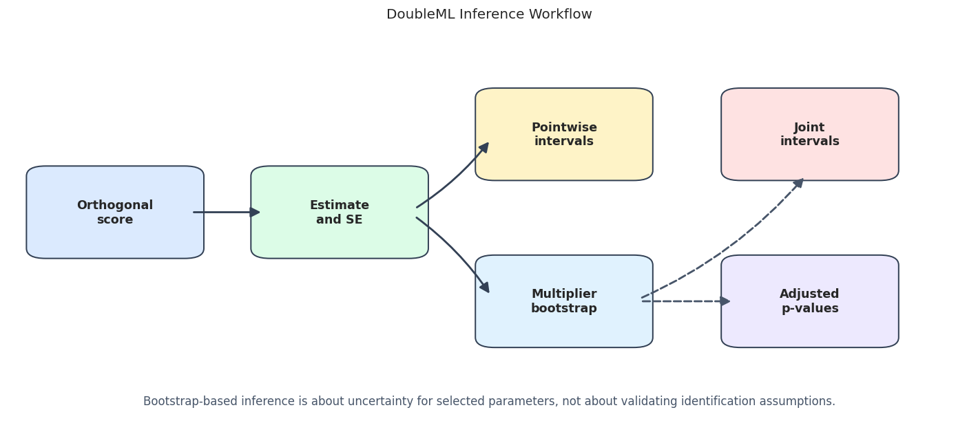
Inference Workflow Diagram

This diagram shows the inference stack. The point estimate and standard error come from the fitted orthogonal score. Bootstrap then approximates the distribution of score-based t-statistics, which supports joint intervals and Romano-Wolf-style p-value adjustment.

from matplotlib.patches import FancyArrowPatch, FancyBboxPatch

nodes = {
    "score": {"xy": (0.10, 0.58), "label": "Orthogonal\nscore", "color": "#dbeafe"},
    "estimate": {"xy": (0.31, 0.58), "label": "Estimate\nand SE", "color": "#dcfce7"},
    "pointwise": {"xy": (0.52, 0.72), "label": "Pointwise\nintervals", "color": "#fef3c7"},
    "bootstrap": {"xy": (0.52, 0.42), "label": "Multiplier\nbootstrap", "color": "#e0f2fe"},
    "joint": {"xy": (0.75, 0.72), "label": "Joint\nintervals", "color": "#fee2e2"},
    "adjust": {"xy": (0.75, 0.42), "label": "Adjusted\np-values", "color": "#ede9fe"},
}

fig, ax = plt.subplots(figsize=(12, 5.4))
ax.set_axis_off()
ax.set_xlim(0.0, 0.90)
ax.set_ylim(0.20, 0.90)
box_w, box_h = 0.13, 0.13


def anchor(name, side):
    x, y = nodes[name]["xy"]
    offsets = {"left": (-box_w / 2, 0), "right": (box_w / 2, 0), "top": (0, box_h / 2), "bottom": (0, -box_h / 2)}
    dx, dy = offsets[side]
    return (x + dx, y + dy)


def draw_arrow(start, end, color="#334155", style="solid", rad=0.0):
    arrow = FancyArrowPatch(
        start,
        end,
        arrowstyle="-|>",
        mutation_scale=18,
        linewidth=1.7,
        color=color,
        linestyle=style,
        connectionstyle=f"arc3,rad={rad}",
        shrinkA=8,
        shrinkB=8,
        zorder=5,
    )
    ax.add_patch(arrow)

for spec in nodes.values():
    x, y = spec["xy"]
    rect = FancyBboxPatch(
        (x - box_w / 2, y - box_h / 2),
        box_w,
        box_h,
        boxstyle="round,pad=0.018",
        facecolor=spec["color"],
        edgecolor="#334155",
        linewidth=1.2,
        zorder=3,
    )
    ax.add_patch(rect)
    ax.text(x, y, spec["label"], ha="center", va="center", fontsize=10.5, fontweight="bold", zorder=4)

draw_arrow(anchor("score", "right"), anchor("estimate", "left"))
draw_arrow(anchor("estimate", "right"), anchor("pointwise", "left"), rad=0.10)
draw_arrow(anchor("estimate", "right"), anchor("bootstrap", "left"), rad=-0.10)
draw_arrow(anchor("bootstrap", "right"), anchor("joint", "bottom"), color="#475569", style="dashed", rad=0.12)
draw_arrow(anchor("bootstrap", "right"), anchor("adjust", "left"), color="#475569", style="dashed")

ax.text(
    0.45,
    0.24,
    "Bootstrap-based inference is about uncertainty for selected parameters, not about validating identification assumptions.",
    ha="center",
    va="center",
    fontsize=10,
    color="#475569",
)
ax.set_title("DoubleML Inference Workflow", pad=14)
plt.tight_layout()
fig.savefig(FIGURE_DIR / f"{NOTEBOOK_PREFIX}_inference_workflow.png", bbox_inches="tight")
plt.show()

The workflow separates marginal inference from simultaneous inference. Both are useful, but they answer different questions.

Fit A Multi-Treatment DoubleMLPLR Model

We fit one PLR model with three treatment columns. DoubleML estimates one coefficient per treatment and returns a summary table with standard errors, t-statistics, p-values, and pointwise intervals.

The learner is a scaled RidgeCV pipeline. Scaling is inside the pipeline so preprocessing is done inside the cross-fitting folds rather than globally leaking information.

base_learner = Pipeline(
    [
        ("scale", StandardScaler()),
        ("model", RidgeCV(alphas=np.logspace(-3, 3, 15))),
    ]
)

dml_data = make_dml_data(inference_df)
inference_model = DoubleMLPLR(
    dml_data,
    ml_l=clone(base_learner),
    ml_m=clone(base_learner),
    n_folds=5,
    n_rep=3,
)

fit_start = time.perf_counter()
inference_model.fit()
fit_runtime = time.perf_counter() - fit_start

print(f"Fit runtime: {fit_runtime:.2f} seconds")
display(inference_model.summary)

Fit runtime: 0.27 seconds

	coef	std err	t	P>|t|	2.5 %	97.5 %
d_main	0.992578	0.034036	29.162472	5.804727e-187	0.925869	1.059288
d_secondary	0.462423	0.032758	14.116302	3.013958e-45	0.398219	0.526628
d_null	-0.016453	0.033438	-0.492045	6.226875e-01	-0.081989	0.049084

The summary table is the default inference view. It is pointwise: each row is interpreted as a separate treatment-effect estimate unless we add joint inference or p-value adjustment.

Standard Error And Pointwise Inference Table

This cell converts the DoubleML summary into an explicit reporting table and adds the known true effect from the simulation. In real data, the true effect column would not exist; it is included here only for learning.

standard_inference = inference_model.summary.reset_index().rename(columns={"index": "treatment"})
standard_inference["true_theta"] = standard_inference["treatment"].map(TRUE_THETAS)
standard_inference["bias_vs_true"] = standard_inference["coef"] - standard_inference["true_theta"]
standard_inference["covers_true_pointwise_95"] = (
    (standard_inference["2.5 %"] <= standard_inference["true_theta"])
    & (standard_inference["97.5 %"] >= standard_inference["true_theta"])
)

nuisance_rmse = inference_model.evaluate_learners(metric=rmse_metric)
nuisance_mae = inference_model.evaluate_learners(metric=mae_metric)
nuisance_quality = pd.DataFrame(
    [
        {
            "nuisance": name,
            "rmse_mean_across_treatments": float(np.nanmean(values)),
            "mae_mean_across_treatments": float(np.nanmean(nuisance_mae[name])),
        }
        for name, values in nuisance_rmse.items()
    ]
)

save_table(standard_inference, f"{NOTEBOOK_PREFIX}_standard_inference_summary.csv")
save_table(nuisance_quality, f"{NOTEBOOK_PREFIX}_nuisance_quality.csv")

display(standard_inference)
display(nuisance_quality)

	treatment	coef	std err	t	P>|t|	2.5 %	97.5 %	true_theta	bias_vs_true	covers_true_pointwise_95
0	d_main	0.992578	0.034036	29.162472	5.804727e-187	0.925869	1.059288	1.00	-0.007422	True
1	d_secondary	0.462423	0.032758	14.116302	3.013958e-45	0.398219	0.526628	0.45	0.012423	True
2	d_null	-0.016453	0.033438	-0.492045	6.226875e-01	-0.081989	0.049084	0.00	-0.016453	True

	nuisance	rmse_mean_across_treatments	mae_mean_across_treatments
0	ml_l	1.207413	0.960872
1	ml_m	1.004256	0.797188

The strong and moderate effects are clearly separated from zero, while the null effect is not. The nuisance-quality table records that inference was built from cross-fitted nuisance predictions rather than in-sample fits.

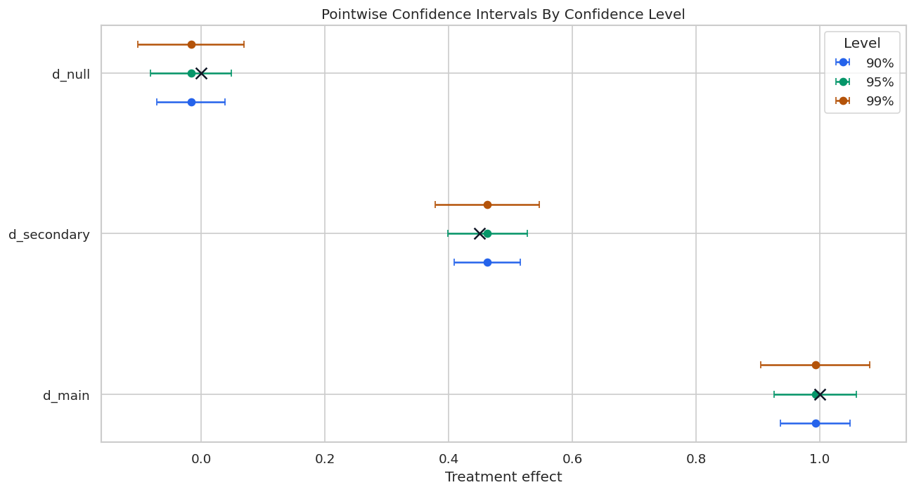
Confidence Levels And Interval Widths

Confidence intervals widen as the confidence level increases. This cell computes 90%, 95%, and 99% pointwise intervals manually from the coefficient and standard error.

ci_level_rows = []
for treatment, coef, se in zip(TREATMENT_COLS, inference_model.coef, inference_model.se):
    for level in [0.90, 0.95, 0.99]:
        lower, upper, critical_value = ci_from_coef_se(coef, se, level)
        ci_level_rows.append(
            {
                "treatment": treatment,
                "level": level,
                "critical_value": critical_value,
                "coef": coef,
                "se": se,
                "ci_lower": lower,
                "ci_upper": upper,
                "ci_width": upper - lower,
                "true_theta": TRUE_THETAS[treatment],
                "covers_true": lower <= TRUE_THETAS[treatment] <= upper,
            }
        )

ci_levels = pd.DataFrame(ci_level_rows)
save_table(ci_levels, f"{NOTEBOOK_PREFIX}_pointwise_confidence_levels.csv")
display(ci_levels)

	treatment	level	critical_value	coef	se	ci_lower	ci_upper	ci_width	true_theta	covers_true
0	d_main	0.90	1.644854	0.992578	0.034036	0.936594	1.048563	0.111969	1.00	True
1	d_main	0.95	1.959964	0.992578	0.034036	0.925869	1.059288	0.133419	1.00	True
2	d_main	0.99	2.575829	0.992578	0.034036	0.904907	1.080250	0.175343	1.00	True
3	d_secondary	0.90	1.644854	0.462423	0.032758	0.408541	0.516306	0.107765	0.45	True
4	d_secondary	0.95	1.959964	0.462423	0.032758	0.398219	0.526628	0.128409	0.45	True
5	d_secondary	0.99	2.575829	0.462423	0.032758	0.378044	0.546803	0.168759	0.45	True
6	d_null	0.90	1.644854	-0.016453	0.033438	-0.071453	0.038547	0.110000	0.00	True
7	d_null	0.95	1.959964	-0.016453	0.033438	-0.081989	0.049084	0.131073	0.00	True
8	d_null	0.99	2.575829	-0.016453	0.033438	-0.102582	0.069677	0.172259	0.00	True

The table shows the mechanical relationship between confidence level and interval width. Higher confidence requires a larger critical value, so the interval becomes wider.

Confidence Level Plot

The plot below shows the same idea visually. Each treatment receives three intervals, one per confidence level.

fig, ax = plt.subplots(figsize=(11, 6))
level_offsets = {0.90: -0.18, 0.95: 0.00, 0.99: 0.18}
y_positions = {treatment: idx for idx, treatment in enumerate(TREATMENT_COLS)}
colors = {0.90: "#2563eb", 0.95: "#059669", 0.99: "#b45309"}

for _, row in ci_levels.iterrows():
    y = y_positions[row["treatment"]] + level_offsets[row["level"]]
    ax.errorbar(
        x=row["coef"],
        y=y,
        xerr=[[row["coef"] - row["ci_lower"]], [row["ci_upper"] - row["coef"]]],
        fmt="o",
        color=colors[row["level"]],
        ecolor=colors[row["level"]],
        capsize=3,
        label=f"{int(row['level'] * 100)}%" if row["treatment"] == TREATMENT_COLS[0] else None,
    )

for treatment, true_value in TRUE_THETAS.items():
    ax.scatter(true_value, y_positions[treatment], marker="x", s=90, color="#111827", zorder=5)

ax.set_yticks(list(y_positions.values()))
ax.set_yticklabels(TREATMENT_COLS)
ax.set_title("Pointwise Confidence Intervals By Confidence Level")
ax.set_xlabel("Treatment effect")
ax.set_ylabel("")
ax.legend(title="Level", loc="best")
plt.tight_layout()
fig.savefig(FIGURE_DIR / f"{NOTEBOOK_PREFIX}_confidence_levels.png", bbox_inches="tight")
plt.show()

The x markers are the known true effects from the simulation. In applied work those markers do not exist, so the interval itself must be interpreted as an uncertainty statement under the design assumptions.

Multiplier Bootstrap

DoubleML’s bootstrap() method draws random multipliers for the estimated score contributions. This approximates the distribution of t-statistics without refitting all nuisance models for every bootstrap draw.

We use 800 bootstrap replications here. That is enough for a stable teaching plot while remaining fast.

np.random.seed(RANDOM_SEED)
bootstrap_start = time.perf_counter()
inference_model.bootstrap(method="normal", n_rep_boot=800)
bootstrap_runtime = time.perf_counter() - bootstrap_start

boot_stats = flatten_boot_t_stats(inference_model.boot_t_stat, TREATMENT_COLS)
boot_max_abs = (
    boot_stats.groupby(["boot_id", "rep_id"])["boot_t_stat"]
    .apply(lambda values: np.max(np.abs(values)))
    .reset_index(name="max_abs_t")
)
joint_critical_95 = boot_max_abs["max_abs_t"].quantile(0.95)

bootstrap_summary = pd.DataFrame(
    {
        "method": ["normal"],
        "n_rep_boot": [800],
        "bootstrap_runtime_seconds": [bootstrap_runtime],
        "joint_critical_95": [joint_critical_95],
    }
)

save_table(bootstrap_summary, f"{NOTEBOOK_PREFIX}_bootstrap_summary.csv")
save_table(boot_stats, f"{NOTEBOOK_PREFIX}_bootstrap_t_statistics.csv")
save_table(boot_max_abs, f"{NOTEBOOK_PREFIX}_bootstrap_max_abs_t.csv")

display(bootstrap_summary)
display(boot_stats.head())

	method	n_rep_boot	bootstrap_runtime_seconds	joint_critical_95
0	normal	800	0.039757	2.355717

	boot_id	treatment	rep_id	boot_t_stat
0	0	d_main	1	0.256778
1	0	d_main	2	1.507209
2	0	d_main	3	0.920467
3	0	d_secondary	1	-0.487059
4	0	d_secondary	2	0.921130

The bootstrap stores t-statistics for each treatment and each repeated sample split. The maximum absolute t-statistic distribution is what makes simultaneous inference wider than pointwise inference.

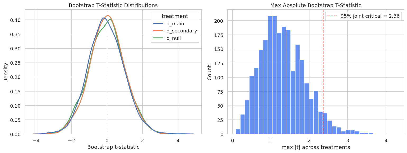
Bootstrap T-Statistic Distribution

This figure shows the bootstrap t-statistic distribution by treatment, plus the distribution of the maximum absolute t-statistic used for joint intervals.

fig, axes = plt.subplots(1, 2, figsize=(13, 5))

sns.kdeplot(
    data=boot_stats,
    x="boot_t_stat",
    hue="treatment",
    common_norm=False,
    linewidth=2,
    ax=axes[0],
)
axes[0].axvline(0, color="#111827", linestyle="--", linewidth=1.2)
axes[0].set_title("Bootstrap T-Statistic Distributions")
axes[0].set_xlabel("Bootstrap t-statistic")
axes[0].set_ylabel("Density")

sns.histplot(data=boot_max_abs, x="max_abs_t", bins=35, color="#2563eb", alpha=0.70, ax=axes[1])
axes[1].axvline(joint_critical_95, color="#dc2626", linestyle="--", linewidth=1.5, label=f"95% joint critical = {joint_critical_95:.2f}")
axes[1].set_title("Max Absolute Bootstrap T-Statistic")
axes[1].set_xlabel("max |t| across treatments")
axes[1].set_ylabel("Count")
axes[1].legend(loc="best")

plt.tight_layout()
fig.savefig(FIGURE_DIR / f"{NOTEBOOK_PREFIX}_bootstrap_t_distributions.png", bbox_inches="tight")
plt.show()

The max-statistic distribution has a larger critical value than the usual 1.96 pointwise normal cutoff. That is why joint intervals are wider.

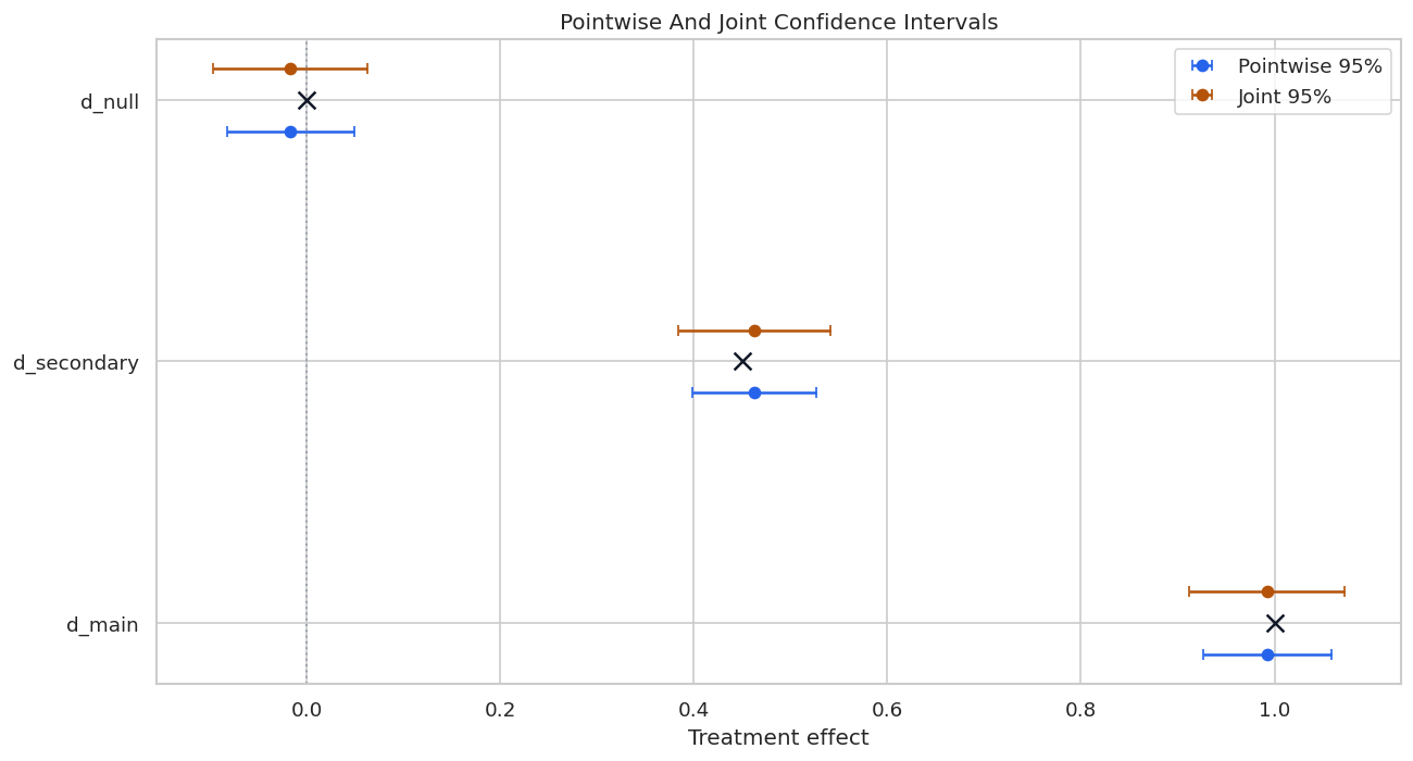
Pointwise Versus Joint Confidence Intervals

Now we compare pointwise 95% confidence intervals with bootstrap-based joint 95% confidence intervals. Joint intervals are appropriate when reporting several effects as a family and wanting simultaneous coverage.

pointwise_ci = inference_model.confint(joint=False, level=0.95).reset_index().rename(columns={"index": "treatment", "2.5 %": "pointwise_lower", "97.5 %": "pointwise_upper"})
joint_ci = inference_model.confint(joint=True, level=0.95).reset_index().rename(columns={"index": "treatment", "2.5 %": "joint_lower", "97.5 %": "joint_upper"})

ci_comparison = standard_inference[["treatment", "coef", "std err", "true_theta"]].merge(pointwise_ci, on="treatment").merge(joint_ci, on="treatment")
ci_comparison["pointwise_width"] = ci_comparison["pointwise_upper"] - ci_comparison["pointwise_lower"]
ci_comparison["joint_width"] = ci_comparison["joint_upper"] - ci_comparison["joint_lower"]
ci_comparison["joint_width_ratio"] = ci_comparison["joint_width"] / ci_comparison["pointwise_width"]
ci_comparison["pointwise_covers_true"] = (ci_comparison["pointwise_lower"] <= ci_comparison["true_theta"]) & (ci_comparison["pointwise_upper"] >= ci_comparison["true_theta"])
ci_comparison["joint_covers_true"] = (ci_comparison["joint_lower"] <= ci_comparison["true_theta"]) & (ci_comparison["joint_upper"] >= ci_comparison["true_theta"])

save_table(ci_comparison, f"{NOTEBOOK_PREFIX}_pointwise_vs_joint_ci.csv")
display(ci_comparison)

	treatment	coef	std err	true_theta	pointwise_lower	pointwise_upper	joint_lower	joint_upper	pointwise_width	joint_width	joint_width_ratio	pointwise_covers_true	joint_covers_true
0	d_main	0.992578	0.034036	1.00	0.925869	1.059288	0.912127	1.072009	0.133419	0.159882	1.198346	True	True
1	d_secondary	0.462423	0.032758	0.45	0.398219	0.526628	0.383856	0.540806	0.128409	0.156951	1.222269	True	True
2	d_null	-0.016453	0.033438	0.00	-0.081989	0.049084	-0.096650	0.063270	0.131073	0.159920	1.220085	True	True

The joint intervals are wider because they are calibrated to cover the collection of effects together. This is the right trade-off when the write-up makes simultaneous claims.

Pointwise Versus Joint Interval Plot

The plot below overlays the two interval types. Pointwise intervals are blue; joint intervals are orange. The black x marks the known true effect.

fig, ax = plt.subplots(figsize=(11, 6))
y_positions = {treatment: idx for idx, treatment in enumerate(TREATMENT_COLS)}

for _, row in ci_comparison.iterrows():
    y_base = y_positions[row["treatment"]]
    ax.errorbar(
        x=row["coef"],
        y=y_base - 0.12,
        xerr=[[row["coef"] - row["pointwise_lower"]], [row["pointwise_upper"] - row["coef"]]],
        fmt="o",
        color="#2563eb",
        ecolor="#2563eb",
        capsize=3,
        label="Pointwise 95%" if row["treatment"] == TREATMENT_COLS[0] else None,
    )
    ax.errorbar(
        x=row["coef"],
        y=y_base + 0.12,
        xerr=[[row["coef"] - row["joint_lower"]], [row["joint_upper"] - row["coef"]]],
        fmt="o",
        color="#b45309",
        ecolor="#b45309",
        capsize=3,
        label="Joint 95%" if row["treatment"] == TREATMENT_COLS[0] else None,
    )
    ax.scatter(row["true_theta"], y_base, marker="x", s=90, color="#111827", zorder=6)

ax.axvline(0, color="#9ca3af", linestyle=":", linewidth=1.2)
ax.set_yticks(list(y_positions.values()))
ax.set_yticklabels(TREATMENT_COLS)
ax.set_title("Pointwise And Joint Confidence Intervals")
ax.set_xlabel("Treatment effect")
ax.set_ylabel("")
ax.legend(loc="best")
plt.tight_layout()
fig.savefig(FIGURE_DIR / f"{NOTEBOOK_PREFIX}_pointwise_vs_joint_ci.png", bbox_inches="tight")
plt.show()

The null treatment interval includes zero under both approaches. The nonzero treatments remain clearly positive, even after joint calibration.

Bootstrap Method Comparison

DoubleML supports several multiplier bootstrap methods: normal, Bayes, and wild. In many well-behaved examples they give similar results, but comparing them is a useful robustness check.

bootstrap_method_rows = []
for method in ["normal", "Bayes", "wild"]:
    np.random.seed(RANDOM_SEED)
    inference_model.bootstrap(method=method, n_rep_boot=500)
    method_joint_ci = inference_model.confint(joint=True, level=0.95).reset_index().rename(columns={"index": "treatment", "2.5 %": "joint_lower", "97.5 %": "joint_upper"})
    method_joint_ci["method"] = method
    method_joint_ci["joint_width"] = method_joint_ci["joint_upper"] - method_joint_ci["joint_lower"]
    bootstrap_method_rows.append(method_joint_ci)

bootstrap_method_comparison = pd.concat(bootstrap_method_rows, ignore_index=True)
save_table(bootstrap_method_comparison, f"{NOTEBOOK_PREFIX}_bootstrap_method_comparison.csv")
display(bootstrap_method_comparison)

# Restore the normal bootstrap for the p-value adjustment sections below.
np.random.seed(RANDOM_SEED)
inference_model.bootstrap(method="normal", n_rep_boot=800)

	treatment	joint_lower	joint_upper	method	joint_width
0	d_main	0.913914	1.071688	normal	0.157774
1	d_secondary	0.385135	0.537902	normal	0.152767
2	d_null	-0.093496	0.060591	normal	0.154087
3	d_main	0.913589	1.072814	Bayes	0.159226
4	d_secondary	0.383071	0.538794	Bayes	0.155723
5	d_null	-0.097451	0.064545	Bayes	0.161996
6	d_main	0.914831	1.071966	wild	0.157136
7	d_secondary	0.383897	0.538196	wild	0.154299
8	d_null	-0.096607	0.063702	wild	0.160309

<doubleml.plm.plr.DoubleMLPLR at 0x7a08c517b620>

The methods produce similar joint intervals in this clean synthetic design. Bigger differences would be a signal to inspect sample size, score behavior, and model stability.

Multiple Testing Adjustment

When testing several effects, unadjusted p-values answer each test separately. Adjusted p-values account for the fact that several hypotheses are being examined. DoubleML supports Romano-Wolf adjustment through the bootstrap, and also methods such as Holm and Bonferroni through statsmodels.

romano_wolf = inference_model.p_adjust(method="romano-wolf").reset_index().rename(columns={"index": "treatment", "pval": "romano_wolf_pval"})
holm = inference_model.p_adjust(method="holm").reset_index().rename(columns={"index": "treatment", "pval": "holm_pval"})
bonferroni = inference_model.p_adjust(method="bonferroni").reset_index().rename(columns={"index": "treatment", "pval": "bonferroni_pval"})

pvalue_comparison = standard_inference[["treatment", "coef", "P>|t|", "true_theta"]].rename(columns={"P>|t|": "pointwise_pval"})
pvalue_comparison = pvalue_comparison.merge(romano_wolf[["treatment", "romano_wolf_pval"]], on="treatment")
pvalue_comparison = pvalue_comparison.merge(holm[["treatment", "holm_pval"]], on="treatment")
pvalue_comparison = pvalue_comparison.merge(bonferroni[["treatment", "bonferroni_pval"]], on="treatment")

save_table(pvalue_comparison, f"{NOTEBOOK_PREFIX}_adjusted_pvalue_comparison.csv")
display(pvalue_comparison)

	treatment	coef	pointwise_pval	true_theta	romano_wolf_pval	holm_pval	bonferroni_pval
0	d_main	0.992578	5.804727e-187	1.00	0.00000	0.000000	0.0
1	d_secondary	0.462423	3.013958e-45	0.45	0.00000	0.000000	0.0
2	d_null	-0.016453	6.226875e-01	0.00	0.61375	0.622688	1.0

The two true nonzero effects remain significant after adjustment, while the null treatment remains non-significant. That is the behavior we hope to see in this teaching simulation.

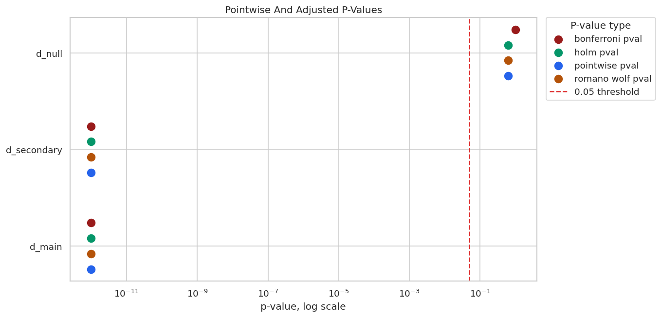
Adjusted P-Value Plot

The plot below shows pointwise and adjusted p-values on a log scale. The dashed line marks 0.05.

pvalue_plot = pvalue_comparison.melt(
    id_vars="treatment",
    value_vars=["pointwise_pval", "romano_wolf_pval", "holm_pval", "bonferroni_pval"],
    var_name="pvalue_type",
    value_name="pvalue",
)
pvalue_plot["pvalue_for_plot"] = pvalue_plot["pvalue"].clip(lower=1e-12)

pvalue_offsets = {
    "pointwise_pval": -0.24,
    "romano_wolf_pval": -0.08,
    "holm_pval": 0.08,
    "bonferroni_pval": 0.24,
}
pvalue_colors = {
    "pointwise_pval": "#2563eb",
    "romano_wolf_pval": "#b45309",
    "holm_pval": "#059669",
    "bonferroni_pval": "#991b1b",
}
y_positions = {treatment: idx for idx, treatment in enumerate(TREATMENT_COLS)}

fig, ax = plt.subplots(figsize=(11.5, 5.6))
for pvalue_type, group in pvalue_plot.groupby("pvalue_type"):
    ax.scatter(
        group["pvalue_for_plot"],
        [y_positions[treatment] + pvalue_offsets[pvalue_type] for treatment in group["treatment"]],
        s=90,
        color=pvalue_colors[pvalue_type],
        label=pvalue_type.replace("_", " "),
    )

ax.axvline(0.05, color="#dc2626", linestyle="--", linewidth=1.5, label="0.05 threshold")
ax.set_xscale("log")
ax.set_yticks(list(y_positions.values()))
ax.set_yticklabels(TREATMENT_COLS)
ax.set_title("Pointwise And Adjusted P-Values")
ax.set_xlabel("p-value, log scale")
ax.set_ylabel("")
ax.legend(title="P-value type", bbox_to_anchor=(1.02, 1), loc="upper left", borderaxespad=0)
plt.tight_layout()
fig.savefig(FIGURE_DIR / f"{NOTEBOOK_PREFIX}_adjusted_pvalues.png", bbox_inches="tight")
plt.show()

The log scale makes tiny p-values visible while still showing the null treatment near the non-significant region. Adjustment matters most when there are several borderline effects.

Small Coverage Simulation

This short simulation repeats a simple single-treatment PLR design several times and checks whether the pointwise 95% confidence interval covers the known true effect. It is intentionally small and should be read as a teaching sketch, not a formal Monte Carlo study.

A real simulation study would use many more repetitions, multiple sample sizes, and a fixed analysis plan.

def simulate_single_effect_dataset(seed, n_obs=350, n_controls=8, true_theta=0.80):
    rng_local = np.random.default_rng(seed)
    x = rng_local.normal(size=(n_obs, n_controls))
    df = pd.DataFrame(x, columns=[f"x{i}" for i in range(n_controls)])
    treatment_nuisance = 0.50 * df["x0"] - 0.30 * df["x1"] + 0.25 * df["x2"]
    outcome_nuisance = 0.60 * df["x0"] + 0.35 * df["x3"] - 0.25 * df["x4"]
    df["treatment"] = treatment_nuisance + rng_local.normal(size=n_obs)
    df["outcome"] = true_theta * df["treatment"] + outcome_nuisance + rng_local.normal(size=n_obs)
    return df

coverage_rows = []
coverage_true_theta = 0.80
coverage_learner = Ridge(alpha=1.0)

for sim_id in range(30):
    sim_df = simulate_single_effect_dataset(seed=1_000 + sim_id, true_theta=coverage_true_theta)
    sim_data = DoubleMLData(sim_df, y_col="outcome", d_cols="treatment")
    sim_model = DoubleMLPLR(
        sim_data,
        ml_l=clone(coverage_learner),
        ml_m=clone(coverage_learner),
        n_folds=3,
    )
    sim_model.fit()
    sim_ci = sim_model.confint(level=0.95).iloc[0]
    coverage_rows.append(
        {
            "sim_id": sim_id,
            "theta_hat": float(sim_model.coef[0]),
            "se": float(sim_model.se[0]),
            "ci_lower": float(sim_ci.iloc[0]),
            "ci_upper": float(sim_ci.iloc[1]),
            "ci_width": float(sim_ci.iloc[1] - sim_ci.iloc[0]),
            "covers_true": bool(sim_ci.iloc[0] <= coverage_true_theta <= sim_ci.iloc[1]),
        }
    )

coverage_simulation = pd.DataFrame(coverage_rows)
coverage_summary = pd.DataFrame(
    {
        "n_simulations": [len(coverage_simulation)],
        "true_theta": [coverage_true_theta],
        "coverage_rate": [coverage_simulation["covers_true"].mean()],
        "mean_theta_hat": [coverage_simulation["theta_hat"].mean()],
        "sd_theta_hat": [coverage_simulation["theta_hat"].std()],
        "mean_reported_se": [coverage_simulation["se"].mean()],
        "mean_ci_width": [coverage_simulation["ci_width"].mean()],
    }
)

save_table(coverage_simulation, f"{NOTEBOOK_PREFIX}_coverage_simulation.csv")
save_table(coverage_summary, f"{NOTEBOOK_PREFIX}_coverage_summary.csv")

display(coverage_summary)
display(coverage_simulation.head())

	n_simulations	true_theta	coverage_rate	mean_theta_hat	sd_theta_hat	mean_reported_se	mean_ci_width
0	30	0.8	1.0	0.812886	0.04525	0.052825	0.207069

	sim_id	theta_hat	se	ci_lower	ci_upper	ci_width	covers_true
0	0	0.884287	0.043571	0.798890	0.969685	0.170795	True
1	1	0.774099	0.045587	0.684750	0.863447	0.178698	True
2	2	0.755067	0.055617	0.646060	0.864073	0.218013	True
3	3	0.860735	0.052665	0.757514	0.963956	0.206442	True
4	4	0.803388	0.051312	0.702819	0.903958	0.201139	True

The empirical coverage rate will not be exactly 95% with only 30 simulations. The point is to connect the interval formula to repeated-sampling behavior: over many hypothetical datasets, valid 95% intervals should cover the true effect about 95% of the time.

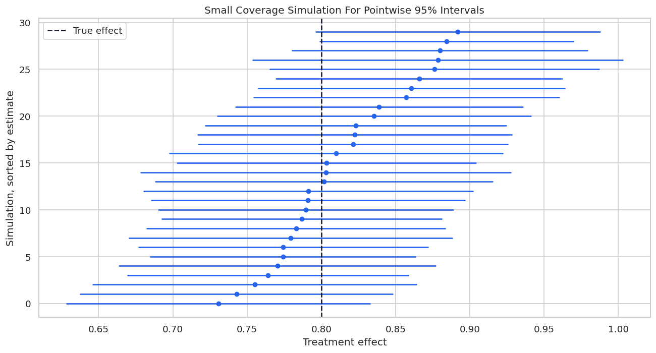
Coverage Simulation Plot

Each horizontal line is one simulated 95% confidence interval. Blue intervals cover the true effect; red intervals miss it.

plot_coverage = coverage_simulation.sort_values("theta_hat").reset_index(drop=True)
plot_coverage["ordered_sim"] = np.arange(len(plot_coverage))
plot_coverage["coverage_label"] = np.where(plot_coverage["covers_true"], "covers", "misses")

fig, ax = plt.subplots(figsize=(11, 6))
for _, row in plot_coverage.iterrows():
    color = "#2563eb" if row["covers_true"] else "#dc2626"
    ax.plot([row["ci_lower"], row["ci_upper"]], [row["ordered_sim"], row["ordered_sim"]], color=color, linewidth=1.6)
    ax.scatter(row["theta_hat"], row["ordered_sim"], color=color, s=24)
ax.axvline(coverage_true_theta, color="#111827", linestyle="--", linewidth=1.5, label="True effect")
ax.set_title("Small Coverage Simulation For Pointwise 95% Intervals")
ax.set_xlabel("Treatment effect")
ax.set_ylabel("Simulation, sorted by estimate")
ax.legend(loc="best")
plt.tight_layout()
fig.savefig(FIGURE_DIR / f"{NOTEBOOK_PREFIX}_coverage_simulation.png", bbox_inches="tight")
plt.show()

Coverage is a repeated-sampling idea. A single applied interval either contains the true effect or it does not, but we never observe that directly. The simulation is here to make the concept concrete.

Reporting Checklist

This checklist summarizes what should be reported when presenting DoubleML inference results. The emphasis is on clarity: point estimate, uncertainty type, bootstrap settings, and multiple-testing choices should all be visible.

inference_reporting_checklist = pd.DataFrame(
    [
        {"item": "State the estimand and treatment columns", "why": "Inference is only meaningful after the target is clear."},
        {"item": "Report coefficient, standard error, and confidence interval", "why": "A point estimate without uncertainty is incomplete."},
        {"item": "Say whether intervals are pointwise or joint", "why": "These intervals answer different reporting questions."},
        {"item": "Document bootstrap method and number of replications", "why": "Joint intervals and Romano-Wolf adjustment depend on bootstrap settings."},
        {"item": "Use adjusted p-values for multiple treatment tests", "why": "Several tests increase the chance of false discoveries."},
        {"item": "Report nuisance model and cross-fitting choices", "why": "Uncertainty is conditional on the fitted DoubleML design."},
        {"item": "Separate statistical uncertainty from identification uncertainty", "why": "Bootstrap cannot fix omitted variables, bad timing, or invalid instruments."},
    ]
)

save_table(inference_reporting_checklist, f"{NOTEBOOK_PREFIX}_inference_reporting_checklist.csv")
display(inference_reporting_checklist)

	item	why
0	State the estimand and treatment columns	Inference is only meaningful after the target ...
1	Report coefficient, standard error, and confid...	A point estimate without uncertainty is incomp...
2	Say whether intervals are pointwise or joint	These intervals answer different reporting que...
3	Document bootstrap method and number of replic...	Joint intervals and Romano-Wolf adjustment dep...
4	Use adjusted p-values for multiple treatment t...	Several tests increase the chance of false dis...
5	Report nuisance model and cross-fitting choices	Uncertainty is conditional on the fitted Doubl...
6	Separate statistical uncertainty from identifi...	Bootstrap cannot fix omitted variables, bad ti...

The last row is the most important. Statistical inference quantifies sampling uncertainty under the design; it does not prove the design is correct.

Report Template And Artifact Manifest

The final cell writes a report template and an artifact manifest. This keeps the tutorial reproducible and gives a structure for future applied analyses.

report_text = f"""
# DoubleML Inference Report Template

## Estimand And Model
- Outcome:
- Treatment column(s):
- Control set:
- DoubleML model class:
- Nuisance learners:
- Cross-fitting design:

## Point Estimates
- Coefficient table:
- Standard errors:
- Pointwise confidence intervals:

## Bootstrap And Simultaneous Inference
- Bootstrap method:
- Bootstrap replications:
- Joint confidence intervals:
- Adjusted p-value method:

## Main Findings
- Effects clearly separated from zero:
- Effects sensitive to adjustment:
- Null or inconclusive effects:

## Caveats
- Identification assumptions:
- Sample size and split stability:
- Multiple testing:
- Remaining uncertainty not captured by standard errors:
""".strip()

report_path = REPORT_DIR / f"{NOTEBOOK_PREFIX}_inference_report_template.md"
report_path.write_text(report_text)

artifact_manifest = pd.DataFrame(
    [
        {"artifact": "synthetic multi-treatment PLR data", "path": str(DATASET_DIR / f"{NOTEBOOK_PREFIX}_synthetic_multitreatment_plr_data.csv")},
        {"artifact": "standard inference summary", "path": str(TABLE_DIR / f"{NOTEBOOK_PREFIX}_standard_inference_summary.csv")},
        {"artifact": "pointwise vs joint intervals", "path": str(TABLE_DIR / f"{NOTEBOOK_PREFIX}_pointwise_vs_joint_ci.csv")},
        {"artifact": "adjusted p-value comparison", "path": str(TABLE_DIR / f"{NOTEBOOK_PREFIX}_adjusted_pvalue_comparison.csv")},
        {"artifact": "coverage simulation", "path": str(TABLE_DIR / f"{NOTEBOOK_PREFIX}_coverage_simulation.csv")},
        {"artifact": "report template", "path": str(report_path)},
        {"artifact": "inference workflow figure", "path": str(FIGURE_DIR / f"{NOTEBOOK_PREFIX}_inference_workflow.png")},
        {"artifact": "pointwise vs joint interval figure", "path": str(FIGURE_DIR / f"{NOTEBOOK_PREFIX}_pointwise_vs_joint_ci.png")},
    ]
)

save_table(artifact_manifest, f"{NOTEBOOK_PREFIX}_artifact_manifest.csv")
display(Markdown(f"Report template written to `{report_path}`"))
display(artifact_manifest)

Report template written to /home/apex/Documents/ranking_sys/notebooks/tutorials/doubleml/outputs/reports/12_inference_report_template.md

	artifact	path
0	synthetic multi-treatment PLR data	/home/apex/Documents/ranking_sys/notebooks/tut...
1	standard inference summary	/home/apex/Documents/ranking_sys/notebooks/tut...
2	pointwise vs joint intervals	/home/apex/Documents/ranking_sys/notebooks/tut...
3	adjusted p-value comparison	/home/apex/Documents/ranking_sys/notebooks/tut...
4	coverage simulation	/home/apex/Documents/ranking_sys/notebooks/tut...
5	report template	/home/apex/Documents/ranking_sys/notebooks/tut...
6	inference workflow figure	/home/apex/Documents/ranking_sys/notebooks/tut...
7	pointwise vs joint interval figure	/home/apex/Documents/ranking_sys/notebooks/tut...

The notebook now covers the core DoubleML inference workflow: standard errors, pointwise intervals, multiplier bootstrap, joint intervals, adjusted p-values, and reporting discipline.

What Comes Next

The next natural topic is sensitivity analysis for unobserved confounding: how DoubleML represents robustness to omitted confounders and how to explain those sensitivity parameters in a way that is useful rather than mystical.