DoubleML Tutorial 11: Sample Splitting, Cross-Fitting, And Repeated Cross-Fitting

This notebook is about the machinery that makes double machine learning more than “fit a flexible model and regress residuals.” The key idea is cross-fitting: nuisance models are trained on one part of the data and used to predict nuisance quantities on held-out rows. Those held-out nuisance predictions are then used inside an orthogonal score for the treatment effect.

Why does this matter?

Flexible learners can overfit. If a nuisance model predicts the same rows it was trained on, the residuals can become artificially small or distorted. In ordinary prediction work, that is a validation problem. In causal estimation, it is worse: distorted residuals can distort the orthogonal score itself.

A PLR score can be written informally as residualizing both outcome and treatment:

\[ \tilde{Y}_i = Y_i - \hat{\ell}(X_i), \quad \tilde{D}_i = D_i - \hat{m}(X_i), \]

and then estimating the treatment effect from the relationship between (_i) and (_i). Cross-fitting asks for ((X_i)) and ((X_i)) to be predictions from models that did not train on row (i).

This notebook covers five practical topics:

1. What K-fold cross-fitting is doing.
2. How fold count changes training/validation trade-offs.
3. How repeated cross-fitting reduces dependence on one random split.
4. How to set external splits for grouped data.
5. Why in-sample nuisance residualization can fail with very flexible learners.

Expected runtime: about 30-60 seconds on a laptop. The notebook fits several DoubleML models and a few manual cross-fitting models, but all learners are configured to stay tutorial-friendly.

Setup

The setup cell follows the same pattern as the earlier DoubleML tutorials. It creates output folders, sets a local Matplotlib cache, imports DoubleML and sklearn tools, and fixes global plotting defaults.

from pathlib import Path
import os
import time
import warnings

PROJECT_ROOT = Path.cwd().resolve()
if PROJECT_ROOT.name == "doubleml":
    PROJECT_ROOT = PROJECT_ROOT.parents[2]

OUTPUT_DIR = PROJECT_ROOT / "notebooks" / "tutorials" / "doubleml" / "outputs"
DATASET_DIR = OUTPUT_DIR / "datasets"
FIGURE_DIR = OUTPUT_DIR / "figures"
TABLE_DIR = OUTPUT_DIR / "tables"
REPORT_DIR = OUTPUT_DIR / "reports"
MATPLOTLIB_CACHE_DIR = OUTPUT_DIR / "matplotlib_cache"

for directory in [DATASET_DIR, FIGURE_DIR, TABLE_DIR, REPORT_DIR, MATPLOTLIB_CACHE_DIR]:
    directory.mkdir(parents=True, exist_ok=True)

os.environ.setdefault("MPLCONFIGDIR", str(MATPLOTLIB_CACHE_DIR))
warnings.filterwarnings("ignore", category=FutureWarning)
warnings.filterwarnings("ignore", message="X does not have valid feature names.*")
warnings.filterwarnings("ignore", message="IProgress not found.*")

import numpy as np
import pandas as pd
import matplotlib.pyplot as plt
import seaborn as sns
from IPython.display import Markdown, display

import doubleml as dml
from doubleml import DoubleMLData, DoubleMLPLR

from sklearn.base import clone
from sklearn.ensemble import ExtraTreesRegressor, HistGradientBoostingRegressor
from sklearn.linear_model import LinearRegression
from sklearn.metrics import mean_absolute_error, mean_squared_error, r2_score
from sklearn.model_selection import GroupKFold, KFold

NOTEBOOK_PREFIX = "11"
RANDOM_SEED = 42
TRUE_THETA = 1.00

sns.set_theme(style="whitegrid", context="notebook")
plt.rcParams.update({"figure.dpi": 120, "savefig.dpi": 160})

print(f"DoubleML version: {dml.__version__}")
print(f"Output directory: {OUTPUT_DIR}")

DoubleML version: 0.11.2
Output directory: /home/apex/Documents/ranking_sys/notebooks/tutorials/doubleml/outputs

The setup output confirms the package version and the artifact location. The notebook uses only local synthetic data, so every result should be reproducible from the cells below.

Helper Functions

These helpers handle repeated notebook chores: saving tables, building DoubleMLData, computing nuisance metrics, creating sample splits, and fitting a PLR model with a specified split design.

The most important helper is fit_plr_with_splits(). It lets us compare DoubleML models while controlling whether the sample splitting is drawn internally or provided externally.

def save_table(df, filename):
    path = TABLE_DIR / filename
    df.to_csv(path, index=False)
    return path


def save_dataset(df, filename):
    path = DATASET_DIR / filename
    df.to_csv(path, index=False)
    return path


def rmse_metric(y_true, y_pred):
    mask = ~np.isnan(y_true)
    return mean_squared_error(y_true[mask], y_pred[mask]) ** 0.5


def mae_metric(y_true, y_pred):
    mask = ~np.isnan(y_true)
    return mean_absolute_error(y_true[mask], y_pred[mask])


def model_x_cols(df):
    excluded = {"unit_id", "user_id", "outcome", "treatment", "true_g", "true_m", "user_effect"}
    return [col for col in df.columns if col not in excluded]


def make_plr_data(df):
    return DoubleMLData(df, y_col="outcome", d_cols="treatment", x_cols=model_x_cols(df))


def make_kfold_splits(df, n_folds, seed):
    splitter = KFold(n_splits=n_folds, shuffle=True, random_state=seed)
    return list(splitter.split(df))


def make_repeated_kfold_splits(df, n_folds, n_rep, seed):
    return [make_kfold_splits(df, n_folds=n_folds, seed=seed + rep) for rep in range(n_rep)]


def fit_plr_with_splits(df, learner, label, n_folds=5, n_rep=1, all_smpls=None, seed=RANDOM_SEED):
    dml_data = make_plr_data(df)
    plr = DoubleMLPLR(
        dml_data,
        ml_l=clone(learner),
        ml_m=clone(learner),
        n_folds=n_folds,
        n_rep=n_rep,
        draw_sample_splitting=all_smpls is None,
    )
    if all_smpls is not None:
        plr.set_sample_splitting(all_smpls)

    start = time.perf_counter()
    plr.fit()
    runtime_seconds = time.perf_counter() - start

    rmse = plr.evaluate_learners(metric=rmse_metric)
    mae = plr.evaluate_learners(metric=mae_metric)

    row = {
        "label": label,
        "n_folds": n_folds,
        "n_rep": n_rep,
        "theta_hat": float(plr.coef[0]),
        "se": float(plr.se[0]),
        "ci_95_lower": float(plr.confint().iloc[0, 0]),
        "ci_95_upper": float(plr.confint().iloc[0, 1]),
        "bias_vs_true": float(plr.coef[0] - TRUE_THETA),
        "abs_bias_vs_true": float(abs(plr.coef[0] - TRUE_THETA)),
        "rmse_ml_l": float(rmse["ml_l"][0, 0]),
        "rmse_ml_m": float(rmse["ml_m"][0, 0]),
        "mae_ml_l": float(mae["ml_l"][0, 0]),
        "mae_ml_m": float(mae["ml_m"][0, 0]),
        "runtime_seconds": runtime_seconds,
    }
    return plr, row


def fold_assignment_frame(all_smpls, n_obs, n_rep_to_show=1):
    rows = []
    for rep_id, rep_splits in enumerate(all_smpls[:n_rep_to_show], start=1):
        assignment = np.full(n_obs, -1)
        for fold_id, (_, test_idx) in enumerate(rep_splits, start=1):
            assignment[test_idx] = fold_id
        for row_id, fold_id in enumerate(assignment):
            rows.append({"rep": rep_id, "row_id": row_id, "fold": fold_id})
    return pd.DataFrame(rows)


def group_overlap_audit(df, splits, group_col="user_id"):
    rows = []
    for fold_id, (train_idx, test_idx) in enumerate(splits, start=1):
        train_groups = set(df.iloc[train_idx][group_col])
        test_groups = set(df.iloc[test_idx][group_col])
        overlap = train_groups.intersection(test_groups)
        rows.append(
            {
                "fold": fold_id,
                "train_rows": len(train_idx),
                "test_rows": len(test_idx),
                "train_groups": len(train_groups),
                "test_groups": len(test_groups),
                "overlap_groups": len(overlap),
            }
        )
    return pd.DataFrame(rows)

The helpers make the split structure explicit. A DoubleML repeated split is represented as a list of repetitions, where each repetition is itself a list of train/test index pairs.

Split Vocabulary

This table defines the terms used throughout the notebook. The distinction between sample splitting, cross-fitting, and repeated cross-fitting is subtle but important.

split_vocabulary = pd.DataFrame(
    [
        {
            "term": "Sample splitting",
            "meaning": "Partition rows into training and held-out pieces for nuisance prediction.",
            "why it matters": "Prevents nuisance predictions for a row from being trained on that same row.",
        },
        {
            "term": "K-fold cross-fitting",
            "meaning": "Split data into K folds; train nuisances on K-1 folds and predict the held-out fold, repeated for every fold.",
            "why it matters": "Every row gets an out-of-fold nuisance prediction while still using most data for training.",
        },
        {
            "term": "Repeated cross-fitting",
            "meaning": "Draw multiple K-fold splits and aggregate the resulting DoubleML estimates.",
            "why it matters": "Reduces dependence on one random partition of the sample.",
        },
        {
            "term": "External sample splits",
            "meaning": "User-supplied train/test fold indices passed into DoubleML.",
            "why it matters": "Needed for grouped, temporal, clustered, or otherwise constrained validation designs.",
        },
        {
            "term": "In-sample residualization",
            "meaning": "Fit nuisances and predict on the same rows used for fitting.",
            "why it matters": "Can badly distort residuals with flexible learners; useful here only as a cautionary comparison.",
        },
    ]
)

save_table(split_vocabulary, f"{NOTEBOOK_PREFIX}_split_vocabulary.csv")
display(split_vocabulary)

	term	meaning	why it matters
0	Sample splitting	Partition rows into training and held-out piec...	Prevents nuisance predictions for a row from b...
1	K-fold cross-fitting	Split data into K folds; train nuisances on K-...	Every row gets an out-of-fold nuisance predict...
2	Repeated cross-fitting	Draw multiple K-fold splits and aggregate the ...	Reduces dependence on one random partition of ...
3	External sample splits	User-supplied train/test fold indices passed i...	Needed for grouped, temporal, clustered, or ot...
4	In-sample residualization	Fit nuisances and predict on the same rows use...	Can badly distort residuals with flexible lear...

The vocabulary separates concepts that often get compressed into one phrase. DoubleML automates a lot of this, but the analyst still needs to know what split design is being used.

Synthetic Panel-Like PLR Data

We simulate a small panel-like dataset with repeated observations per user. The user identifier is excluded from the model controls, but a noisy user-level proxy is included. This lets us demonstrate both ordinary random folds and group-aware external folds.

The true treatment effect is TRUE_THETA = 1.00. The treatment and outcome both depend on nonlinear functions of observed controls, so cross-fitting with a nonlinear learner is useful.

rng = np.random.default_rng(RANDOM_SEED)

n_users = 240
observations_per_user = 4
n_obs = n_users * observations_per_user
n_features = 10

user_id = np.repeat(np.arange(n_users), observations_per_user)
user_effect = rng.normal(size=n_users)
feature_array = rng.normal(size=(n_obs, n_features))

plr_df = pd.DataFrame(feature_array, columns=[f"x{i:02d}" for i in range(n_features)])
plr_df.insert(0, "unit_id", np.arange(n_obs))
plr_df["user_id"] = user_id
plr_df["user_effect"] = np.repeat(user_effect, observations_per_user)
plr_df["user_effect_proxy"] = plr_df["user_effect"] + 0.30 * rng.normal(size=n_obs)

plr_df["true_m"] = (
    0.50 * np.sin(plr_df["x00"])
    + 0.35 * plr_df["x01"] ** 2
    - 0.35 * plr_df["x02"]
    + 0.35 * plr_df["user_effect_proxy"]
    + 0.25 * plr_df["x03"] * plr_df["x04"]
)
plr_df["true_g"] = (
    0.80 * np.cos(plr_df["x00"])
    + 0.35 * plr_df["x05"] * plr_df["x06"]
    + 0.35 * plr_df["user_effect_proxy"]
    + 0.20 * plr_df["x07"] ** 2
)

plr_df["treatment"] = plr_df["true_m"] + rng.normal(scale=1.00, size=n_obs)
plr_df["outcome"] = TRUE_THETA * plr_df["treatment"] + plr_df["true_g"] + rng.normal(scale=1.00, size=n_obs)

save_dataset(plr_df, f"{NOTEBOOK_PREFIX}_synthetic_panel_like_plr_data.csv")
plr_df.head()

	unit_id	x00	x01	x02	x03	x04	x05	x06	x07	x08	x09	user_id	user_effect	user_effect_proxy	true_m	true_g	treatment	outcome
0	0	-0.876861	-0.094263	-1.757728	-1.467045	2.129247	-1.287423	-1.096786	1.836914	2.905067	-1.171567	0	0.304717	0.234338	-0.464960	1.762732	-0.438308	2.294601
1	1	-0.368249	0.341556	1.728698	-0.986857	-0.245278	0.777338	0.434766	-0.376156	-0.133823	-1.374896	0	0.304717	0.229064	-0.603518	0.973124	-1.159085	-0.983254
2	2	-0.238174	-0.266387	0.232170	-0.555327	0.471539	1.012716	0.155429	0.351756	0.053155	0.000084	0	0.304717	-0.211527	-0.313886	0.783220	-0.831732	-0.594069
3	3	-0.721558	0.316494	-0.097287	2.093168	1.573355	0.385847	-0.763057	-1.112411	1.191143	0.262749	0	0.304717	0.466637	0.725479	0.908389	0.162252	0.081954
4	4	0.480143	-1.744586	0.927438	0.454420	-1.110431	-0.471525	0.263717	0.052467	-0.292171	-0.103488	1	-1.039984	-1.248753	0.408389	0.229508	-0.065415	-0.492320

The first rows show a dataset with repeated users and known oracle nuisance functions. The oracle columns help us evaluate the simulation but are excluded from the DoubleML controls.

Data Audit

The audit records the sample size, number of groups, missingness, and the strength of confounding. A split tutorial still needs a design audit: cross-fitting helps with overfitting, not with a wrong treatment definition or missing confounders.

field_dictionary = pd.DataFrame(
    [
        {"column": "unit_id", "role": "identifier", "description": "Synthetic row identifier; excluded from modeling."},
        {"column": "user_id", "role": "group identifier", "description": "Repeated-observation group id; used only for external GroupKFold splits."},
        {"column": "x00-x09", "role": "observed controls", "description": "Numeric pre-treatment controls."},
        {"column": "user_effect_proxy", "role": "observed control", "description": "Noisy pre-treatment proxy for user-level heterogeneity."},
        {"column": "user_effect", "role": "oracle only", "description": "Latent user effect used only in simulation diagnostics."},
        {"column": "true_m", "role": "oracle only", "description": "True treatment nuisance E[D|X] used only for simulation diagnostics."},
        {"column": "true_g", "role": "oracle only", "description": "True outcome nuisance component g0(X) used only for simulation diagnostics."},
        {"column": "treatment", "role": "treatment", "description": "Continuous treatment D."},
        {"column": "outcome", "role": "outcome", "description": "Continuous outcome Y."},
    ]
)

data_audit = pd.DataFrame(
    {
        "n_rows": [len(plr_df)],
        "n_users": [plr_df["user_id"].nunique()],
        "observations_per_user": [observations_per_user],
        "model_controls": [len(model_x_cols(plr_df))],
        "missing_cells": [int(plr_df.isna().sum().sum())],
        "true_theta": [TRUE_THETA],
        "corr_treatment_true_m": [plr_df["treatment"].corr(plr_df["true_m"])],
        "corr_treatment_true_g": [plr_df["treatment"].corr(plr_df["true_g"])],
    }
)

save_table(field_dictionary, f"{NOTEBOOK_PREFIX}_field_dictionary.csv")
save_table(data_audit, f"{NOTEBOOK_PREFIX}_data_audit.csv")

display(field_dictionary)
display(data_audit)

	column	role	description
0	unit_id	identifier	Synthetic row identifier; excluded from modeling.
1	user_id	group identifier	Repeated-observation group id; used only for e...
2	x00-x09	observed controls	Numeric pre-treatment controls.
3	user_effect_proxy	observed control	Noisy pre-treatment proxy for user-level heter...
4	user_effect	oracle only	Latent user effect used only in simulation dia...
5	true_m	oracle only	True treatment nuisance E[D|X] used only for s...
6	true_g	oracle only	True outcome nuisance component g0(X) used onl...
7	treatment	treatment	Continuous treatment D.
8	outcome	outcome	Continuous outcome Y.

	n_rows	n_users	observations_per_user	model_controls	missing_cells	true_theta	corr_treatment_true_m	corr_treatment_true_g
0	960	240	4	11	0	1.0	0.649431	0.1303

The treatment is related to both the treatment nuisance and outcome-relevant control structure. That is the confounding pattern the PLR score is designed to address.

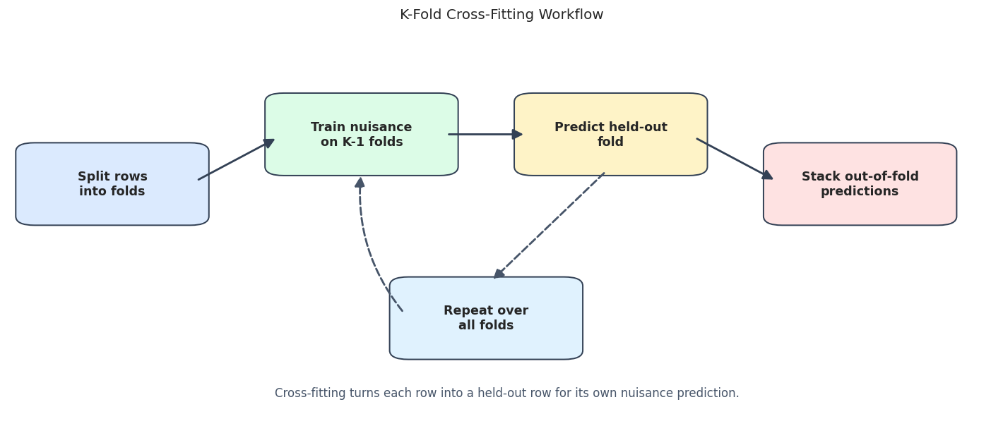
Cross-Fitting Design Diagram

The diagram below shows why a row’s nuisance prediction is out-of-fold. A fold’s held-out rows are predicted by a model trained on the other folds. After all folds are predicted, DoubleML has one out-of-fold nuisance prediction per row.

from matplotlib.patches import FancyArrowPatch, FancyBboxPatch

nodes = {
    "split": {"xy": (0.10, 0.62), "label": "Split rows\ninto folds", "color": "#dbeafe"},
    "train": {"xy": (0.34, 0.72), "label": "Train nuisance\non K-1 folds", "color": "#dcfce7"},
    "predict": {"xy": (0.58, 0.72), "label": "Predict held-out\nfold", "color": "#fef3c7"},
    "stack": {"xy": (0.82, 0.62), "label": "Stack out-of-fold\npredictions", "color": "#fee2e2"},
    "repeat": {"xy": (0.46, 0.35), "label": "Repeat over\nall folds", "color": "#e0f2fe"},
}

fig, ax = plt.subplots(figsize=(12, 5.2))
ax.set_axis_off()
ax.set_xlim(0.0, 0.95)
ax.set_ylim(0.15, 0.92)
box_w, box_h = 0.15, 0.13


def box_anchor(name, side):
    x, y = nodes[name]["xy"]
    offsets = {"left": (-box_w / 2, 0), "right": (box_w / 2, 0), "top": (0, box_h / 2), "bottom": (0, -box_h / 2)}
    dx, dy = offsets[side]
    return (x + dx, y + dy)


def draw_arrow(start, end, color="#334155", style="solid", rad=0.0):
    arrow = FancyArrowPatch(
        start,
        end,
        arrowstyle="-|>",
        mutation_scale=18,
        linewidth=1.7,
        color=color,
        linestyle=style,
        connectionstyle=f"arc3,rad={rad}",
        shrinkA=8,
        shrinkB=8,
        zorder=5,
    )
    ax.add_patch(arrow)

for spec in nodes.values():
    x, y = spec["xy"]
    rect = FancyBboxPatch(
        (x - box_w / 2, y - box_h / 2),
        box_w,
        box_h,
        boxstyle="round,pad=0.018",
        facecolor=spec["color"],
        edgecolor="#334155",
        linewidth=1.2,
        zorder=3,
    )
    ax.add_patch(rect)
    ax.text(x, y, spec["label"], ha="center", va="center", fontsize=10.5, fontweight="bold", zorder=4)

draw_arrow(box_anchor("split", "right"), box_anchor("train", "left"))
draw_arrow(box_anchor("train", "right"), box_anchor("predict", "left"))
draw_arrow(box_anchor("predict", "right"), box_anchor("stack", "left"))
draw_arrow(box_anchor("predict", "bottom"), box_anchor("repeat", "top"), color="#475569", style="dashed", rad=0.0)
draw_arrow(box_anchor("repeat", "left"), box_anchor("train", "bottom"), color="#475569", style="dashed", rad=-0.22)

ax.text(
    0.48,
    0.20,
    "Cross-fitting turns each row into a held-out row for its own nuisance prediction.",
    ha="center",
    va="center",
    fontsize=10,
    color="#475569",
)
ax.set_title("K-Fold Cross-Fitting Workflow", pad=14)
plt.tight_layout()
fig.savefig(FIGURE_DIR / f"{NOTEBOOK_PREFIX}_cross_fitting_workflow.png", bbox_inches="tight")
plt.show()

The workflow is simple but powerful. We are not just validating a predictive model; we are constructing the nuisance predictions that enter the final causal score.

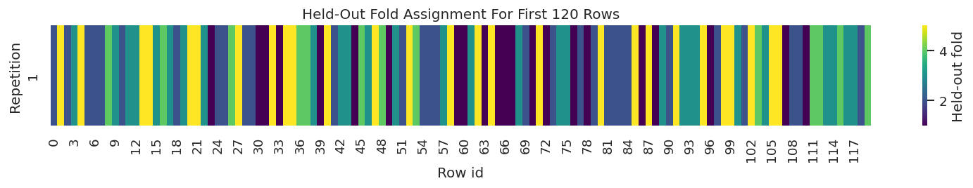
Visualizing Fold Assignments

This cell creates a 5-fold split and displays the fold assignment for the first rows. The heatmap is a compact way to see that every row belongs to exactly one held-out fold in each repetition.

base_splits = make_kfold_splits(plr_df, n_folds=5, seed=RANDOM_SEED)
fold_assignments = fold_assignment_frame([base_splits], n_obs=len(plr_df), n_rep_to_show=1)
fold_preview = fold_assignments.query("row_id < 120").pivot(index="rep", columns="row_id", values="fold")

fold_size_table = (
    fold_assignments.groupby(["rep", "fold"])
    .size()
    .reset_index(name="heldout_rows")
)

save_table(fold_assignments, f"{NOTEBOOK_PREFIX}_fold_assignments.csv")
save_table(fold_size_table, f"{NOTEBOOK_PREFIX}_fold_size_table.csv")

display(fold_size_table)

fig, ax = plt.subplots(figsize=(13, 2.4))
sns.heatmap(fold_preview, cmap="viridis", cbar_kws={"label": "Held-out fold"}, ax=ax)
ax.set_title("Held-Out Fold Assignment For First 120 Rows")
ax.set_xlabel("Row id")
ax.set_ylabel("Repetition")
plt.tight_layout()
fig.savefig(FIGURE_DIR / f"{NOTEBOOK_PREFIX}_fold_assignment_heatmap.png", bbox_inches="tight")
plt.show()

	rep	fold	heldout_rows
0	1	1	192
1	1	2	192
2	1	3	192
3	1	4	192
4	1	5	192

The fold sizes are balanced, and the heatmap shows one held-out fold label per row. DoubleML uses this structure to fit nuisance models and assemble out-of-fold predictions.

Choosing The Number Of Folds

The number of folds controls a trade-off. More folds mean each nuisance model trains on more rows, but there are more nuisance fits. Fewer folds run faster, but each nuisance model trains on less data.

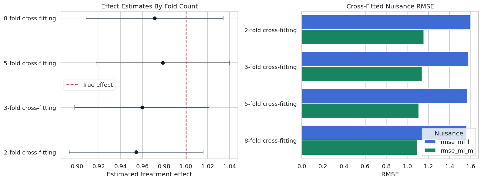
This section compares 2, 3, 5, and 8 folds using the same learner family. The goal is to understand sensitivity, not to find a universally best fold count.

base_learner = HistGradientBoostingRegressor(
    max_iter=80,
    max_leaf_nodes=13,
    min_samples_leaf=20,
    learning_rate=0.06,
    random_state=RANDOM_SEED,
)

fold_rows = []
fold_models = {}
for n_folds in [2, 3, 5, 8]:
    splits = make_kfold_splits(plr_df, n_folds=n_folds, seed=RANDOM_SEED)
    model, row = fit_plr_with_splits(
        plr_df,
        learner=base_learner,
        label=f"{n_folds}-fold cross-fitting",
        n_folds=n_folds,
        n_rep=1,
        all_smpls=splits,
    )
    fold_models[n_folds] = model
    fold_rows.append(row)

fold_comparison = pd.DataFrame(fold_rows)
save_table(fold_comparison, f"{NOTEBOOK_PREFIX}_fold_count_comparison.csv")
display(fold_comparison)

	label	n_folds	n_rep	theta_hat	se	ci_95_lower	ci_95_upper	bias_vs_true	abs_bias_vs_true	rmse_ml_l	rmse_ml_m	mae_ml_l	mae_ml_m	runtime_seconds
0	2-fold cross-fitting	2	1	0.954285	0.031404	0.892734	1.015836	-0.045715	0.045715	1.594533	1.156154	1.265187	0.924849	0.584970
1	3-fold cross-fitting	3	1	0.959661	0.031427	0.898066	1.021257	-0.040339	0.040339	1.580797	1.137801	1.278498	0.909595	0.802480
2	5-fold cross-fitting	5	1	0.978898	0.031306	0.917539	1.040257	-0.021102	0.021102	1.563875	1.108685	1.242786	0.888654	1.295016
3	8-fold cross-fitting	8	1	0.971195	0.032106	0.908268	1.034121	-0.028805	0.028805	1.562304	1.097198	1.244168	0.873190	2.062652

The estimates move modestly across fold counts. That movement is part of split sensitivity. In real work, large swings across reasonable fold counts would be a reason to slow down and inspect nuisance quality, overlap, and sample size.

Fold Count Plot

The next plot shows point estimates, confidence intervals, and nuisance RMSE side by side. This keeps the fold-count choice tied to both causal uncertainty and nuisance prediction quality.

fig, axes = plt.subplots(1, 2, figsize=(13, 5))

axes[0].errorbar(
    x=fold_comparison["theta_hat"],
    y=fold_comparison["label"],
    xerr=1.96 * fold_comparison["se"],
    fmt="o",
    color="#111827",
    ecolor="#475569",
    capsize=4,
)
axes[0].axvline(TRUE_THETA, color="#dc2626", linestyle="--", linewidth=1.5, label="True effect")
axes[0].set_title("Effect Estimates By Fold Count")
axes[0].set_xlabel("Estimated treatment effect")
axes[0].set_ylabel("")
axes[0].legend(loc="best")

rmse_plot = fold_comparison.melt(
    id_vars="label",
    value_vars=["rmse_ml_l", "rmse_ml_m"],
    var_name="nuisance",
    value_name="rmse",
)
sns.barplot(data=rmse_plot, x="rmse", y="label", hue="nuisance", palette=["#2563eb", "#059669"], ax=axes[1])
axes[1].set_title("Cross-Fitted Nuisance RMSE")
axes[1].set_xlabel("RMSE")
axes[1].set_ylabel("")
axes[1].legend(title="Nuisance")

plt.tight_layout()
fig.savefig(FIGURE_DIR / f"{NOTEBOOK_PREFIX}_fold_count_comparison.png", bbox_inches="tight")
plt.show()

The RMSE panel shows that nuisance quality changes with fold count, but not always monotonically. Fold choice is a practical design choice, so reporting it is part of reproducibility.

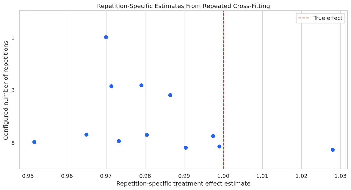
Repeated Cross-Fitting

Repeated cross-fitting draws multiple K-fold partitions and aggregates the resulting estimates. This helps because a single random partition can be lucky or unlucky, especially in smaller samples or when learners are unstable.

DoubleML stores the per-repetition estimates in all_coef and all_se. The aggregate estimate is available as coef and se.

repetition_rows = []
repetition_detail_rows = []
repetition_models = {}

for n_rep in [1, 3, 8]:
    model, row = fit_plr_with_splits(
        plr_df,
        learner=base_learner,
        label=f"5-fold x {n_rep} repetition(s)",
        n_folds=5,
        n_rep=n_rep,
        all_smpls=None,
        seed=RANDOM_SEED,
    )
    repetition_models[n_rep] = model
    repetition_rows.append(row)

    for rep_id, (coef, se) in enumerate(zip(model.all_coef[0], model.all_se[0]), start=1):
        repetition_detail_rows.append(
            {
                "n_rep_setting": n_rep,
                "rep_id": rep_id,
                "theta_hat_rep": float(coef),
                "se_rep": float(se),
                "bias_vs_true": float(coef - TRUE_THETA),
            }
        )

repetition_summary = pd.DataFrame(repetition_rows)
repetition_detail = pd.DataFrame(repetition_detail_rows)

save_table(repetition_summary, f"{NOTEBOOK_PREFIX}_repeated_cross_fitting_summary.csv")
save_table(repetition_detail, f"{NOTEBOOK_PREFIX}_repeated_cross_fitting_detail.csv")

display(repetition_summary)
display(repetition_detail.head(12))

	label	n_folds	n_rep	theta_hat	se	ci_95_lower	ci_95_upper	bias_vs_true	abs_bias_vs_true	rmse_ml_l	rmse_ml_m	mae_ml_l	mae_ml_m	runtime_seconds
0	5-fold x 1 repetition(s)	5	1	0.969909	0.033374	0.904497	1.035320	-0.030091	0.030091	1.550840	1.091125	1.231454	0.871381	1.350095
1	5-fold x 3 repetition(s)	5	3	0.979004	0.032393	0.915515	1.042493	-0.020996	0.020996	1.568709	1.100427	1.253790	0.878583	3.916755
2	5-fold x 8 repetition(s)	5	8	0.985386	0.033241	0.920234	1.050537	-0.014614	0.014614	1.553655	1.106436	1.235832	0.882917	10.016515

	n_rep_setting	rep_id	theta_hat_rep	se_rep	bias_vs_true
0	1	1	0.969909	0.033374	-0.030091
1	3	1	0.986414	0.031716	-0.013586
2	3	2	0.979004	0.032393	-0.020996
3	3	3	0.971292	0.032852	-0.028708
4	8	1	0.964888	0.032001	-0.035112
5	8	2	0.951620	0.033304	-0.048380
6	8	3	0.990378	0.032799	-0.009622
7	8	4	0.998954	0.032592	-0.001046
8	8	5	0.973248	0.032470	-0.026752
9	8	6	1.028002	0.032958	0.028002
10	8	7	0.980393	0.033683	-0.019607
11	8	8	0.997364	0.032066	-0.002636

The detail table shows the estimates from individual repetitions. The aggregate row becomes less dependent on one particular split as the number of repetitions grows.

Repeated Split Distribution

A plot makes repeated cross-fitting easier to understand. Each point below is one repetition-specific estimate; the dashed vertical line is the known true effect.

fig, ax = plt.subplots(figsize=(10, 5.5))
sns.stripplot(
    data=repetition_detail,
    x="theta_hat_rep",
    y="n_rep_setting",
    orient="h",
    size=8,
    jitter=0.16,
    color="#2563eb",
    ax=ax,
)
ax.axvline(TRUE_THETA, color="#dc2626", linestyle="--", linewidth=1.5, label="True effect")
ax.set_title("Repetition-Specific Estimates From Repeated Cross-Fitting")
ax.set_xlabel("Repetition-specific treatment effect estimate")
ax.set_ylabel("Configured number of repetitions")
ax.legend(loc="best")
plt.tight_layout()
fig.savefig(FIGURE_DIR / f"{NOTEBOOK_PREFIX}_repeated_cross_fitting_distribution.png", bbox_inches="tight")
plt.show()

The individual points vary because each repetition uses a different random partition. Repeated cross-fitting is useful when that variation is nontrivial and the extra runtime is acceptable.

External Sample Splits

Sometimes random K-fold splitting is not the right design. If observations are grouped by user, household, region, device, school, or time period, the held-out fold may need to respect that structure.

This section compares ordinary random K-fold splits with GroupKFold splits by user_id. The model controls still exclude user_id; the group is used only to define fold boundaries.

random_group_audit = group_overlap_audit(plr_df, base_splits, group_col="user_id")
group_splits = list(GroupKFold(n_splits=5).split(plr_df, groups=plr_df["user_id"]))
group_split_audit = group_overlap_audit(plr_df, group_splits, group_col="user_id")

random_group_audit["split_type"] = "Random KFold"
group_split_audit["split_type"] = "GroupKFold by user_id"
split_group_audit = pd.concat([random_group_audit, group_split_audit], ignore_index=True)

save_table(split_group_audit, f"{NOTEBOOK_PREFIX}_external_split_group_audit.csv")
display(split_group_audit)

	fold	train_rows	test_rows	train_groups	test_groups	overlap_groups	split_type
0	1	768	192	239	150	149	Random KFold
1	2	768	192	240	143	143	Random KFold
2	3	768	192	238	141	139	Random KFold
3	4	768	192	238	138	136	Random KFold
4	5	768	192	237	133	130	Random KFold
5	1	768	192	192	48	0	GroupKFold by user_id
6	2	768	192	192	48	0	GroupKFold by user_id
7	3	768	192	192	48	0	GroupKFold by user_id
8	4	768	192	192	48	0	GroupKFold by user_id
9	5	768	192	192	48	0	GroupKFold by user_id

Random K-fold splits can place the same user in both training and held-out folds. GroupKFold prevents group overlap, which is often the right validation logic when rows from the same group are closely related.

Random Versus Group-Aware Splits

Now we fit DoubleML with random K-fold splits and with external GroupKFold splits. The comparison shows how to pass a custom split list into DoubleML with set_sample_splitting().

random_split_model, random_split_row = fit_plr_with_splits(
    plr_df,
    learner=base_learner,
    label="External random KFold",
    n_folds=5,
    n_rep=1,
    all_smpls=base_splits,
)

group_split_model, group_split_row = fit_plr_with_splits(
    plr_df,
    learner=base_learner,
    label="External GroupKFold by user_id",
    n_folds=5,
    n_rep=1,
    all_smpls=group_splits,
)

external_split_comparison = pd.DataFrame([random_split_row, group_split_row])
save_table(external_split_comparison, f"{NOTEBOOK_PREFIX}_external_split_comparison.csv")
display(external_split_comparison)

	label	n_folds	n_rep	theta_hat	se	ci_95_lower	ci_95_upper	bias_vs_true	abs_bias_vs_true	rmse_ml_l	rmse_ml_m	mae_ml_l	mae_ml_m	runtime_seconds
0	External random KFold	5	1	0.978898	0.031306	0.917539	1.040257	-0.021102	0.021102	1.563875	1.108685	1.242786	0.888654	1.342976
1	External GroupKFold by user_id	5	1	0.986529	0.031902	0.924002	1.049056	-0.013471	0.013471	1.583457	1.121916	1.258856	0.894433	1.230137

The group-aware estimate is similar in this synthetic data, but the split audit still matters. In real grouped data, preventing group leakage can be more important than a small change in point estimates.

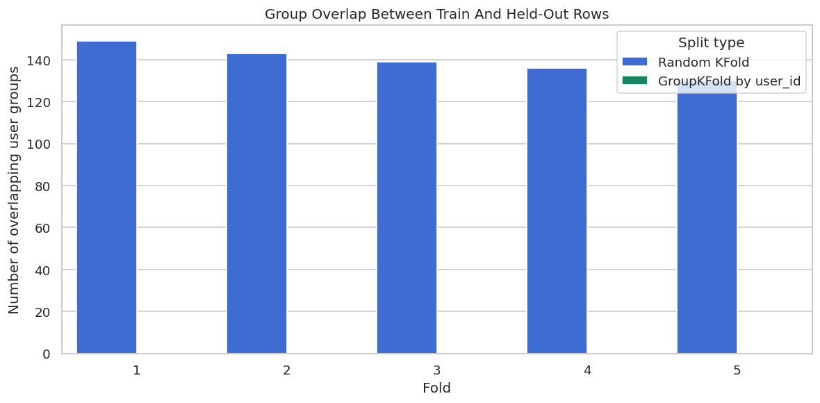
Group Overlap Plot

This plot visualizes the split audit. The goal of GroupKFold is not to change the estimate mechanically; the goal is to enforce a design rule that no user appears in both training and held-out rows for a fold.

fig, ax = plt.subplots(figsize=(10, 5))
sns.barplot(data=split_group_audit, x="fold", y="overlap_groups", hue="split_type", ax=ax, palette=["#2563eb", "#059669"])
ax.set_title("Group Overlap Between Train And Held-Out Rows")
ax.set_xlabel("Fold")
ax.set_ylabel("Number of overlapping user groups")
ax.legend(title="Split type")
plt.tight_layout()
fig.savefig(FIGURE_DIR / f"{NOTEBOOK_PREFIX}_group_overlap_audit.png", bbox_inches="tight")
plt.show()

The GroupKFold bars are zero because each user is held out as a whole unit. That is the central reason to use external splits: they let the analyst encode validation constraints that the default random splitter cannot know.

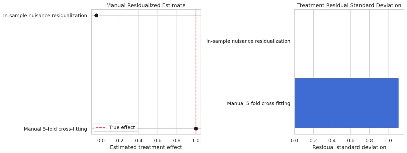
Manual No-Cross-Fitting Caution

DoubleML is designed around out-of-fold nuisance predictions. To see why, we now construct a manual cautionary example with an extremely flexible ExtraTreesRegressor.

The in-sample version fits nuisance models on all rows and predicts those same rows. The cross-fitted version trains on K-1 folds and predicts the held-out fold. Both then run the same residual-on-residual regression.

This is not meant to replace DoubleML’s implementation. It is a visual caution about why in-sample residualization is dangerous.

overfit_learner = ExtraTreesRegressor(
    n_estimators=200,
    min_samples_leaf=1,
    max_features=1.0,
    random_state=RANDOM_SEED,
    n_jobs=1,
)

no_cross_df = plr_df.sample(n=600, random_state=RANDOM_SEED).reset_index(drop=True)
no_cross_x_cols = model_x_cols(no_cross_df)

# In-sample residualization: fit and predict on the same rows.
insample_l = clone(overfit_learner).fit(no_cross_df[no_cross_x_cols], no_cross_df["outcome"])
insample_m = clone(overfit_learner).fit(no_cross_df[no_cross_x_cols], no_cross_df["treatment"])
insample_y_hat = insample_l.predict(no_cross_df[no_cross_x_cols])
insample_d_hat = insample_m.predict(no_cross_df[no_cross_x_cols])
insample_y_res = no_cross_df["outcome"].to_numpy() - insample_y_hat
insample_d_res = no_cross_df["treatment"].to_numpy() - insample_d_hat
insample_theta = LinearRegression(fit_intercept=False).fit(insample_d_res.reshape(-1, 1), insample_y_res).coef_[0]

# Manual cross-fitting: held-out predictions for every row.
cf_y_hat = np.zeros(len(no_cross_df))
cf_d_hat = np.zeros(len(no_cross_df))
manual_splits = make_kfold_splits(no_cross_df, n_folds=5, seed=RANDOM_SEED)
for train_idx, test_idx in manual_splits:
    fold_l = clone(overfit_learner).fit(no_cross_df.iloc[train_idx][no_cross_x_cols], no_cross_df.iloc[train_idx]["outcome"])
    fold_m = clone(overfit_learner).fit(no_cross_df.iloc[train_idx][no_cross_x_cols], no_cross_df.iloc[train_idx]["treatment"])
    cf_y_hat[test_idx] = fold_l.predict(no_cross_df.iloc[test_idx][no_cross_x_cols])
    cf_d_hat[test_idx] = fold_m.predict(no_cross_df.iloc[test_idx][no_cross_x_cols])

cf_y_res = no_cross_df["outcome"].to_numpy() - cf_y_hat
cf_d_res = no_cross_df["treatment"].to_numpy() - cf_d_hat
cf_theta = LinearRegression(fit_intercept=False).fit(cf_d_res.reshape(-1, 1), cf_y_res).coef_[0]

manual_crossfit_comparison = pd.DataFrame(
    [
        {
            "method": "In-sample nuisance residualization",
            "theta_hat": insample_theta,
            "bias_vs_true": insample_theta - TRUE_THETA,
            "outcome_nuisance_rmse": mean_squared_error(no_cross_df["outcome"], insample_y_hat) ** 0.5,
            "treatment_nuisance_rmse": mean_squared_error(no_cross_df["treatment"], insample_d_hat) ** 0.5,
            "treatment_residual_sd": np.std(insample_d_res),
        },
        {
            "method": "Manual 5-fold cross-fitting",
            "theta_hat": cf_theta,
            "bias_vs_true": cf_theta - TRUE_THETA,
            "outcome_nuisance_rmse": mean_squared_error(no_cross_df["outcome"], cf_y_hat) ** 0.5,
            "treatment_nuisance_rmse": mean_squared_error(no_cross_df["treatment"], cf_d_hat) ** 0.5,
            "treatment_residual_sd": np.std(cf_d_res),
        },
    ]
)

save_table(manual_crossfit_comparison, f"{NOTEBOOK_PREFIX}_manual_no_cross_fit_caution.csv")
display(manual_crossfit_comparison)

	method	theta_hat	bias_vs_true	outcome_nuisance_rmse	treatment_nuisance_rmse	treatment_residual_sd
0	In-sample nuisance residualization	-0.049285	-1.049285	5.766047e-15	3.803450e-15	3.802177e-15
1	Manual 5-fold cross-fitting	1.000418	0.000418	1.627348e+00	1.114617e+00	1.114522e+00

The in-sample nuisance RMSE is almost zero because the flexible trees can interpolate the training rows. That looks excellent as prediction output, but it destroys the residual structure needed for causal estimation. The cross-fitted residuals are noisier in a healthy way: they are honest held-out residuals.

No-Cross-Fitting Caution Plot

The plot below puts the cautionary comparison on two panels: effect estimate and treatment-residual standard deviation. The in-sample residual standard deviation can become tiny when the learner memorizes the training data.

fig, axes = plt.subplots(1, 2, figsize=(13, 5))

sns.scatterplot(
    data=manual_crossfit_comparison,
    x="theta_hat",
    y="method",
    s=90,
    color="#111827",
    ax=axes[0],
)
axes[0].axvline(TRUE_THETA, color="#dc2626", linestyle="--", linewidth=1.5, label="True effect")
axes[0].set_title("Manual Residualized Estimate")
axes[0].set_xlabel("Estimated treatment effect")
axes[0].set_ylabel("")
axes[0].legend(loc="best")

sns.barplot(data=manual_crossfit_comparison, x="treatment_residual_sd", y="method", color="#2563eb", ax=axes[1])
axes[1].set_title("Treatment Residual Standard Deviation")
axes[1].set_xlabel("Residual standard deviation")
axes[1].set_ylabel("")

plt.tight_layout()
fig.savefig(FIGURE_DIR / f"{NOTEBOOK_PREFIX}_manual_no_cross_fit_caution.png", bbox_inches="tight")
plt.show()

This is the clearest practical reason for cross-fitting: training-set predictions can be too good to be useful. The causal score needs held-out nuisance predictions, not memorized training residuals.

Split Reporting Checklist

A reproducible DoubleML analysis should document its split design. This checklist can be copied into applied notebooks and reports.

split_reporting_checklist = pd.DataFrame(
    [
        {"item": "State number of folds", "why": "Fold count changes training size and number of nuisance fits."},
        {"item": "State number of repetitions", "why": "Repeated cross-fitting affects split stability and runtime."},
        {"item": "Record random seeds", "why": "Random sample splits should be reproducible."},
        {"item": "Explain external split constraints", "why": "Grouped, clustered, or temporal data often require custom split logic."},
        {"item": "Report nuisance prediction diagnostics", "why": "Split design should be assessed with held-out nuisance performance."},
        {"item": "Show split sensitivity when material", "why": "Large changes across reasonable splits weaken confidence in one estimate."},
        {"item": "Avoid in-sample nuisance residualization", "why": "Flexible learners can memorize rows and distort the orthogonal score."},
    ]
)

save_table(split_reporting_checklist, f"{NOTEBOOK_PREFIX}_split_reporting_checklist.csv")
display(split_reporting_checklist)

	item	why
0	State number of folds	Fold count changes training size and number of...
1	State number of repetitions	Repeated cross-fitting affects split stability...
2	Record random seeds	Random sample splits should be reproducible.
3	Explain external split constraints	Grouped, clustered, or temporal data often req...
4	Report nuisance prediction diagnostics	Split design should be assessed with held-out ...
5	Show split sensitivity when material	Large changes across reasonable splits weaken ...
6	Avoid in-sample nuisance residualization	Flexible learners can memorize rows and distor...

The checklist makes split design part of the causal audit trail. It also helps separate honest split sensitivity from casual rerunning until a pleasing estimate appears.

Report Template And Artifact Manifest

The final cell writes a short split-design report template and an artifact manifest. The template is intentionally concise, but it includes the details that should be visible in a serious DoubleML write-up.

report_text = f"""
# Sample Splitting And Cross-Fitting Report Template

## Model
- DoubleML model class:
- Treatment:
- Outcome:
- Control set:
- Primary learner:

## Split Design
- Number of folds:
- Number of repetitions:
- Random seed(s):
- Internal or external splits:
- Group, cluster, or time constraints:

## Diagnostics
- Outcome nuisance RMSE:
- Treatment nuisance RMSE:
- Split sensitivity across fold counts:
- Repetition-specific estimate range:
- Group overlap audit, if applicable:

## Final Estimate
- Point estimate:
- Standard error:
- Confidence interval:
- Split-related caveats:
""".strip()

report_path = REPORT_DIR / f"{NOTEBOOK_PREFIX}_sample_splitting_report_template.md"
report_path.write_text(report_text)

artifact_manifest = pd.DataFrame(
    [
        {"artifact": "synthetic PLR data", "path": str(DATASET_DIR / f"{NOTEBOOK_PREFIX}_synthetic_panel_like_plr_data.csv")},
        {"artifact": "fold count comparison", "path": str(TABLE_DIR / f"{NOTEBOOK_PREFIX}_fold_count_comparison.csv")},
        {"artifact": "repeated cross-fitting summary", "path": str(TABLE_DIR / f"{NOTEBOOK_PREFIX}_repeated_cross_fitting_summary.csv")},
        {"artifact": "external split audit", "path": str(TABLE_DIR / f"{NOTEBOOK_PREFIX}_external_split_group_audit.csv")},
        {"artifact": "manual no-cross-fit caution", "path": str(TABLE_DIR / f"{NOTEBOOK_PREFIX}_manual_no_cross_fit_caution.csv")},
        {"artifact": "report template", "path": str(report_path)},
        {"artifact": "cross-fitting workflow figure", "path": str(FIGURE_DIR / f"{NOTEBOOK_PREFIX}_cross_fitting_workflow.png")},
        {"artifact": "fold assignment heatmap", "path": str(FIGURE_DIR / f"{NOTEBOOK_PREFIX}_fold_assignment_heatmap.png")},
    ]
)

save_table(artifact_manifest, f"{NOTEBOOK_PREFIX}_artifact_manifest.csv")
display(Markdown(f"Report template written to `{report_path}`"))
display(artifact_manifest)

Report template written to /home/apex/Documents/ranking_sys/notebooks/tutorials/doubleml/outputs/reports/11_sample_splitting_report_template.md

	artifact	path
0	synthetic PLR data	/home/apex/Documents/ranking_sys/notebooks/tut...
1	fold count comparison	/home/apex/Documents/ranking_sys/notebooks/tut...
2	repeated cross-fitting summary	/home/apex/Documents/ranking_sys/notebooks/tut...
3	external split audit	/home/apex/Documents/ranking_sys/notebooks/tut...
4	manual no-cross-fit caution	/home/apex/Documents/ranking_sys/notebooks/tut...
5	report template	/home/apex/Documents/ranking_sys/notebooks/tut...
6	cross-fitting workflow figure	/home/apex/Documents/ranking_sys/notebooks/tut...
7	fold assignment heatmap	/home/apex/Documents/ranking_sys/notebooks/tut...

The notebook now has a full split-design workflow: theory, API mechanics, fold-count sensitivity, repeated cross-fitting, external group splits, and a concrete warning against in-sample residualization.

What Comes Next

The next natural topic is inference: standard errors, confidence intervals, bootstrap options, joint inference, and how to communicate uncertainty from DoubleML estimates.