This notebook teaches regression discontinuity design with DoubleML and the RDD tools available in the installed environment.
RDD is a local causal design. Treatment changes sharply or probabilistically at a cutoff in a running variable. The causal claim is not that treated and untreated units are comparable everywhere. The claim is narrower: units just below and just above the cutoff are comparable except for treatment assignment.
That local nature makes RDD both powerful and limited. It can be credible when the cutoff rule is real and hard to manipulate, but the estimand is usually a cutoff-local effect. A good RDD notebook therefore needs more than a single coefficient: it needs a running-variable plot, cutoff support checks, covariate continuity checks, bandwidth sensitivity, and clear reporting of the local target.
Learning Goals
By the end of this notebook, you should be able to:
define the sharp and fuzzy RDD estimands;
explain the continuity assumption at the cutoff;
distinguish global treatment comparisons from local cutoff comparisons;
construct DoubleMLRDDData with outcome, treatment, running score, and covariates;
fit conventional rdrobust estimates and flexible RDFlex estimates;
audit running-variable support, density, and covariate continuity;
compare estimates across bandwidths;
report RDD results with assumptions and local-scope caveats.
RDD Intuition
An RDD starts with a score or running variable. Examples include an eligibility score, age, income, risk score, rating threshold, time relative to a cutoff, or an assignment priority index.
The cutoff creates a rule:
D = 1 if score >= cutoff
D = 0 if score < cutoff
In a sharp RDD, the rule determines treatment exactly. In a fuzzy RDD, crossing the cutoff changes the probability of treatment, but some units do not comply with the cutoff rule.
The RDD estimand is a limit comparison:
lim E[Y | score = cutoff from the right]
-
lim E[Y | score = cutoff from the left]
For fuzzy RDD, that outcome jump is divided by the treatment jump. This gives a local treatment effect for units whose treatment status is shifted by crossing the cutoff.
Identification Assumptions
RDD identification relies on continuity near the cutoff. Potential outcomes should evolve smoothly through the cutoff in the absence of treatment. If units cannot precisely manipulate which side of the cutoff they land on, observations just below and just above the cutoff can be treated as locally comparable.
Important assumptions and diagnostics:
Continuity of potential outcomes: without treatment, the conditional mean outcome would be smooth at the cutoff.
No precise manipulation: units should not sort around the cutoff in a way that creates a discontinuity in unobserved determinants of the outcome.
Covariate continuity: pre-treatment covariates should not jump at the cutoff.
Local support: there should be enough observations on both sides near the cutoff.
Bandwidth sensitivity: estimates should not depend entirely on one arbitrary window around the cutoff.
These diagnostics support the design story. They do not prove the assumption, but they make the argument more transparent.
Where DoubleML Fits
Classic RDD uses local polynomial regression around the cutoff. rdrobust is a common implementation for bandwidth selection, bias correction, and robust intervals.
DoubleML adds a flexible adjustment workflow through DoubleMLRDDData and RDFlex. The idea is to use machine learning to adjust for observed covariates while preserving the local RDD logic. The running variable and cutoff still drive identification; machine learning is not a substitute for the cutoff design.
The installed environment has:
DoubleMLRDDData for the RDD data backend;
doubleml.rdd.RDFlex for flexible RDD adjustment;
rdrobust for conventional RDD estimates.
Runtime Note
This notebook fits conventional RDD estimates, flexible sharp RDD estimates, and a fuzzy RDD example. A full run should take about 1 to 3 minutes on a typical laptop.
Setup
The setup cell imports the scientific Python stack, DoubleML RDD classes, and rdrobust. A narrow warning filter suppresses an import-time rdrobustSyntaxWarning that is unrelated to this tutorial’s computations.
The package table confirms that the optional RDD pieces are available in this environment. If this notebook is moved to another machine and the RDD imports fail, install the optional dependency with uv add "doubleml[rdd]".
Helper Functions
The helper functions below implement transparent RDD calculations and output formatting. The manual local-linear estimates are not a replacement for rdrobust; they are included so the mechanics of bandwidth windows, side-specific slopes, and triangular weights are easy to see.
def save_table(df, file_name, index=False):"""Save a table under the notebook output folder and return the DataFrame.""" path = TABLE_DIR / file_name df.to_csv(path, index=index)return dfdef triangular_kernel(centered_score, bandwidth):"""Triangular kernel weights for observations inside a bandwidth.""" distance = np.abs(centered_score) / bandwidthreturn np.clip(1.0- distance, 0.0, None)def local_linear_rdd(df, y_col, score_col, cutoff=0.0, bandwidth=0.30, covariates=None, fuzzy_d_col=None):"""Estimate a local-linear sharp or fuzzy RDD with triangular weights.""" covariates = covariates or [] work = df.loc[np.abs(df[score_col] - cutoff) <= bandwidth].copy() work["centered_score"] = work[score_col] - cutoff work["right_of_cutoff"] = (work["centered_score"] >=0).astype(int) work["score_x_right"] = work["centered_score"] * work["right_of_cutoff"] weights = triangular_kernel(work["centered_score"].to_numpy(), bandwidth) x_cols = ["right_of_cutoff", "centered_score", "score_x_right"] + covariates X = sm.add_constant(work[x_cols], has_constant="add") y = work[y_col] reduced_form = sm.WLS(y, X, weights=weights).fit(cov_type="HC1") reduced_jump =float(reduced_form.params["right_of_cutoff"]) reduced_se =float(reduced_form.bse["right_of_cutoff"])if fuzzy_d_col isNone:return {"bandwidth": bandwidth,"n_window": len(work),"n_left": int((work["centered_score"] <0).sum()),"n_right": int((work["centered_score"] >=0).sum()),"estimate": reduced_jump,"std_error": reduced_se,"ci_95_lower": reduced_jump -1.96* reduced_se,"ci_95_upper": reduced_jump +1.96* reduced_se,"reduced_form_jump": reduced_jump,"first_stage_jump": np.nan, } first_stage = sm.WLS(work[fuzzy_d_col], X, weights=weights).fit(cov_type="HC1") first_jump =float(first_stage.params["right_of_cutoff"]) first_se =float(first_stage.bse["right_of_cutoff"]) fuzzy_estimate = reduced_jump / first_jump# A simple delta-method approximation that ignores covariance between first stage and reduced form. fuzzy_se =abs(fuzzy_estimate) * np.sqrt((reduced_se / reduced_jump) **2+ (first_se / first_jump) **2)return {"bandwidth": bandwidth,"n_window": len(work),"n_left": int((work["centered_score"] <0).sum()),"n_right": int((work["centered_score"] >=0).sum()),"estimate": fuzzy_estimate,"std_error": fuzzy_se,"ci_95_lower": fuzzy_estimate -1.96* fuzzy_se,"ci_95_upper": fuzzy_estimate +1.96* fuzzy_se,"reduced_form_jump": reduced_jump,"first_stage_jump": first_jump, }def rdrobust_summary(result, label, design, true_target):"""Extract conventional, bias-corrected, and robust rows from an rdrobust result.""" rows = []for method in result.coef.index: coef =float(result.coef.loc[method].iloc[0]) ci_low =float(result.ci.loc[method].iloc[0]) ci_high =float(result.ci.loc[method].iloc[1]) rows.append( {"estimator": f"{label} - {method}","design": design,"theta_hat": coef,"ci_95_lower": ci_low,"ci_95_upper": ci_high,"true_target": true_target,"bias_vs_target": coef - true_target, } )return pd.DataFrame(rows)def rdflex_summary(model, label, design, true_target):"""Extract conventional, bias-corrected, and robust rows from a fitted RDFlex object.""" method_names = ["Conventional", "Bias-Corrected", "Robust"] ci = model.confint(level=0.95) rows = []for i, method inenumerate(method_names): theta =float(model.coef[i]) se =float(model.se[i]) rows.append( {"estimator": f"{label} - {method}","design": design,"theta_hat": theta,"std_error": se,"ci_95_lower": float(ci.iloc[i, 0]),"ci_95_upper": float(ci.iloc[i, 1]),"true_target": true_target,"bias_vs_target": theta - true_target, } )return pd.DataFrame(rows)def add_ci_columns(df):"""Prepare lower and upper error-bar columns for plotting.""" out = df.copy() out["lower_error"] = out["theta_hat"] - out["ci_95_lower"] out["upper_error"] = out["ci_95_upper"] - out["theta_hat"]return out
The local-linear helper uses the standard RDD idea: fit separate local slopes on the left and right of the cutoff and read the discontinuity as the treatment effect. The flexible DoubleML estimator will later use machine-learning adjustment before applying RDD estimation logic.
Teaching Diagram
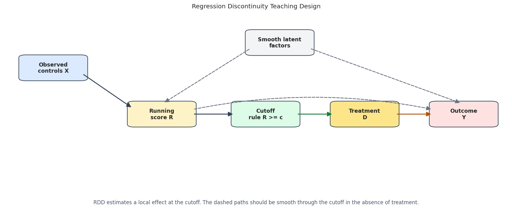
The RDD diagram is simpler than many causal diagrams because the key object is the cutoff. The running variable determines treatment status near the cutoff, and the outcome can vary smoothly with the running variable even without treatment.
from matplotlib.patches import FancyArrowPatch, FancyBboxPatch# The nodes are intentionally spaced across a wider canvas so the direction of the# assignment path is easy to read. Smaller boxes also leave longer visible arrow lines.nodes = {"X": {"xy": (0.07, 0.74), "label": "Observed\ncontrols X", "color": "#dbeafe"},"R": {"xy": (0.30, 0.52), "label": "Running\nscore R", "color": "#fef3c7"},"C": {"xy": (0.52, 0.52), "label": "Cutoff\nrule R >= c", "color": "#dcfce7"},"D": {"xy": (0.73, 0.52), "label": "Treatment\nD", "color": "#fde68a"},"Y": {"xy": (0.94, 0.52), "label": "Outcome\nY", "color": "#fee2e2"},"U": {"xy": (0.55, 0.86), "label": "Smooth latent\nfactors", "color": "#f3f4f6"},}fig, ax = plt.subplots(figsize=(14, 6.2))ax.set_axis_off()ax.set_xlim(-0.035, 1.035)ax.set_ylim(0.02, 0.98)box_w, box_h =0.118, 0.095arrow_gap =0.010def anchor(node, side): x, y = nodes[node]["xy"] offsets = {"left": (-box_w /2, 0),"right": (box_w /2, 0),"top": (0, box_h /2),"bottom": (0, -box_h /2),"upper_right": (box_w /2, box_h *0.25),"lower_right": (box_w /2, -box_h *0.25),"upper_left": (-box_w /2, box_h *0.25),"lower_left": (-box_w /2, -box_h *0.25), } dx, dy = offsets[side]return np.array([x + dx, y + dy], dtype=float)def shorten(start, end, gap=arrow_gap): start = np.asarray(start, dtype=float) end = np.asarray(end, dtype=float) delta = end - start length = np.hypot(delta[0], delta[1])if length ==0:returntuple(start), tuple(end) unit = delta / lengthreturntuple(start + gap * unit), tuple(end - gap * unit)def draw_arrow(start, end, color, style="solid", rad=0.0, linewidth=1.7): start, end = shorten(start, end) arrow = FancyArrowPatch( start, end, arrowstyle="-|>", mutation_scale=18, linewidth=linewidth, color=color, linestyle=style, shrinkA=0, shrinkB=0, connectionstyle=f"arc3,rad={rad}", zorder=5, ) ax.add_patch(arrow)# Main assignment path.draw_arrow(anchor("X", "lower_right"), anchor("R", "upper_left"), color="#334155")draw_arrow(anchor("R", "right"), anchor("C", "left"), color="#334155")draw_arrow(anchor("C", "right"), anchor("D", "left"), color="#15803d")draw_arrow(anchor("D", "right"), anchor("Y", "left"), color="#b45309")# Smooth background paths remind us what continuity means.draw_arrow(anchor("R", "upper_right"), anchor("Y", "upper_left"), color="#6b7280", style="dashed", rad=-0.10, linewidth=1.5)draw_arrow(anchor("U", "lower_left"), anchor("R", "top"), color="#6b7280", style="dashed", linewidth=1.5)draw_arrow(anchor("U", "lower_right"), anchor("Y", "top"), color="#6b7280", style="dashed", linewidth=1.5)for spec in nodes.values(): x, y = spec["xy"] rect = FancyBboxPatch( (x - box_w /2, y - box_h /2), box_w, box_h, boxstyle="round,pad=0.014", facecolor=spec["color"], edgecolor="#334155", linewidth=1.2, zorder=3, ) ax.add_patch(rect) ax.text(x, y, spec["label"], ha="center", va="center", fontsize=10.5, fontweight="bold", zorder=4)ax.text(0.50,0.10,"RDD estimates a local effect at the cutoff. The dashed paths should be smooth through the cutoff in the absence of treatment.", ha="center", va="center", fontsize=10, color="#475569",)ax.set_title("Regression Discontinuity Teaching Design", pad=18)plt.tight_layout()fig.savefig(FIGURE_DIR /f"{NOTEBOOK_PREFIX}_rdd_design_dag.png", dpi=160, bbox_inches="tight")plt.show()
The diagram highlights the central design logic. The running score can affect the outcome smoothly, but the discontinuous change in treatment at the cutoff is what identifies the local effect.
Synthetic Sharp RDD Data
The first dataset is a sharp RDD. Treatment is exactly assigned by whether the running score is above the cutoff. The outcome also depends smoothly on the score and observed covariates. The true jump at the cutoff is 1.2.
Because this is synthetic data, we know the truth. In real data, the best we can do is argue that the cutoff is credible and show diagnostics.
Rows: 4,500
Cutoff: 0.0
True sharp RDD effect at cutoff: 1.200
Saved data to: notebooks/tutorials/doubleml/outputs/datasets/09_synthetic_sharp_rdd.csv
row_id
outcome
treatment
running_score
engagement_score
baseline_value
mobile_user
smooth_score_component
true_effect_at_cutoff
0
0
4.935937
1
0.547912
0.065983
0.890045
0
0.949672
1.2
1
1
0.528297
0
-0.122243
-0.464412
1.299978
0
-0.158546
1.2
2
2
3.570701
1
0.717196
-1.014069
-0.110422
0
1.286454
1.2
3
3
3.740875
1
0.394736
-1.266596
-0.862670
1
0.655756
1.2
4
4
1.158950
0
-0.811645
-0.048484
2.109985
1
-0.422149
1.2
Treatment switches exactly at the cutoff. The outcome is not flat in the running score, which is realistic. RDD does not require the outcome to be flat; it requires the no-treatment outcome function to be smooth through the cutoff.
Sharp RDD Field Dictionary
The field dictionary makes the causal roles explicit. The running score is not an ordinary control; it is the assignment variable that defines the local comparison.
The most important roles are running_score, treatment, and outcome. If the cutoff rule is incorrectly encoded, every downstream estimate answers the wrong question.
Basic Audit And Local Support
The first audit checks sample size, treatment share, and how many observations fall near the cutoff. RDD is a local design, so the rows near zero matter most.
The local windows have observations on both sides of the cutoff. That is a minimal requirement for RDD; without local support, the estimate would be extrapolation rather than a local comparison.
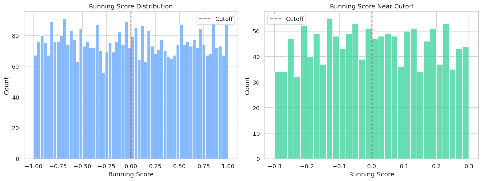
Running-Variable Distribution
A running-variable density check looks for suspicious bunching around the cutoff. In real data, a large density jump can suggest manipulation or sorting. Here the score is generated smoothly, so no jump should appear.
The histogram is smooth around the cutoff. That supports the no-precise-manipulation story in this synthetic setting.
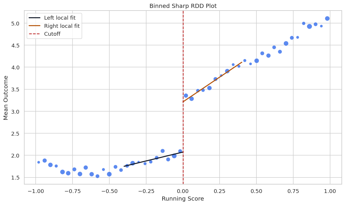
Binned RDD Plot
The binned plot is the classic first RDD visualization. It shows average outcomes in running-score bins and overlays local linear fits near the cutoff.
The jump at the cutoff is visible, while the outcome also changes smoothly with the running score. That is exactly the pattern RDD is designed to handle.
Covariate Continuity Checks
Pre-assignment covariates should not jump at the cutoff. If they do, observations just above and below the cutoff may not be locally comparable.
The table below estimates local discontinuities in each covariate using the same local-linear helper.
The covariate jumps are small relative to their uncertainty. That is what we expect in the synthetic design because covariates were generated smoothly with respect to the score.
Manual Local-Linear RDD Estimates
Now we estimate the sharp RDD effect manually across bandwidths. Narrow bandwidths are more local but noisier. Wider bandwidths are more precise but rely more heavily on functional-form approximation away from the cutoff.
The estimates are reasonably stable across bandwidths. Covariate adjustment can improve precision, but the running-score cutoff still supplies the identifying variation.
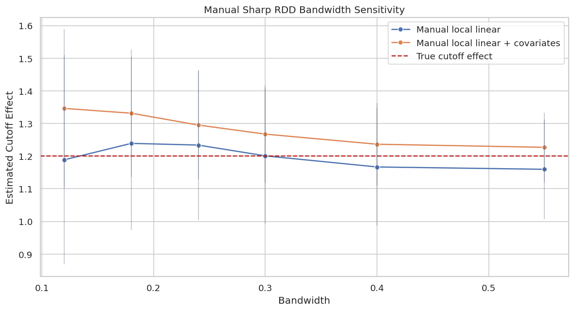
Bandwidth Sensitivity Plot
A plot makes bandwidth sensitivity easier to inspect than a table. We want estimates to move somewhat as bandwidth changes, but not to tell completely different stories across reasonable windows.
The plot shows the bias-variance tradeoff. The smallest windows are noisier, while very wide windows can be more sensitive to curvature away from the cutoff.
Conventional rdrobust Estimate
rdrobust is a standard RDD tool for local-polynomial estimation, bandwidth selection, bias correction, and robust confidence intervals. The output reports conventional, bias-corrected, and robust rows.
Call: rdrobust
Number of Observations:                  4500
Polynomial Order Est. (p):                  1
Polynomial Order Bias (q):                  2
Kernel:                            Triangular
Bandwidth Selection:                    mserd
Var-Cov Estimator:                         NN

                                Left      Right
------------------------------------------------
Number of Observations          2270       2230
Number of Unique Obs.           2270       2230
Number of Effective Obs.         582        579
Bandwidth Estimation           0.254      0.254
Bandwidth Bias                 0.399      0.399
rho (h/b)                      0.636      0.636

Method             Coef.     S.E.   t-stat    P>|t|       95% CI
-------------------------------------------------------------------------
Conventional       1.227    0.116   10.574   3.929e-26     [0.999, 1.454]
Robust                 -        -    9.169   4.785e-20     [0.988, 1.526]
estimator
design
theta_hat
ci_95_lower
ci_95_upper
true_target
bias_vs_target
0
rdrobust sharp - Conventional
sharp RDD
1.226608
0.999250
1.453966
1.2
0.026608
1
rdrobust sharp - Bias-Corrected
sharp RDD
1.257036
1.029678
1.484394
1.2
0.057036
2
rdrobust sharp - Robust
sharp RDD
1.257036
0.988325
1.525747
1.2
0.057036
The robust interval is usually the row to emphasize from rdrobust, while the conventional row is useful for orientation. The estimate is close to the true cutoff jump in this synthetic design.
DoubleML RDD Data Backend
DoubleMLRDDData gives DoubleML the outcome, treatment, running score, and optional covariates. The score column has a special role; it is not simply another predictor.
This backend object is the contract for the flexible RDD estimator. If score_col is wrong, the cutoff comparison is wrong.
Fit RDFlex For Sharp RDD
RDFlex uses machine-learning adjustment for covariates and then applies RDD estimation logic. The learner for ml_g must support sample_weight; the tree learners used here do.
The flexible estimates are close to the cutoff effect. Differences across learners are expected because the nuisance adjustment is learned from data and the estimate remains local.
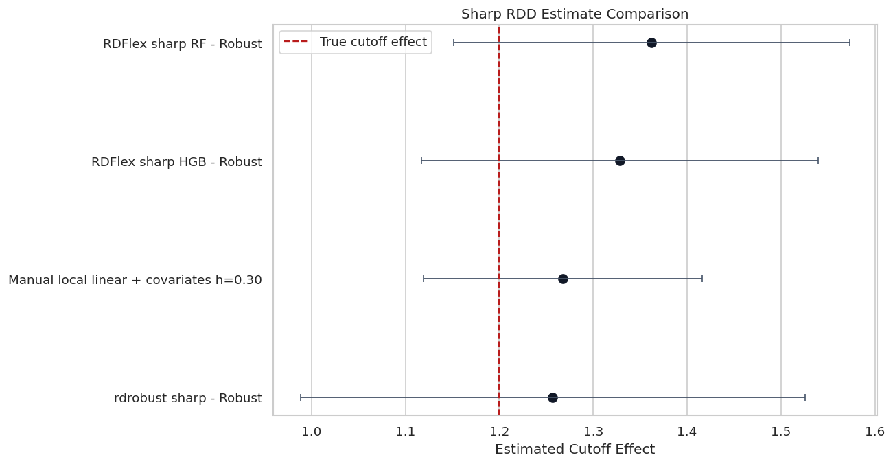
Sharp RDD Estimate Comparison
This plot combines manual local-linear estimates, rdrobust, and RDFlex. It focuses on the robust or main rows rather than showing every row from every estimator.
The estimates tell the same broad story: there is a positive jump at the cutoff close to the true value. The interval widths remind us that RDD uses only local information, so precision depends heavily on near-cutoff sample size.
Synthetic Fuzzy RDD Data
In a fuzzy RDD, crossing the cutoff changes treatment probability but does not perfectly determine treatment. The cutoff becomes an instrument for treatment.
The target is a local treatment effect for units whose treatment status is shifted by crossing the cutoff. In this synthetic example, the true treatment effect is constant at 1.0, so the fuzzy local effect is also 1.0.
Rows: 5,000
True fuzzy local effect: 1.000
Treatment jump near cutoff, h=0.05: 0.512
Saved data to: notebooks/tutorials/doubleml/outputs/datasets/09_synthetic_fuzzy_rdd.csv
row_id
outcome
treatment
running_score
cutoff_offer
engagement_score
baseline_value
mobile_user
true_treatment_probability
true_effect_at_cutoff
0
0
2.436736
0
-0.173360
0
0.532258
0.219500
0
0.223964
1.0
1
1
4.890023
1
0.953584
1
-0.635429
-0.054437
1
0.786693
1.0
2
2
2.495195
0
0.011308
1
-0.704889
0.184743
0
0.698270
1.0
3
3
1.805403
0
0.308595
1
-1.094973
1.137687
0
0.664431
1.0
4
4
2.453631
0
0.415557
1
-0.486513
-0.562355
1
0.771413
1.0
The cutoff creates a large jump in treatment probability, but treatment is not deterministic. That is the fuzzy RDD setting.
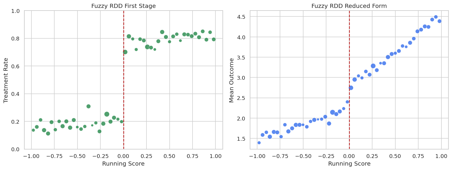
Fuzzy First Stage Plot
The first-stage plot checks whether the cutoff actually changes treatment probability. Without a visible first stage, a fuzzy RDD has little identifying variation.
The treatment rate jumps at the cutoff. The outcome also jumps, but the fuzzy treatment effect is the outcome jump divided by the treatment jump.
Fuzzy RDD Estimates
We estimate the fuzzy RDD with both rdrobust and RDFlex. RDFlex receives an outcome learner and a treatment learner because treatment is no longer deterministic at the cutoff.
Call: rdrobust
Number of Observations:                  5000
Polynomial Order Est. (p):                  1
Polynomial Order Bias (q):                  2
Kernel:                            Triangular
Bandwidth Selection:                    mserd
Var-Cov Estimator:                         NN

                                Left      Right
------------------------------------------------
Number of Observations          2493       2507
Number of Unique Obs.           2493       2507
Number of Effective Obs.        1021       1037
Bandwidth Estimation           0.408      0.408
Bandwidth Bias                 0.617      0.617
rho (h/b)                      0.661      0.661

Method             Coef.     S.E.   t-stat    P>|t|       95% CI
-------------------------------------------------------------------------
Conventional       0.835    0.153    5.446   5.154e-08     [0.534, 1.135]
Robust                 -        -    4.069   4.720e-05     [0.388, 1.109]
estimator
design
theta_hat
ci_95_lower
ci_95_upper
true_target
bias_vs_target
0
rdrobust fuzzy - Conventional
fuzzy RDD
0.834834
0.534380
1.135288
1.0
-0.165166
1
rdrobust fuzzy - Bias-Corrected
fuzzy RDD
0.748283
0.447829
1.048737
1.0
-0.251717
2
rdrobust fuzzy - Robust
fuzzy RDD
0.748283
0.387857
1.108709
1.0
-0.251717
bandwidth
n_window
n_left
n_right
estimate
std_error
ci_95_lower
ci_95_upper
reduced_form_jump
first_stage_jump
estimator
true_target
bias_vs_target
0
0.18
908
455
453
0.984543
0.230390
0.532979
1.436106
0.514370
0.522446
Manual fuzzy local linear + covariates
1.0
-0.015457
1
0.24
1233
627
606
0.989449
0.194074
0.609063
1.369834
0.535428
0.541138
Manual fuzzy local linear + covariates
1.0
-0.010551
2
0.30
1555
772
783
1.009756
0.175413
0.665946
1.353565
0.547735
0.542443
Manual fuzzy local linear + covariates
1.0
0.009756
3
0.40
2017
1002
1015
1.022569
0.153939
0.720849
1.324290
0.559048
0.546709
Manual fuzzy local linear + covariates
1.0
0.022569
estimator
design
theta_hat
std_error
ci_95_lower
ci_95_upper
true_target
bias_vs_target
0
RDFlex fuzzy HGB - Conventional
fuzzy RDD
0.999605
0.124314
0.755955
1.243256
1.0
-0.000395
1
RDFlex fuzzy HGB - Bias-Corrected
fuzzy RDD
0.980319
0.124314
0.736668
1.223969
1.0
-0.019681
2
RDFlex fuzzy HGB - Robust
fuzzy RDD
0.980319
0.145337
0.695464
1.265174
1.0
-0.019681
The fuzzy estimates are close to the true local treatment effect. They are less precise than the sharp estimates because the cutoff only partially shifts treatment.
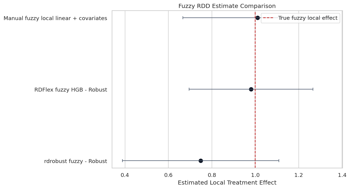
Fuzzy Estimate Comparison
The fuzzy comparison plot shows the robust rdrobust estimate, the RDFlex robust estimate, and a manual local-linear estimate at a representative bandwidth.
The fuzzy estimates agree on a positive local treatment effect. The wider intervals reflect the extra uncertainty from estimating the first-stage treatment jump.
Reporting Checklist
RDD reporting should focus on the cutoff design. A polished RDD report should name the running variable, cutoff, bandwidth, local target, and diagnostics.
rdd_reporting_checklist = pd.DataFrame( [ {"topic": "running variable", "question": "What score determines treatment eligibility?", "notebook_answer": "running_score."}, {"topic": "cutoff", "question": "Where does assignment change?", "notebook_answer": f"Cutoff is {CUTOFF}."}, {"topic": "design type", "question": "Is treatment sharp or fuzzy at the cutoff?", "notebook_answer": "Both sharp and fuzzy examples are demonstrated."}, {"topic": "estimand", "question": "Is the effect local or global?", "notebook_answer": "Local effect at the cutoff."}, {"topic": "support", "question": "Are there enough observations on both sides near the cutoff?", "notebook_answer": "Checked through local window counts."}, {"topic": "manipulation", "question": "Is there suspicious bunching at the cutoff?", "notebook_answer": "Checked through running-score histograms."}, {"topic": "covariate continuity", "question": "Do pre-treatment covariates jump at the cutoff?", "notebook_answer": "Checked with local-linear covariate discontinuities."}, {"topic": "bandwidth", "question": "Does the estimate change across reasonable bandwidths?", "notebook_answer": "Checked through bandwidth sensitivity."}, {"topic": "fuzzy first stage", "question": "Does cutoff crossing shift treatment probability?", "notebook_answer": "Checked in the fuzzy first-stage plot."}, ])save_table(rdd_reporting_checklist, f"{NOTEBOOK_PREFIX}_rdd_reporting_checklist.csv")display(rdd_reporting_checklist)
topic
question
notebook_answer
0
running variable
What score determines treatment eligibility?
running_score.
1
cutoff
Where does assignment change?
Cutoff is 0.0.
2
design type
Is treatment sharp or fuzzy at the cutoff?
Both sharp and fuzzy examples are demonstrated.
3
estimand
Is the effect local or global?
Local effect at the cutoff.
4
support
Are there enough observations on both sides ne...
Checked through local window counts.
5
manipulation
Is there suspicious bunching at the cutoff?
Checked through running-score histograms.
6
covariate continuity
Do pre-treatment covariates jump at the cutoff?
Checked with local-linear covariate discontinu...
7
bandwidth
Does the estimate change across reasonable ban...
Checked through bandwidth sensitivity.
8
fuzzy first stage
Does cutoff crossing shift treatment probability?
Checked in the fuzzy first-stage plot.
This checklist keeps the RDD estimate connected to its design. The strongest RDD reports are usually visual and diagnostic, not just model-summary tables.
Report Template
The report template below writes a concise RDD summary using the preferred robust rows. It also states the local nature of the effect.
best_sharp = sharp_estimate_comparison.loc[sharp_estimate_comparison["estimator"] =="RDFlex sharp HGB - Robust"].iloc[0]best_fuzzy = fuzzy_estimate_comparison.loc[fuzzy_estimate_comparison["estimator"] =="RDFlex fuzzy HGB - Robust"].iloc[0]report_text =f"""# Regression Discontinuity DoubleML Report Template## QuestionEstimate the local treatment effect at a cutoff in the running variable.## Sharp RDD ResultThe preferred sharp estimate uses `RDFlex` with gradient boosting nuisance adjustment and the robust interval.- Estimate: {best_sharp['theta_hat']:.4f}- 95 percent CI: [{best_sharp['ci_95_lower']:.4f}, {best_sharp['ci_95_upper']:.4f}]- Synthetic true cutoff effect: {TRUE_SHARP_EFFECT:.4f}## Fuzzy RDD ResultThe preferred fuzzy estimate uses `RDFlex` with outcome and treatment nuisance adjustment.- Estimate: {best_fuzzy['theta_hat']:.4f}- 95 percent CI: [{best_fuzzy['ci_95_lower']:.4f}, {best_fuzzy['ci_95_upper']:.4f}]- Synthetic true local effect: {TRUE_FUZZY_EFFECT:.4f}## Identification AssumptionsThe design requires potential outcomes to be smooth through the cutoff in the absence of treatment. It also requires no precise manipulation of the running variable around the cutoff. For fuzzy RDD, crossing the cutoff must create a meaningful first-stage change in treatment probability.## Diagnostics To Include- Running-variable density around the cutoff.- Binned outcome plot with the cutoff marked.- Local support counts by bandwidth.- Covariate continuity checks.- Bandwidth sensitivity.- First-stage plot for fuzzy RDD.## ScopeThis is a local estimate at the cutoff. It should not be generalized to units far from the cutoff without an additional argument.""".strip()report_path = REPORT_DIR /f"{NOTEBOOK_PREFIX}_rdd_report_template.md"report_path.write_text(report_text)print(report_text)
# Regression Discontinuity DoubleML Report Template

## Question

Estimate the local treatment effect at a cutoff in the running variable.

## Sharp RDD Result

The preferred sharp estimate uses `RDFlex` with gradient boosting nuisance adjustment and the robust interval.

- Estimate: 1.3284
- 95 percent CI: [1.1169, 1.5398]
- Synthetic true cutoff effect: 1.2000

## Fuzzy RDD Result

The preferred fuzzy estimate uses `RDFlex` with outcome and treatment nuisance adjustment.

- Estimate: 0.9803
- 95 percent CI: [0.6955, 1.2652]
- Synthetic true local effect: 1.0000

## Identification Assumptions

The design requires potential outcomes to be smooth through the cutoff in the absence of treatment. It also requires no precise manipulation of the running variable around the cutoff. For fuzzy RDD, crossing the cutoff must create a meaningful first-stage change in treatment probability.

## Diagnostics To Include

- Running-variable density around the cutoff.
- Binned outcome plot with the cutoff marked.
- Local support counts by bandwidth.
- Covariate continuity checks.
- Bandwidth sensitivity.
- First-stage plot for fuzzy RDD.

## Scope

This is a local estimate at the cutoff. It should not be generalized to units far from the cutoff without an additional argument.
The report template deliberately avoids overclaiming. RDD estimates are often compelling exactly because they are local; stretching them into a global effect can weaken the design.
Artifact Manifest
The manifest lists all datasets, figures, tables, and reports produced by this notebook.