DoubleML Tutorial 08: Sample Selection Models

This notebook teaches sample-selection models with DoubleML. The central problem is outcome attrition: we want a causal effect for a target population, but the outcome is observed only for a selected subset of rows.

This comes up constantly in applied data work. A user may only leave a rating if they engaged. A customer satisfaction survey may only be answered by a nonrandom subset. A downstream business outcome may only be measured after a user completes an earlier funnel step. If we estimate treatment effects only on the selected rows, the result can describe the selected sample rather than the full target population.

DoubleMLSSM handles this setting by combining treatment propensity learning, selection-probability learning, and outcome regression. The machine learning helps estimate nuisance functions flexibly; the causal validity still comes from assumptions about treatment assignment and outcome observation.

Learning Goals

By the end of this notebook, you should be able to:

  • identify when selected outcomes threaten causal effect estimation;
  • distinguish treatment selection from sample selection;
  • explain missing-at-random selection and nonignorable selection;
  • build DoubleMLSSMData with outcome, treatment, covariates, selection indicator, and optional selection instrument;
  • fit DoubleMLSSM with linear and tree-based nuisance learners;
  • inspect outcome, treatment, and selection nuisance predictions;
  • understand why unselected rows must remain in the dataset;
  • report selection assumptions, overlap concerns, and sensitivity risks clearly.

The Selection Problem

A standard binary-treatment ATE problem has an outcome Y, treatment D, and covariates X. Sample selection adds another variable, S:

S = 1 if the outcome is observed
S = 0 if the outcome is missing or not measured

The dangerous shortcut is to drop rows with S = 0 and run a treatment-effect model on selected rows only. That selected-row analysis answers a different question unless selection is completely unrelated to potential outcomes and treatment effects.

Sample selection is not the same as treatment selection. Treatment selection asks why D differs across rows. Sample selection asks why Y is observed for some rows and not others. In selected-outcome problems, we often need nuisance models for both.

Missing-At-Random Selection

The missing-at-random version assumes that, after conditioning on treatment and observed covariates, whether the outcome is observed does not depend on the missing potential outcomes.

In words:

Outcome observation can depend on D and X,
but not on hidden outcome shocks once D and X are fixed.

This is a strong assumption, but it can be plausible in some settings. For example, if survey response depends on known user activity, tenure, device type, and treatment status, and those variables capture the relevant response process, a missing-at-random correction may be credible.

The key nuisance functions are:

  • g(d, X) = E[Y | S = 1, D = d, X], the outcome model among selected rows;
  • pi(D, X) = P(S = 1 | D, X), the selection probability;
  • m(X) = P(D = 1 | X), the treatment propensity.

DoubleML combines these through an orthogonal score so that nuisance estimation error has less first-order impact on the final treatment-effect estimate.

Nonignorable Selection

Sometimes outcome observation depends on hidden factors that also affect the outcome. This is nonignorable selection. A satisfaction survey may be more likely to be answered by unusually happy or unusually unhappy users even after conditioning on observed covariates. In that case, missing-at-random adjustment can still be biased.

DoubleMLSSM also supports a nonignorable score. That setup requires an instrument-like variable for selection: a variable that affects whether the outcome is observed but does not directly affect the outcome itself. In this notebook we call it selection_encouragement.

The exclusion restriction is doing real causal work. The package can use the variable, but it cannot prove that the variable affects selection only through observation and not through the outcome.

What DoubleML Adds

The sample-selection score is a doubly robust style construction. For the missing-at-random case, the treatment arm contribution looks like:

D * S * (Y - g(1, X)) / [m(X) * pi(1, X)] + g(1, X)

The control arm has the analogous term with 1 - D and g(0, X). The ATE estimate is the average treatment contribution minus the average control contribution.

This structure explains the three nuisance roles:

  • the outcome model fills in expected outcomes;
  • the treatment propensity adjusts for treatment assignment;
  • the selection probability upweights observed outcomes to represent rows whose outcomes are missing.

Cross-fitting keeps nuisance predictions out of sample. Orthogonality makes the final estimate less sensitive to small nuisance-model errors, but it does not remove the need for selection assumptions and overlap.

Runtime Note

This notebook fits several sample-selection models, including stress tests and a nonignorable-selection example. A full run should take about 2 to 4 minutes on a typical laptop.

Setup

The setup cell imports the scientific Python stack, configures output folders, and suppresses only the narrow warnings that would clutter tutorial output. Code is kept visible throughout the notebook.

from pathlib import Path
import os
import warnings

PROJECT_ROOT = Path.cwd().resolve()
for candidate in [PROJECT_ROOT, *PROJECT_ROOT.parents]:
    if (candidate / "pyproject.toml").exists():
        PROJECT_ROOT = candidate
        break

OUTPUT_DIR = PROJECT_ROOT / "notebooks" / "tutorials" / "doubleml" / "outputs"
DATASET_DIR = OUTPUT_DIR / "datasets"
FIGURE_DIR = OUTPUT_DIR / "figures"
TABLE_DIR = OUTPUT_DIR / "tables"
REPORT_DIR = OUTPUT_DIR / "reports"
MATPLOTLIB_CACHE_DIR = OUTPUT_DIR / "matplotlib_cache"

for directory in [DATASET_DIR, FIGURE_DIR, TABLE_DIR, REPORT_DIR, MATPLOTLIB_CACHE_DIR]:
    directory.mkdir(parents=True, exist_ok=True)

os.environ.setdefault("MPLCONFIGDIR", str(MATPLOTLIB_CACHE_DIR))
warnings.filterwarnings("ignore", category=FutureWarning)
warnings.filterwarnings("ignore", message="IProgress not found.*", category=Warning)
warnings.filterwarnings("ignore", message=".*trimming.*deprecated.*", category=DeprecationWarning)

import numpy as np
import pandas as pd
import matplotlib.pyplot as plt
import seaborn as sns
from IPython.display import display

import sklearn
from sklearn.base import clone
from sklearn.ensemble import HistGradientBoostingClassifier, HistGradientBoostingRegressor
from sklearn.linear_model import LinearRegression, LogisticRegression
from sklearn.metrics import log_loss, mean_absolute_error, mean_squared_error, roc_auc_score
from sklearn.model_selection import StratifiedKFold
from sklearn.pipeline import make_pipeline
from sklearn.preprocessing import StandardScaler

import statsmodels.formula.api as smf

import doubleml as dml
from doubleml import DoubleMLSSM, DoubleMLSSMData

NOTEBOOK_PREFIX = "08"
RANDOM_SEED = 42
sns.set_theme(style="whitegrid", context="notebook")
plt.rcParams.update({"figure.dpi": 120, "savefig.dpi": 160})

package_versions = pd.DataFrame(
    [
        {"package": "python", "version": os.sys.version.split()[0]},
        {"package": "doubleml", "version": dml.__version__},
        {"package": "numpy", "version": np.__version__},
        {"package": "pandas", "version": pd.__version__},
        {"package": "scikit-learn", "version": sklearn.__version__},
        {"package": "matplotlib", "version": plt.matplotlib.__version__},
        {"package": "seaborn", "version": sns.__version__},
    ]
)
package_versions.to_csv(TABLE_DIR / f"{NOTEBOOK_PREFIX}_package_versions.csv", index=False)
display(package_versions)
package version
0 python 3.13.12
1 doubleml 0.11.2
2 numpy 2.4.4
3 pandas 3.0.2
4 scikit-learn 1.6.1
5 matplotlib 3.10.9
6 seaborn 0.13.2

The version table is part of the reproducibility record. The installed version exposes DoubleMLSSM and DoubleMLSSMData, which are the two classes used in this tutorial.

Helper Functions

The helpers below keep the notebook readable. They save tables, construct nuisance learners, extract DoubleML predictions, and compute compact diagnostics. None of them changes the causal estimand.

def save_table(df, file_name, index=False):
    """Save a table under the notebook output folder and return the DataFrame."""
    path = TABLE_DIR / file_name
    df.to_csv(path, index=index)
    return df


def sigmoid(x):
    """Logistic transform used for synthetic probabilities."""
    return 1.0 / (1.0 + np.exp(-x))


def rmse(y_true, y_pred):
    """Root mean squared error with one-dimensional arrays."""
    return float(np.sqrt(mean_squared_error(np.asarray(y_true).ravel(), np.asarray(y_pred).ravel())))


def clip_probability(values, lower=0.01, upper=0.99):
    """Clip probabilities away from exact 0 and 1 for stable inverse weights."""
    return np.clip(np.asarray(values, dtype=float), lower, upper)


def predict_probability(model, X):
    """Return P(class=1) from a classifier."""
    return model.predict_proba(X)[:, 1]


def make_linear_learners():
    """Low-variance nuisance learners for mostly linear synthetic designs."""
    ml_g = make_pipeline(StandardScaler(), LinearRegression())
    ml_pi = make_pipeline(StandardScaler(), LogisticRegression(max_iter=1_000))
    ml_m = make_pipeline(StandardScaler(), LogisticRegression(max_iter=1_000))
    return ml_g, ml_pi, ml_m


def make_hgb_learners(seed=RANDOM_SEED, max_iter=80):
    """Tree-based nuisance learners for more flexible adjustment."""
    ml_g = HistGradientBoostingRegressor(
        max_iter=max_iter,
        max_leaf_nodes=15,
        min_samples_leaf=30,
        learning_rate=0.06,
        random_state=seed,
    )
    ml_pi = HistGradientBoostingClassifier(
        max_iter=max_iter,
        max_leaf_nodes=15,
        min_samples_leaf=30,
        learning_rate=0.06,
        random_state=seed + 1,
    )
    ml_m = HistGradientBoostingClassifier(
        max_iter=max_iter,
        max_leaf_nodes=15,
        min_samples_leaf=30,
        learning_rate=0.06,
        random_state=seed + 2,
    )
    return ml_g, ml_pi, ml_m


def prediction_vector(model, key):
    """Extract one DoubleML prediction array as a flat vector."""
    return np.asarray(model.predictions[key]).reshape(-1)


def summarize_doubleml(model, label, design, true_target):
    """Create a compact one-row summary from a fitted DoubleML object."""
    ci = model.confint(level=0.95).iloc[0]
    theta = float(model.coef[0])
    se = float(model.se[0])
    return {
        "estimator": label,
        "design": design,
        "theta_hat": theta,
        "std_error": se,
        "ci_95_lower": float(ci.iloc[0]),
        "ci_95_upper": float(ci.iloc[1]),
        "true_target": float(true_target),
        "bias_vs_target": theta - float(true_target),
    }


def learner_loss_table(model, model_label):
    """Convert DoubleML learner losses to a tidy table."""
    losses = model.evaluate_learners()
    rows = []
    for learner_name, values in losses.items():
        rows.append(
            {
                "model": model_label,
                "learner": learner_name,
                "metric_value": float(np.asarray(values).mean()),
                "metric": "RMSE for outcome learners; classification error style score for propensity learners",
            }
        )
    return pd.DataFrame(rows)


def add_ci_columns(df):
    """Prepare lower and upper error-bar columns for plotting."""
    out = df.copy()
    out["lower_error"] = out["theta_hat"] - out["ci_95_lower"]
    out["upper_error"] = out["ci_95_upper"] - out["theta_hat"]
    return out

The helper functions make the model code easier to read. The key idea to keep in mind is that SSM has three nuisance tasks: outcome regression, selection-probability modeling, and treatment-propensity modeling.
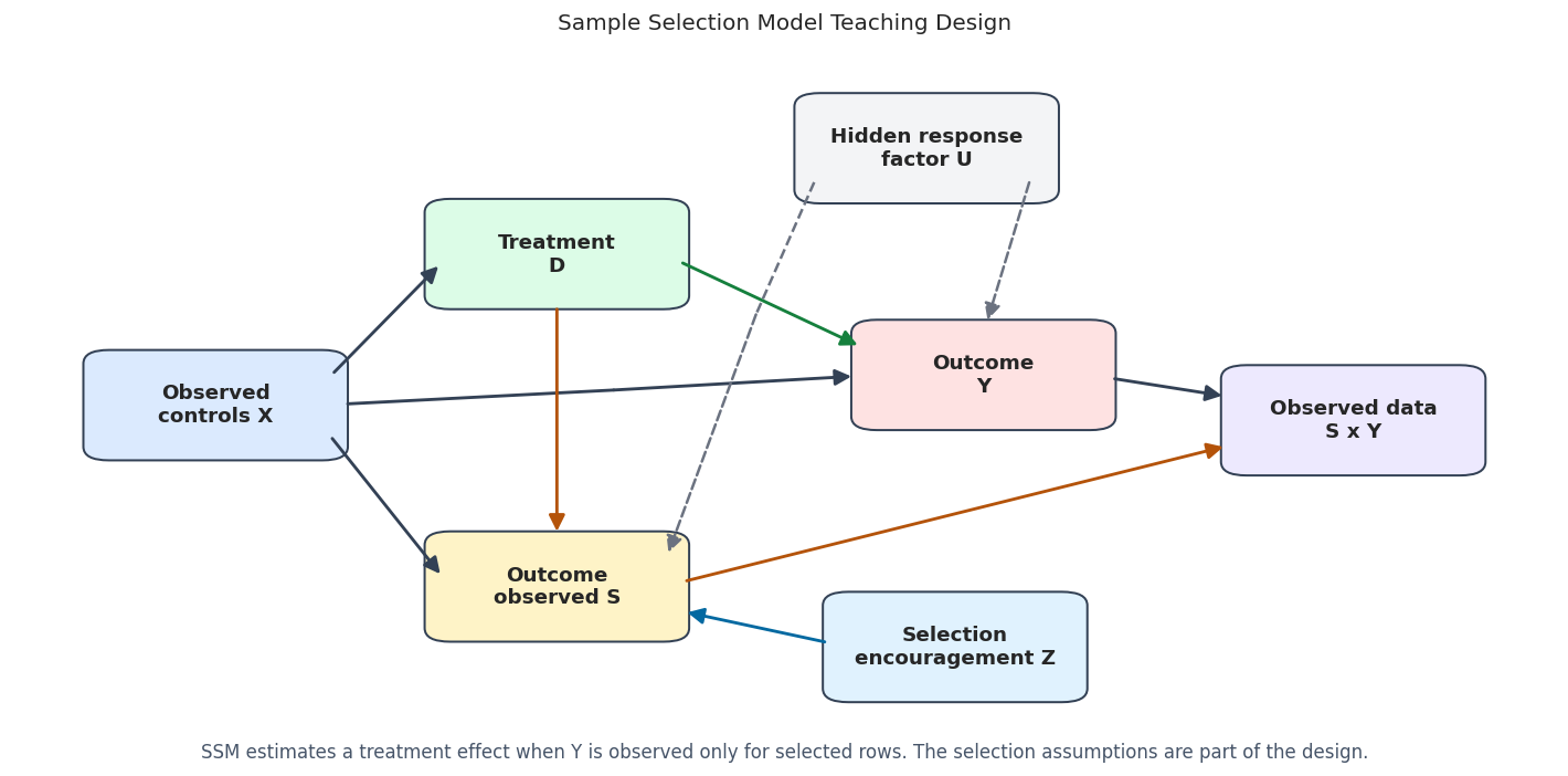
Teaching Diagram

The diagram separates treatment assignment from outcome observation. D determines which potential outcome is relevant. S determines whether we see that outcome. Both can depend on observed controls, and selection can also depend on treatment.

from matplotlib.patches import FancyArrowPatch, FancyBboxPatch

nodes = {
    "X": {"xy": (0.10, 0.54), "label": "Observed\ncontrols X", "color": "#dbeafe"},
    "D": {"xy": (0.34, 0.74), "label": "Treatment\nD", "color": "#dcfce7"},
    "S": {"xy": (0.34, 0.30), "label": "Outcome\nobserved S", "color": "#fef3c7"},
    "Y": {"xy": (0.64, 0.58), "label": "Outcome\nY", "color": "#fee2e2"},
    "Z": {"xy": (0.62, 0.22), "label": "Selection\nencouragement Z", "color": "#e0f2fe"},
    "U": {"xy": (0.60, 0.88), "label": "Hidden response\nfactor U", "color": "#f3f4f6"},
    "O": {"xy": (0.90, 0.52), "label": "Observed data\nS x Y", "color": "#ede9fe"},
}

fig, ax = plt.subplots(figsize=(12, 6))
ax.set_axis_off()
box_w, box_h = 0.15, 0.11
arrow_gap = 0.018


def anchor(node, side):
    x, y = nodes[node]["xy"]
    offsets = {
        "left": (-box_w / 2, 0),
        "right": (box_w / 2, 0),
        "top": (0, box_h / 2),
        "bottom": (0, -box_h / 2),
        "upper_right": (box_w / 2, box_h * 0.25),
        "lower_right": (box_w / 2, -box_h * 0.25),
        "upper_left": (-box_w / 2, box_h * 0.25),
        "lower_left": (-box_w / 2, -box_h * 0.25),
    }
    dx, dy = offsets[side]
    return (x + dx, y + dy)


def shorten_segment(start, end, gap=arrow_gap):
    """Move arrow endpoints inward so arrowheads do not sit on top of boxes."""
    start = np.asarray(start, dtype=float)
    end = np.asarray(end, dtype=float)
    delta = end - start
    length = np.hypot(delta[0], delta[1])
    if length == 0:
        return tuple(start), tuple(end)
    unit = delta / length
    return tuple(start + gap * unit), tuple(end - gap * unit)


def shorten_polyline(points, gap=arrow_gap):
    """Shorten only the first and final endpoints of a routed arrow."""
    pts = [tuple(point) for point in points]
    if len(pts) < 2:
        return pts
    pts[0], _ = shorten_segment(pts[0], pts[1], gap=gap)
    _, pts[-1] = shorten_segment(pts[-2], pts[-1], gap=gap)
    return pts


def draw_arrow(start, end, color, style="solid", rad=0.0, linewidth=1.7, gap=arrow_gap):
    start, end = shorten_segment(start, end, gap=gap)
    arrow = FancyArrowPatch(
        start,
        end,
        arrowstyle="-|>",
        mutation_scale=18,
        linewidth=linewidth,
        color=color,
        linestyle=style,
        shrinkA=0,
        shrinkB=0,
        connectionstyle=f"arc3,rad={rad}",
        zorder=5,
    )
    ax.add_patch(arrow)


def draw_routed_arrow(points, color, style="solid", linewidth=1.7, gap=arrow_gap):
    pts = shorten_polyline(points, gap=gap)
    for start, end in zip(pts[:-2], pts[1:-1]):
        ax.plot([start[0], end[0]], [start[1], end[1]], color=color, linestyle=style, linewidth=linewidth, zorder=5)
    draw_arrow(pts[-2], pts[-1], color=color, style=style, linewidth=linewidth, gap=0.0)

# Main observed paths.
draw_arrow(anchor("X", "upper_right"), anchor("D", "left"), color="#334155")
draw_arrow(anchor("X", "lower_right"), anchor("S", "left"), color="#334155")
draw_routed_arrow([anchor("X", "right"), (0.38, 0.56), anchor("Y", "left")], color="#334155")
draw_arrow(anchor("D", "right"), anchor("Y", "upper_left"), color="#15803d")
draw_arrow(anchor("D", "bottom"), anchor("S", "top"), color="#b45309")
draw_arrow(anchor("Z", "left"), anchor("S", "lower_right"), color="#0369a1")
draw_arrow(anchor("Y", "right"), anchor("O", "upper_left"), color="#334155")
draw_arrow(anchor("S", "right"), anchor("O", "lower_left"), color="#b45309")

# Dashed paths are separated so the nonignorable-selection risk is visible without crossing boxes.
draw_arrow(anchor("U", "lower_right"), anchor("Y", "top"), color="#6b7280", style="dashed", linewidth=1.5)
draw_routed_arrow([anchor("U", "lower_left"), (0.48, 0.66), anchor("S", "upper_right")], color="#6b7280", style="dashed", linewidth=1.5)

for spec in nodes.values():
    x, y = spec["xy"]
    rect = FancyBboxPatch(
        (x - box_w / 2, y - box_h / 2),
        box_w,
        box_h,
        boxstyle="round,pad=0.018",
        facecolor=spec["color"],
        edgecolor="#334155",
        linewidth=1.2,
        zorder=3,
    )
    ax.add_patch(rect)
    ax.text(x, y, spec["label"], ha="center", va="center", fontsize=11, fontweight="bold", zorder=4)

ax.text(
    0.50,
    0.08,
    "SSM estimates a treatment effect when Y is observed only for selected rows. The selection assumptions are part of the design.",
    ha="center",
    va="center",
    fontsize=10,
    color="#475569",
)
ax.set_title("Sample Selection Model Teaching Design", pad=18)
plt.tight_layout()
fig.savefig(FIGURE_DIR / f"{NOTEBOOK_PREFIX}_ssm_design_dag.png", dpi=160, bbox_inches="tight")
plt.show()

The dashed paths show the nonignorable-selection risk. If a hidden response factor affects both outcome observation and the outcome itself, a missing-at-random correction can fail. The selection encouragement Z is useful only if it shifts observation without directly shifting the outcome.

Synthetic Missing-At-Random Data

The first dataset is a missing-at-random design. Selection depends on treatment and observed covariates, including a selection encouragement signal. There is no hidden response factor that directly affects both selection and the outcome.

Because this is synthetic data, we keep a full_outcome column for evaluation. In real selected-outcome data, that full outcome would not be available for unselected rows.

rng = np.random.default_rng(RANDOM_SEED)
N_MAR = 6_000

engagement_score = rng.normal(0, 1, N_MAR)
baseline_value = rng.normal(0, 1, N_MAR)
support_need = rng.normal(0, 1, N_MAR)
prior_usage = rng.normal(0, 1, N_MAR)
mobile_user = rng.binomial(1, 0.48, N_MAR)
selection_encouragement = rng.normal(0, 1, N_MAR)

mar_x = pd.DataFrame(
    {
        "engagement_score": engagement_score,
        "baseline_value": baseline_value,
        "support_need": support_need,
        "prior_usage": prior_usage,
        "mobile_user": mobile_user,
        "selection_encouragement": selection_encouragement,
    }
)
feature_cols_mar = list(mar_x.columns)

true_treatment_propensity = sigmoid(
    -0.10
    + 0.55 * engagement_score
    + 0.35 * baseline_value
    - 0.30 * support_need
    + 0.18 * mobile_user
)
treated = rng.binomial(1, true_treatment_propensity)

true_tau = 1.00 + 0.25 * engagement_score + 0.15 * baseline_value - 0.10 * support_need + 0.08 * mobile_user
mu0 = 3.00 + 0.80 * engagement_score + 0.50 * baseline_value - 0.30 * support_need + 0.25 * prior_usage + 0.20 * mobile_user
full_outcome = mu0 + true_tau * treated + rng.normal(0, 0.70, N_MAR)

true_selection_probability = sigmoid(
    -0.25
    + 0.55 * treated
    + 0.45 * engagement_score
    - 0.55 * support_need
    + 0.25 * prior_usage
    + 0.70 * selection_encouragement
)
selected = rng.binomial(1, true_selection_probability)

# DoubleMLSSM expects a numeric outcome column for every row. The selection indicator tells the estimator
# which outcomes are genuinely observed and should enter the selected-outcome regressions.
outcome_observed = full_outcome.copy()
outcome_observed[selected == 0] = 0.0

mar_df = pd.concat(
    [
        pd.DataFrame({"row_id": np.arange(N_MAR)}),
        mar_x,
        pd.DataFrame(
            {
                "treated": treated,
                "selected": selected,
                "outcome_observed": outcome_observed,
                "full_outcome": full_outcome,
                "true_tau": true_tau,
                "true_treatment_propensity": true_treatment_propensity,
                "true_selection_probability": true_selection_probability,
            }
        ),
    ],
    axis=1,
)

TRUE_MAR_ATE = mar_df["true_tau"].mean()
TRUE_MAR_ATT = mar_df.loc[mar_df["treated"] == 1, "true_tau"].mean()

mar_path = DATASET_DIR / f"{NOTEBOOK_PREFIX}_synthetic_mar_selection_data.csv"
mar_df.to_csv(mar_path, index=False)

print(f"Rows: {len(mar_df):,}")
print(f"Selected share: {mar_df['selected'].mean():.3f}")
print(f"True MAR ATE: {TRUE_MAR_ATE:.4f}")
print(f"True MAR ATT: {TRUE_MAR_ATT:.4f}")
print(f"Saved data to: {mar_path.relative_to(PROJECT_ROOT)}")
display(mar_df.head())
Rows: 6,000
Selected share: 0.518
True MAR ATE: 1.0323
True MAR ATT: 1.1265
Saved data to: notebooks/tutorials/doubleml/outputs/datasets/08_synthetic_mar_selection_data.csv
row_id engagement_score baseline_value support_need prior_usage mobile_user selection_encouragement treated selected outcome_observed full_outcome true_tau true_treatment_propensity true_selection_probability
0 0 0.304717 0.225117 -0.309788 0.636265 0 0.178007 1 0 0.000000 3.855320 1.140926 0.559546 0.709133
1 1 -1.039984 -0.053343 0.060236 1.579594 1 0.177642 1 1 2.795688 2.795688 0.805979 0.370813 0.578867
2 2 0.750451 0.864044 -1.240756 -0.668791 1 0.985953 1 1 6.691277 6.691277 1.521295 0.762673 0.863314
3 3 0.940565 0.606733 -1.387754 -0.545453 0 -0.306807 1 1 6.255977 6.255977 1.464927 0.740005 0.756832
4 4 -1.951035 -2.985823 0.182298 -0.208867 1 0.442759 1 0 0.000000 1.885728 0.126138 0.109799 0.396394

The selected share is neither tiny nor near one, so the notebook has enough observed and unobserved rows to show the selection problem. The target for DoubleMLSSM is the ATE over the full population, not just the selected rows.

Field Dictionary

A field dictionary is especially important for selected-outcome problems because it prevents a common mistake: treating the selection indicator as an ordinary covariate or dropping unselected rows before the selection model is built.

mar_field_dictionary = pd.DataFrame(
    [
        {"field": "row_id", "role": "identifier", "description": "Unique row identifier."},
        {"field": "treated", "role": "treatment", "description": "Binary treatment indicator D."},
        {"field": "selected", "role": "selection indicator", "description": "Equals 1 if the outcome is observed."},
        {"field": "outcome_observed", "role": "observed outcome", "description": "Outcome column passed to DoubleMLSSM; unselected rows are filled with 0 and marked by selected=0."},
        {"field": "full_outcome", "role": "simulation truth", "description": "Outcome for every row, kept only because this is synthetic data."},
        {"field": "engagement_score", "role": "covariate", "description": "Observed pre-treatment feature related to treatment, selection, and outcome."},
        {"field": "baseline_value", "role": "covariate", "description": "Observed baseline outcome predictor."},
        {"field": "support_need", "role": "covariate", "description": "Observed need/risk feature."},
        {"field": "prior_usage", "role": "covariate", "description": "Observed prior activity signal."},
        {"field": "mobile_user", "role": "covariate", "description": "Observed binary segment marker."},
        {"field": "selection_encouragement", "role": "covariate in MAR design", "description": "Observed signal that predicts outcome observation."},
        {"field": "true_tau", "role": "simulation truth", "description": "Individual treatment effect."},
        {"field": "true_treatment_propensity", "role": "simulation truth", "description": "True P(D=1|X)."},
        {"field": "true_selection_probability", "role": "simulation truth", "description": "True P(S=1|D,X)."},
    ]
)
save_table(mar_field_dictionary, f"{NOTEBOOK_PREFIX}_mar_field_dictionary.csv")
display(mar_field_dictionary)
field role description
0 row_id identifier Unique row identifier.
1 treated treatment Binary treatment indicator D.
2 selected selection indicator Equals 1 if the outcome is observed.
3 outcome_observed observed outcome Outcome column passed to DoubleMLSSM; unselect...
4 full_outcome simulation truth Outcome for every row, kept only because this ...
5 engagement_score covariate Observed pre-treatment feature related to trea...
6 baseline_value covariate Observed baseline outcome predictor.
7 support_need covariate Observed need/risk feature.
8 prior_usage covariate Observed prior activity signal.
9 mobile_user covariate Observed binary segment marker.
10 selection_encouragement covariate in MAR design Observed signal that predicts outcome observat...
11 true_tau simulation truth Individual treatment effect.
12 true_treatment_propensity simulation truth True P(D=1|X).
13 true_selection_probability simulation truth True P(S=1|D,X).

Notice that selected is not part of the ordinary feature list. It has a special role through s_col, because it determines which outcomes are observed.

Data Audit

Before fitting a sample-selection model, check selection rate, treatment rate, selected-by-treatment cells, and missingness. The selection cells matter because outcome models are trained only where S = 1 within treatment arms.

mar_audit = pd.DataFrame(
    [
        {"metric": "rows", "value": len(mar_df)},
        {"metric": "columns", "value": mar_df.shape[1]},
        {"metric": "missing_cells", "value": int(mar_df.isna().sum().sum())},
        {"metric": "treated_share", "value": mar_df["treated"].mean()},
        {"metric": "selected_share", "value": mar_df["selected"].mean()},
        {"metric": "selected_share_treated", "value": mar_df.loc[mar_df["treated"] == 1, "selected"].mean()},
        {"metric": "selected_share_control", "value": mar_df.loc[mar_df["treated"] == 0, "selected"].mean()},
        {"metric": "true_ate", "value": TRUE_MAR_ATE},
    ]
)
mar_cell_counts = mar_df.groupby(["treated", "selected"]).size().rename("n").reset_index()
save_table(mar_audit, f"{NOTEBOOK_PREFIX}_mar_data_audit.csv")
save_table(mar_cell_counts, f"{NOTEBOOK_PREFIX}_mar_treatment_selection_cells.csv")
display(mar_audit)
display(mar_cell_counts)
metric value
0 rows 6000.000000
1 columns 14.000000
2 missing_cells 0.000000
3 treated_share 0.492167
4 selected_share 0.518333
5 selected_share_treated 0.617338
6 selected_share_control 0.422383
7 true_ate 1.032326
treated selected n
0 0 0 1760
1 0 1 1287
2 1 0 1130
3 1 1 1823

Every treatment-selection cell has enough rows. If selected treated rows or selected control rows were rare, the outcome nuisance functions g(1, X) or g(0, X) would be weak.

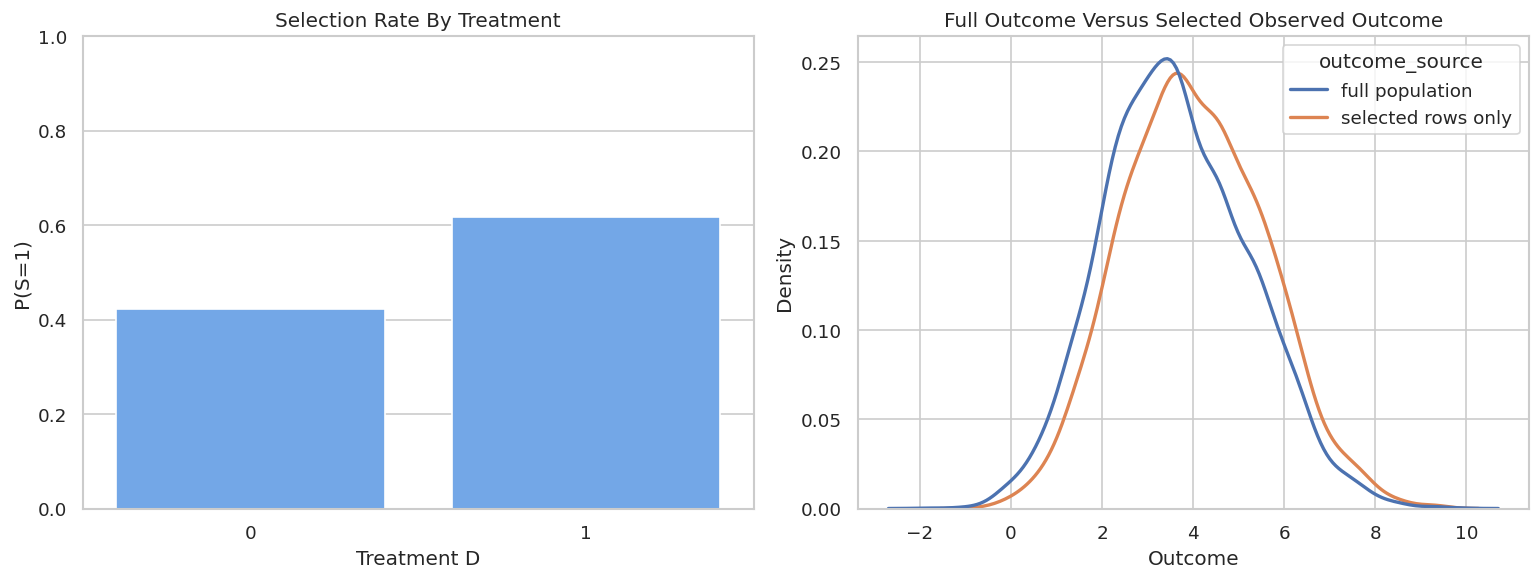
Selection Rates And Outcome Visibility

The next plot shows two different facts at once: selected shares differ by treatment status, and observed selected outcomes differ from the full outcome distribution. In real data, the full distribution would be hidden, which is exactly why the design assumption matters.

selection_rate = (
    mar_df.groupby("treated")
    .agg(selected_rate=("selected", "mean"), n=("selected", "size"))
    .reset_index()
)

plot_outcomes = pd.concat(
    [
        mar_df.assign(outcome_source="full population", outcome_for_plot=mar_df["full_outcome"]),
        mar_df.loc[mar_df["selected"] == 1].assign(
            outcome_source="selected rows only",
            outcome_for_plot=mar_df.loc[mar_df["selected"] == 1, "outcome_observed"],
        ),
    ],
    ignore_index=True,
)

fig, axes = plt.subplots(1, 2, figsize=(13, 5))
sns.barplot(data=selection_rate, x="treated", y="selected_rate", color="#60a5fa", ax=axes[0])
axes[0].set_title("Selection Rate By Treatment")
axes[0].set_xlabel("Treatment D")
axes[0].set_ylabel("P(S=1)")
axes[0].set_ylim(0, 1)

sns.kdeplot(
    data=plot_outcomes,
    x="outcome_for_plot",
    hue="outcome_source",
    common_norm=False,
    linewidth=2,
    ax=axes[1],
)
axes[1].set_title("Full Outcome Versus Selected Observed Outcome")
axes[1].set_xlabel("Outcome")
axes[1].set_ylabel("Density")

plt.tight_layout()
fig.savefig(FIGURE_DIR / f"{NOTEBOOK_PREFIX}_mar_selection_and_outcome_visibility.png", dpi=160, bbox_inches="tight")
plt.show()

display(selection_rate)

treated selected_rate n
0 0 0.422383 3047
1 1 0.617338 2953

Treatment affects selection, and selected rows have a shifted outcome distribution. A selected-row-only analysis is therefore risky because it changes the population being analyzed.

Covariate Balance And Selection Balance

Selection can distort the covariate distribution. The table below compares selected and unselected rows on observed features. Large differences do not make correction impossible, but they make the selection model more important.

balance_rows = []
for col in feature_cols_mar:
    selected_mean = mar_df.loc[mar_df["selected"] == 1, col].mean()
    unselected_mean = mar_df.loc[mar_df["selected"] == 0, col].mean()
    pooled_sd = mar_df[col].std(ddof=1)
    balance_rows.append(
        {
            "feature": col,
            "selected_mean": selected_mean,
            "unselected_mean": unselected_mean,
            "difference": selected_mean - unselected_mean,
            "standardized_difference": (selected_mean - unselected_mean) / pooled_sd,
        }
    )

selection_balance = pd.DataFrame(balance_rows).sort_values("standardized_difference", key=np.abs, ascending=False)
save_table(selection_balance, f"{NOTEBOOK_PREFIX}_mar_selection_covariate_balance.csv")
display(selection_balance)
feature selected_mean unselected_mean difference standardized_difference
5 selection_encouragement 0.279948 -0.288673 0.568620 0.567095
2 support_need -0.208256 0.262695 -0.470952 -0.470948
0 engagement_score 0.198322 -0.230804 0.429127 0.427795
3 prior_usage 0.109263 -0.048825 0.158088 0.158684
1 baseline_value -0.010164 -0.020088 0.009924 0.009853
4 mobile_user 0.483280 0.479585 0.003695 0.007394

The selected sample is not a random slice of the full sample. The encouragement and support-need variables are especially important for modeling selection.

Naive Baselines

The first baseline uses only selected rows and compares treated versus control outcomes. The second baseline uses the synthetic full outcome and is shown only for teaching. In real selected-outcome data, the second baseline cannot be computed.

selected_df = mar_df.loc[mar_df["selected"] == 1].copy()

naive_selected_diff = (
    selected_df.loc[selected_df["treated"] == 1, "outcome_observed"].mean()
    - selected_df.loc[selected_df["treated"] == 0, "outcome_observed"].mean()
)
full_population_diff = (
    mar_df.loc[mar_df["treated"] == 1, "full_outcome"].mean()
    - mar_df.loc[mar_df["treated"] == 0, "full_outcome"].mean()
)

selected_ols = smf.ols(
    formula="outcome_observed ~ treated + " + " + ".join(feature_cols_mar),
    data=selected_df,
).fit(cov_type="HC3")

baseline_summary = pd.DataFrame(
    [
        {
            "estimator": "Selected-row treated-control difference",
            "theta_hat": naive_selected_diff,
            "std_error": np.nan,
            "ci_95_lower": np.nan,
            "ci_95_upper": np.nan,
            "true_target": TRUE_MAR_ATE,
            "bias_vs_target": naive_selected_diff - TRUE_MAR_ATE,
        },
        {
            "estimator": "Synthetic full-population treated-control difference",
            "theta_hat": full_population_diff,
            "std_error": np.nan,
            "ci_95_lower": np.nan,
            "ci_95_upper": np.nan,
            "true_target": TRUE_MAR_ATE,
            "bias_vs_target": full_population_diff - TRUE_MAR_ATE,
        },
        {
            "estimator": "Selected-row OLS with covariates",
            "theta_hat": float(selected_ols.params["treated"]),
            "std_error": float(selected_ols.bse["treated"]),
            "ci_95_lower": float(selected_ols.conf_int().loc["treated", 0]),
            "ci_95_upper": float(selected_ols.conf_int().loc["treated", 1]),
            "true_target": TRUE_MAR_ATE,
            "bias_vs_target": float(selected_ols.params["treated"] - TRUE_MAR_ATE),
        },
    ]
)
save_table(baseline_summary, f"{NOTEBOOK_PREFIX}_mar_baseline_estimates.csv")
display(baseline_summary)
estimator theta_hat std_error ci_95_lower ci_95_upper true_target bias_vs_target
0 Selected-row treated-control difference 1.675867 NaN NaN NaN 1.032326 0.643540
1 Synthetic full-population treated-control diff... 1.732946 NaN NaN NaN 1.032326 0.700620
2 Selected-row OLS with covariates 1.065852 0.026952 1.013027 1.118678 1.032326 0.033526

The selected-row difference is far from the true ATE because it mixes treatment assignment, treatment heterogeneity, and outcome observation. Covariate adjustment helps, but it still does not explicitly model the missing-outcome process for the full target population.

Manual Cross-Fitted MAR Score

Before fitting DoubleMLSSM, we compute a small manual missing-at-random score. This makes the mechanics visible.

The code trains:

  • g(1, X) on selected treated rows;
  • g(0, X) on selected control rows;
  • pi(D, X) on all rows to predict selection;
  • m(X) on all rows to predict treatment.

Then it combines residualized observed outcomes with outcome-model predictions.

def crossfit_mar_ssm(df, y_col, d_col, s_col, x_cols, ml_g, ml_pi, ml_m, n_splits=5, seed=RANDOM_SEED):
    X = df[x_cols].reset_index(drop=True)
    y = df[y_col].to_numpy()
    d = df[d_col].to_numpy()
    s = df[s_col].to_numpy()
    dx = pd.concat([X, pd.Series(d, name=d_col)], axis=1)
    n = len(df)

    g1_hat = np.full(n, np.nan)
    g0_hat = np.full(n, np.nan)
    pi_hat = np.full(n, np.nan)
    m_hat = np.full(n, np.nan)

    strata = d + 2 * s
    splitter = StratifiedKFold(n_splits=n_splits, shuffle=True, random_state=seed)

    for train_idx, test_idx in splitter.split(X, strata):
        train_selected_treated = train_idx[(s[train_idx] == 1) & (d[train_idx] == 1)]
        train_selected_control = train_idx[(s[train_idx] == 1) & (d[train_idx] == 0)]

        g1_model = clone(ml_g)
        g0_model = clone(ml_g)
        pi_model = clone(ml_pi)
        m_model = clone(ml_m)

        g1_model.fit(X.iloc[train_selected_treated], y[train_selected_treated])
        g0_model.fit(X.iloc[train_selected_control], y[train_selected_control])
        pi_model.fit(dx.iloc[train_idx], s[train_idx])
        m_model.fit(X.iloc[train_idx], d[train_idx])

        g1_hat[test_idx] = g1_model.predict(X.iloc[test_idx])
        g0_hat[test_idx] = g0_model.predict(X.iloc[test_idx])
        pi_hat[test_idx] = predict_probability(pi_model, dx.iloc[test_idx])
        m_hat[test_idx] = predict_probability(m_model, X.iloc[test_idx])

    pi_hat = clip_probability(pi_hat)
    m_hat = clip_probability(m_hat)

    treated_contribution = d * s * (y - g1_hat) / (m_hat * pi_hat) + g1_hat
    control_contribution = (1 - d) * s * (y - g0_hat) / ((1 - m_hat) * pi_hat) + g0_hat
    score_contribution = treated_contribution - control_contribution

    theta_hat = score_contribution.mean()
    std_error = score_contribution.std(ddof=1) / np.sqrt(n)

    summary = pd.DataFrame(
        [
            {
                "estimator": "Manual cross-fitted MAR SSM",
                "theta_hat": theta_hat,
                "std_error": std_error,
                "ci_95_lower": theta_hat - 1.96 * std_error,
                "ci_95_upper": theta_hat + 1.96 * std_error,
                "true_target": TRUE_MAR_ATE,
                "bias_vs_target": theta_hat - TRUE_MAR_ATE,
            }
        ]
    )
    diagnostics = pd.DataFrame(
        {
            "g1_hat": g1_hat,
            "g0_hat": g0_hat,
            "pi_hat": pi_hat,
            "m_hat": m_hat,
            "score_contribution": score_contribution,
            "treated": d,
            "selected": s,
        }
    )
    return summary, diagnostics

linear_g, linear_pi, linear_m = make_linear_learners()
manual_mar_summary, manual_mar_diagnostics = crossfit_mar_ssm(
    mar_df,
    y_col="outcome_observed",
    d_col="treated",
    s_col="selected",
    x_cols=feature_cols_mar,
    ml_g=linear_g,
    ml_pi=linear_pi,
    ml_m=linear_m,
    n_splits=5,
    seed=RANDOM_SEED,
)
save_table(manual_mar_summary, f"{NOTEBOOK_PREFIX}_manual_mar_ssm_summary.csv")
save_table(manual_mar_diagnostics.describe().reset_index(), f"{NOTEBOOK_PREFIX}_manual_mar_ssm_diagnostics.csv")
display(manual_mar_summary)
estimator theta_hat std_error ci_95_lower ci_95_upper true_target bias_vs_target
0 Manual cross-fitted MAR SSM 1.003513 0.030544 0.943647 1.06338 1.032326 -0.028813

The manual score is much closer to the true ATE than the selected-row difference. That is the core lesson: selection correction uses unselected rows through the selection and treatment models, even though their outcomes are not observed.

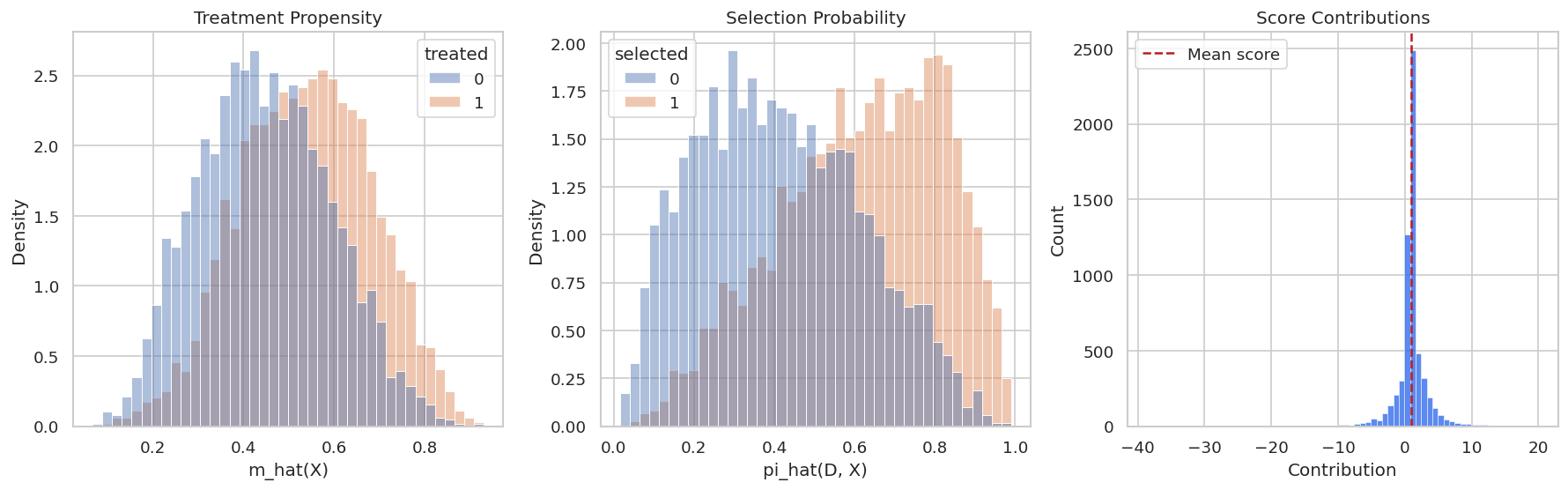
Manual Score Diagnostics

The manual diagnostics check whether treatment and selection probabilities are extreme. The score contribution plot shows whether a few rows dominate the estimate.

fig, axes = plt.subplots(1, 3, figsize=(15, 4.8))

sns.histplot(
    data=manual_mar_diagnostics,
    x="m_hat",
    hue="treated",
    bins=40,
    stat="density",
    common_norm=False,
    alpha=0.45,
    ax=axes[0],
)
axes[0].set_title("Treatment Propensity")
axes[0].set_xlabel("m_hat(X)")
axes[0].set_ylabel("Density")

sns.histplot(
    data=manual_mar_diagnostics,
    x="pi_hat",
    hue="selected",
    bins=40,
    stat="density",
    common_norm=False,
    alpha=0.45,
    ax=axes[1],
)
axes[1].set_title("Selection Probability")
axes[1].set_xlabel("pi_hat(D, X)")
axes[1].set_ylabel("Density")

sns.histplot(
    data=manual_mar_diagnostics,
    x="score_contribution",
    bins=70,
    color="#2563eb",
    ax=axes[2],
)
axes[2].axvline(manual_mar_summary["theta_hat"].iloc[0], color="#b91c1c", linestyle="--", label="Mean score")
axes[2].set_title("Score Contributions")
axes[2].set_xlabel("Contribution")
axes[2].set_ylabel("Count")
axes[2].legend()

plt.tight_layout()
fig.savefig(FIGURE_DIR / f"{NOTEBOOK_PREFIX}_manual_mar_score_diagnostics.png", dpi=160, bbox_inches="tight")
plt.show()

The treatment and selection predictions are mostly away from 0 and 1. That matters because inverse-probability terms become unstable when predicted probabilities are too small.

DoubleML Sample-Selection Backend

DoubleMLSSMData is the data contract for sample-selection models. The selection column is passed as s_col. Unselected rows stay in the data because they are needed for the treatment and selection nuisance models.

mar_dml_data = DoubleMLSSMData(
    mar_df,
    y_col="outcome_observed",
    d_cols="treated",
    s_col="selected",
    x_cols=feature_cols_mar,
)

mar_backend_summary = pd.DataFrame(
    [
        {"property": "n_obs", "value": mar_dml_data.n_obs},
        {"property": "outcome", "value": mar_dml_data.y_col},
        {"property": "treatment", "value": ", ".join(mar_dml_data.d_cols)},
        {"property": "selection", "value": mar_dml_data.s_col},
        {"property": "n_covariates", "value": len(mar_dml_data.x_cols)},
        {"property": "covariates", "value": ", ".join(mar_dml_data.x_cols)},
    ]
)
save_table(mar_backend_summary, f"{NOTEBOOK_PREFIX}_mar_doublemlssm_backend.csv")
display(mar_backend_summary)
property value
0 n_obs 6000
1 outcome outcome_observed
2 treatment treated
3 selection selected
4 n_covariates 6
5 covariates engagement_score, baseline_value, support_need...

This is the most important API cell in the notebook. If s_col is missing, the model no longer knows which outcomes are observed and the selected-outcome design is lost.

Fit DoubleMLSSM Under Missing At Random

We fit three versions:

  • linear nuisance learners;
  • gradient boosting nuisance learners;
  • gradient boosting with normalized inverse-probability weights.

The normalized version can be helpful when weights are noisy, but it is not a magic fix for poor overlap or wrong assumptions.

mar_model_rows = []
mar_models = {}

ml_g_linear, ml_pi_linear, ml_m_linear = make_linear_learners()
mar_ssm_linear = DoubleMLSSM(
    mar_dml_data,
    ml_g=ml_g_linear,
    ml_pi=ml_pi_linear,
    ml_m=ml_m_linear,
    n_folds=5,
    score="missing-at-random",
)
mar_ssm_linear.fit(store_predictions=True)
mar_models["MAR linear"] = mar_ssm_linear
mar_model_rows.append(summarize_doubleml(mar_ssm_linear, "MAR linear", "missing-at-random", TRUE_MAR_ATE))

ml_g_hgb, ml_pi_hgb, ml_m_hgb = make_hgb_learners(seed=RANDOM_SEED + 10, max_iter=90)
mar_ssm_hgb = DoubleMLSSM(
    mar_dml_data,
    ml_g=ml_g_hgb,
    ml_pi=ml_pi_hgb,
    ml_m=ml_m_hgb,
    n_folds=5,
    score="missing-at-random",
)
mar_ssm_hgb.fit(store_predictions=True)
mar_models["MAR HGB"] = mar_ssm_hgb
mar_model_rows.append(summarize_doubleml(mar_ssm_hgb, "MAR HGB", "missing-at-random", TRUE_MAR_ATE))

ml_g_norm, ml_pi_norm, ml_m_norm = make_hgb_learners(seed=RANDOM_SEED + 20, max_iter=90)
mar_ssm_hgb_norm = DoubleMLSSM(
    mar_dml_data,
    ml_g=ml_g_norm,
    ml_pi=ml_pi_norm,
    ml_m=ml_m_norm,
    n_folds=5,
    score="missing-at-random",
    normalize_ipw=True,
)
mar_ssm_hgb_norm.fit(store_predictions=True)
mar_models["MAR HGB normalized IPW"] = mar_ssm_hgb_norm
mar_model_rows.append(summarize_doubleml(mar_ssm_hgb_norm, "MAR HGB normalized IPW", "missing-at-random", TRUE_MAR_ATE))

mar_doubleml_summary = pd.DataFrame(mar_model_rows)
save_table(mar_doubleml_summary, f"{NOTEBOOK_PREFIX}_mar_doublemlssm_summary.csv")
display(mar_doubleml_summary)
estimator design theta_hat std_error ci_95_lower ci_95_upper true_target bias_vs_target
0 MAR linear missing-at-random 1.001539 0.030564 0.941634 1.061444 1.032326 -0.030787
1 MAR HGB missing-at-random 1.002785 0.036305 0.931628 1.073943 1.032326 -0.029541
2 MAR HGB normalized IPW missing-at-random 1.023998 0.016952 0.990773 1.057222 1.032326 -0.008329

The DoubleML estimates are close to the true full-population ATE. The selected-row difference was much larger, which shows why the selection problem matters.
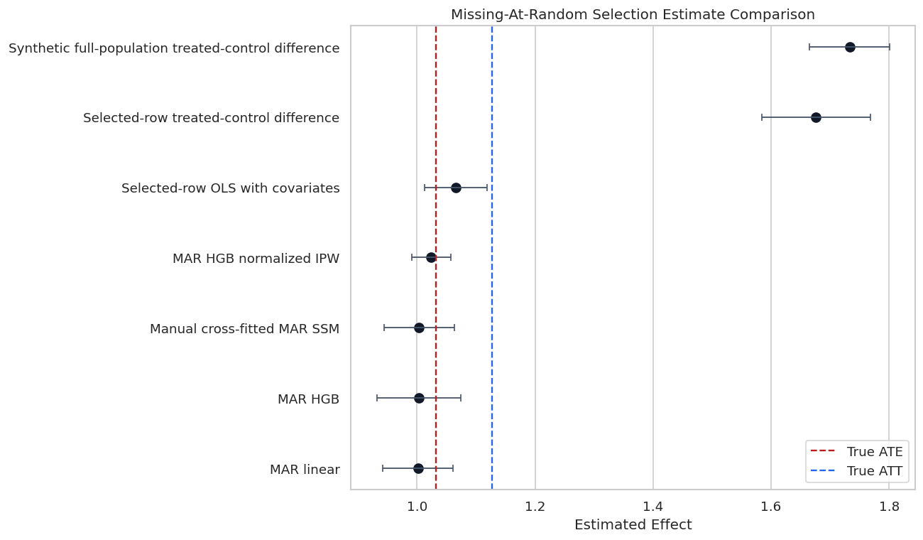
Estimate Comparison

The comparison plot puts the naive baselines, manual score, and DoubleML estimates on one axis. This is often the clearest way to communicate what selection correction changed.

mar_estimates = pd.concat(
    [
        baseline_summary,
        manual_mar_summary,
        mar_doubleml_summary,
    ],
    ignore_index=True,
    sort=False,
)

# Add simple intervals for rows without model-based intervals when available.
selected_diff_se = np.sqrt(
    selected_df.loc[selected_df["treated"] == 1, "outcome_observed"].var(ddof=1) / (selected_df["treated"] == 1).sum()
    + selected_df.loc[selected_df["treated"] == 0, "outcome_observed"].var(ddof=1) / (selected_df["treated"] == 0).sum()
)
mar_estimates.loc[mar_estimates["estimator"] == "Selected-row treated-control difference", "std_error"] = selected_diff_se
mar_estimates.loc[mar_estimates["estimator"] == "Selected-row treated-control difference", "ci_95_lower"] = naive_selected_diff - 1.96 * selected_diff_se
mar_estimates.loc[mar_estimates["estimator"] == "Selected-row treated-control difference", "ci_95_upper"] = naive_selected_diff + 1.96 * selected_diff_se

full_diff_se = np.sqrt(
    mar_df.loc[mar_df["treated"] == 1, "full_outcome"].var(ddof=1) / (mar_df["treated"] == 1).sum()
    + mar_df.loc[mar_df["treated"] == 0, "full_outcome"].var(ddof=1) / (mar_df["treated"] == 0).sum()
)
mar_estimates.loc[mar_estimates["estimator"] == "Synthetic full-population treated-control difference", "std_error"] = full_diff_se
mar_estimates.loc[mar_estimates["estimator"] == "Synthetic full-population treated-control difference", "ci_95_lower"] = full_population_diff - 1.96 * full_diff_se
mar_estimates.loc[mar_estimates["estimator"] == "Synthetic full-population treated-control difference", "ci_95_upper"] = full_population_diff + 1.96 * full_diff_se

save_table(mar_estimates, f"{NOTEBOOK_PREFIX}_mar_estimate_comparison.csv")
plot_mar_estimates = add_ci_columns(mar_estimates)

fig, ax = plt.subplots(figsize=(11, 6.5))
order = plot_mar_estimates.sort_values("theta_hat", ascending=False)["estimator"]
sns.pointplot(
    data=plot_mar_estimates,
    y="estimator",
    x="theta_hat",
    order=order,
    linestyle="none",
    color="#111827",
    errorbar=None,
    ax=ax,
)
for y_pos, (_, row) in enumerate(plot_mar_estimates.set_index("estimator").loc[order].reset_index().iterrows()):
    ax.errorbar(
        x=row["theta_hat"],
        y=y_pos,
        xerr=[[row["lower_error"]], [row["upper_error"]]],
        fmt="none",
        color="#475569",
        capsize=3,
        linewidth=1.1,
    )
ax.axvline(TRUE_MAR_ATE, color="#b91c1c", linestyle="--", linewidth=1.4, label="True ATE")
ax.axvline(TRUE_MAR_ATT, color="#2563eb", linestyle="--", linewidth=1.4, label="True ATT")
ax.set_title("Missing-At-Random Selection Estimate Comparison")
ax.set_xlabel("Estimated Effect")
ax.set_ylabel("")
ax.legend(loc="best")
plt.tight_layout()
fig.savefig(FIGURE_DIR / f"{NOTEBOOK_PREFIX}_mar_estimate_comparison.png", dpi=160, bbox_inches="tight")
plt.show()

display(mar_estimates)

estimator theta_hat std_error ci_95_lower ci_95_upper true_target bias_vs_target design
0 Selected-row treated-control difference 1.675867 0.046957 1.583831 1.767903 1.032326 0.643540 NaN
1 Synthetic full-population treated-control diff... 1.732946 0.034447 1.665431 1.800462 1.032326 0.700620 NaN
2 Selected-row OLS with covariates 1.065852 0.026952 1.013027 1.118678 1.032326 0.033526 NaN
3 Manual cross-fitted MAR SSM 1.003513 0.030544 0.943647 1.063380 1.032326 -0.028813 NaN
4 MAR linear 1.001539 0.030564 0.941634 1.061444 1.032326 -0.030787 missing-at-random
5 MAR HGB 1.002785 0.036305 0.931628 1.073943 1.032326 -0.029541 missing-at-random
6 MAR HGB normalized IPW 1.023998 0.016952 0.990773 1.057222 1.032326 -0.008329 missing-at-random

The corrected estimates move toward the full-population ATE. The plot also shows that the ATT is a different target; selected-outcome correction does not remove the need to state the estimand.

Nuisance Learner Diagnostics

Now we inspect the nuisance learners. These diagnostics are not a proof of selection validity. They are checks that the prediction components are not obviously broken.

mar_loss_tables = []
for label, model in mar_models.items():
    mar_loss_tables.append(learner_loss_table(model, label))

mar_nuisance_losses = pd.concat(mar_loss_tables, ignore_index=True)
save_table(mar_nuisance_losses, f"{NOTEBOOK_PREFIX}_mar_nuisance_losses.csv")
display(mar_nuisance_losses)
model learner metric_value metric
0 MAR linear ml_g_d0 2.238000 RMSE for outcome learners; classification erro...
1 MAR linear ml_g_d1 2.837962 RMSE for outcome learners; classification erro...
2 MAR linear ml_pi 0.446393 RMSE for outcome learners; classification erro...
3 MAR linear ml_m 0.476925 RMSE for outcome learners; classification erro...
4 MAR HGB ml_g_d0 2.252895 RMSE for outcome learners; classification erro...
5 MAR HGB ml_g_d1 2.862023 RMSE for outcome learners; classification erro...
6 MAR HGB ml_pi 0.448827 RMSE for outcome learners; classification erro...
7 MAR HGB ml_m 0.480633 RMSE for outcome learners; classification erro...
8 MAR HGB normalized IPW ml_g_d0 2.245353 RMSE for outcome learners; classification erro...
9 MAR HGB normalized IPW ml_g_d1 2.863304 RMSE for outcome learners; classification erro...
10 MAR HGB normalized IPW ml_pi 0.449762 RMSE for outcome learners; classification erro...
11 MAR HGB normalized IPW ml_m 0.482784 RMSE for outcome learners; classification erro...

The outcome nuisance losses are measured on the outcome scale. The propensity learner losses summarize classification-style performance. If these losses were very poor, the final estimate would deserve more skepticism.

Prediction Quality Against Synthetic Truth

Because the data are synthetic, we can compare the HGB nuisance predictions to true treatment and selection probabilities. In real data, this truth is unavailable, but the same plots can still reveal extreme probabilities.

mar_hgb_predictions = pd.DataFrame(
    {
        "treated": mar_df["treated"],
        "selected": mar_df["selected"],
        "true_treatment_propensity": mar_df["true_treatment_propensity"],
        "true_selection_probability": mar_df["true_selection_probability"],
        "m_hat": prediction_vector(mar_ssm_hgb, "ml_m"),
        "pi_hat": prediction_vector(mar_ssm_hgb, "ml_pi"),
        "g0_hat": prediction_vector(mar_ssm_hgb, "ml_g_d0"),
        "g1_hat": prediction_vector(mar_ssm_hgb, "ml_g_d1"),
        "full_outcome": mar_df["full_outcome"],
        "true_tau": mar_df["true_tau"],
    }
)

mar_prediction_quality = pd.DataFrame(
    [
        {
            "quantity": "treatment propensity m_hat",
            "rmse_vs_truth": rmse(mar_hgb_predictions["true_treatment_propensity"], mar_hgb_predictions["m_hat"]),
            "mae_vs_truth": mean_absolute_error(mar_hgb_predictions["true_treatment_propensity"], mar_hgb_predictions["m_hat"]),
        },
        {
            "quantity": "selection probability pi_hat",
            "rmse_vs_truth": rmse(mar_hgb_predictions["true_selection_probability"], mar_hgb_predictions["pi_hat"]),
            "mae_vs_truth": mean_absolute_error(mar_hgb_predictions["true_selection_probability"], mar_hgb_predictions["pi_hat"]),
        },
    ]
)
save_table(mar_prediction_quality, f"{NOTEBOOK_PREFIX}_mar_hgb_prediction_quality.csv")
display(mar_prediction_quality)
quantity rmse_vs_truth mae_vs_truth
0 treatment propensity m_hat 0.072886 0.057121
1 selection probability pi_hat 0.073758 0.056554

The probability predictions track the synthetic truth reasonably well. This does not guarantee a causal estimate, but it confirms that the nuisance models are learning the intended observed structure.

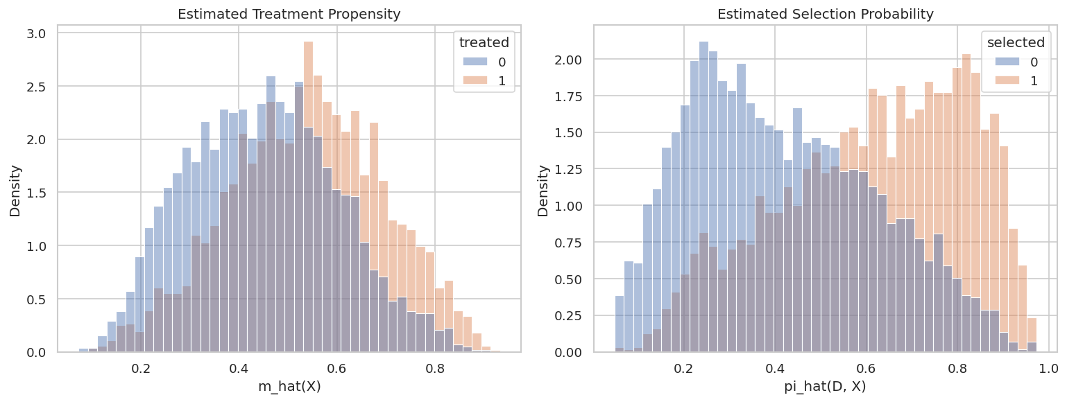
Treatment And Selection Overlap

The next plot is one of the most important diagnostics in a sample-selection analysis. Both the treatment propensity and the selection probability appear in denominators. Near-zero probabilities can create unstable weights.

fig, axes = plt.subplots(1, 2, figsize=(13, 5))

sns.histplot(
    data=mar_hgb_predictions,
    x="m_hat",
    hue="treated",
    bins=45,
    stat="density",
    common_norm=False,
    alpha=0.45,
    ax=axes[0],
)
axes[0].set_title("Estimated Treatment Propensity")
axes[0].set_xlabel("m_hat(X)")
axes[0].set_ylabel("Density")

sns.histplot(
    data=mar_hgb_predictions,
    x="pi_hat",
    hue="selected",
    bins=45,
    stat="density",
    common_norm=False,
    alpha=0.45,
    ax=axes[1],
)
axes[1].set_title("Estimated Selection Probability")
axes[1].set_xlabel("pi_hat(D, X)")
axes[1].set_ylabel("Density")

plt.tight_layout()
fig.savefig(FIGURE_DIR / f"{NOTEBOOK_PREFIX}_mar_overlap_diagnostics.png", dpi=160, bbox_inches="tight")
plt.show()

The predicted probabilities have usable overlap and are not concentrated at the clipping boundaries. That is a good sign for this synthetic example.

Bootstrap Confidence Interval

The multiplier bootstrap gives another uncertainty view for the preferred MAR model. It quantifies sampling uncertainty under the maintained design assumptions.

mar_ssm_hgb.bootstrap(method="normal", n_rep_boot=500)
mar_bootstrap_ci = mar_ssm_hgb.confint(level=0.95).reset_index().rename(columns={"index": "treatment"})
mar_bootstrap_ci["estimator"] = "MAR HGB bootstrap CI"
save_table(mar_bootstrap_ci, f"{NOTEBOOK_PREFIX}_mar_hgb_bootstrap_ci.csv")
display(mar_bootstrap_ci)
treatment 2.5 % 97.5 % estimator
0 treated 0.931628 1.073943 MAR HGB bootstrap CI

The bootstrap interval should be reported alongside the point estimate, but it does not account for misspecified selection assumptions. Selection bias is a design concern, not just a sampling concern.

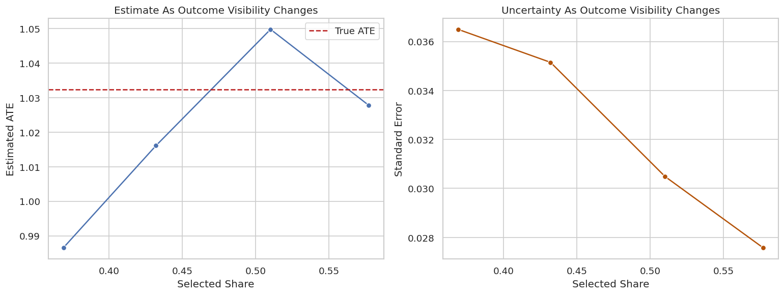
Selection Positivity Stress Test

This stress test shifts the selection equation so outcomes become easier or harder to observe. Lower selection rates usually increase uncertainty because fewer outcomes are available for the outcome regressions and inverse-selection correction.

stress_rows = []
for selection_shift in [-0.70, -0.35, 0.00, 0.35]:
    stress_probability = sigmoid(
        selection_shift
        - 0.25
        + 0.55 * mar_df["treated"]
        + 0.45 * mar_df["engagement_score"]
        - 0.55 * mar_df["support_need"]
        + 0.25 * mar_df["prior_usage"]
        + 0.70 * mar_df["selection_encouragement"]
    )
    stress_selected = rng.binomial(1, stress_probability)
    stress_df = mar_df.copy()
    stress_df["selected_stress"] = stress_selected
    stress_df["outcome_stress"] = stress_df["full_outcome"]
    stress_df.loc[stress_df["selected_stress"] == 0, "outcome_stress"] = 0.0

    stress_data = DoubleMLSSMData(
        stress_df,
        y_col="outcome_stress",
        d_cols="treated",
        s_col="selected_stress",
        x_cols=feature_cols_mar,
    )
    ml_g_stress, ml_pi_stress, ml_m_stress = make_linear_learners()
    stress_model = DoubleMLSSM(
        stress_data,
        ml_g=ml_g_stress,
        ml_pi=ml_pi_stress,
        ml_m=ml_m_stress,
        n_folds=5,
        score="missing-at-random",
    )
    stress_model.fit(store_predictions=False)
    stress_rows.append(
        {
            "selection_shift": selection_shift,
            "selected_share": stress_selected.mean(),
            "theta_hat": float(stress_model.coef[0]),
            "std_error": float(stress_model.se[0]),
            "true_target": TRUE_MAR_ATE,
            "bias_vs_target": float(stress_model.coef[0] - TRUE_MAR_ATE),
        }
    )

selection_stress = pd.DataFrame(stress_rows)
save_table(selection_stress, f"{NOTEBOOK_PREFIX}_selection_positivity_stress.csv")

fig, axes = plt.subplots(1, 2, figsize=(13, 5))
sns.lineplot(data=selection_stress, x="selected_share", y="theta_hat", marker="o", ax=axes[0])
axes[0].axhline(TRUE_MAR_ATE, color="#b91c1c", linestyle="--", label="True ATE")
axes[0].set_title("Estimate As Outcome Visibility Changes")
axes[0].set_xlabel("Selected Share")
axes[0].set_ylabel("Estimated ATE")
axes[0].legend()

sns.lineplot(data=selection_stress, x="selected_share", y="std_error", marker="o", color="#b45309", ax=axes[1])
axes[1].set_title("Uncertainty As Outcome Visibility Changes")
axes[1].set_xlabel("Selected Share")
axes[1].set_ylabel("Standard Error")

plt.tight_layout()
fig.savefig(FIGURE_DIR / f"{NOTEBOOK_PREFIX}_selection_positivity_stress.png", dpi=160, bbox_inches="tight")
plt.show()

display(selection_stress)

selection_shift selected_share theta_hat std_error true_target bias_vs_target
0 -0.70 0.368833 0.986534 0.036497 1.032326 -0.045792
1 -0.35 0.432000 1.016098 0.035148 1.032326 -0.016229
2 0.00 0.510167 1.049771 0.030484 1.032326 0.017444
3 0.35 0.577000 1.027837 0.027579 1.032326 -0.004490

The standard error tends to rise when fewer outcomes are observed. This is the practical cost of selected outcomes: even when the assumptions are correct, less outcome visibility means less information.

Nonignorable Selection Data

The next dataset adds a hidden response factor U. This hidden factor affects both outcome observation and the outcome itself. A missing-at-random analysis is now misspecified because conditioning on observed covariates is not enough.

We also add selection_encouragement, a variable that affects selection but does not directly affect the outcome. In the synthetic design, this variable satisfies the exclusion restriction. In real work, that restriction would require a domain argument.

rng_non = np.random.default_rng(RANDOM_SEED + 100)
N_NON = 6_000

non_engagement = rng_non.normal(0, 1, N_NON)
non_baseline = rng_non.normal(0, 1, N_NON)
non_support = rng_non.normal(0, 1, N_NON)
non_prior_usage = rng_non.normal(0, 1, N_NON)
non_mobile = rng_non.binomial(1, 0.48, N_NON)
non_selection_encouragement = rng_non.normal(0, 1, N_NON)
hidden_response_factor = rng_non.normal(0, 1, N_NON)

non_x = pd.DataFrame(
    {
        "engagement_score": non_engagement,
        "baseline_value": non_baseline,
        "support_need": non_support,
        "prior_usage": non_prior_usage,
        "mobile_user": non_mobile,
    }
)
feature_cols_non = list(non_x.columns)

non_treatment_propensity = sigmoid(-0.10 + 0.55 * non_engagement + 0.35 * non_baseline - 0.30 * non_support + 0.18 * non_mobile)
non_treated = rng_non.binomial(1, non_treatment_propensity)
non_tau = 1.00 + 0.25 * non_engagement + 0.15 * non_baseline - 0.10 * non_support + 0.08 * non_mobile
non_mu0 = 3.00 + 0.80 * non_engagement + 0.50 * non_baseline - 0.30 * non_support + 0.25 * non_prior_usage + 0.20 * non_mobile
non_full_outcome = non_mu0 + non_tau * non_treated + 0.60 * hidden_response_factor + rng_non.normal(0, 0.55, N_NON)

non_selection_probability = sigmoid(
    -0.25
    + 0.55 * non_treated
    + 0.45 * non_engagement
    - 0.55 * non_support
    + 0.25 * non_prior_usage
    + 0.85 * non_selection_encouragement
    + 0.75 * hidden_response_factor
)
non_selected = rng_non.binomial(1, non_selection_probability)
non_outcome_observed = non_full_outcome.copy()
non_outcome_observed[non_selected == 0] = 0.0

non_df = pd.concat(
    [
        pd.DataFrame({"row_id": np.arange(N_NON)}),
        non_x,
        pd.DataFrame(
            {
                "selection_encouragement": non_selection_encouragement,
                "treated": non_treated,
                "selected": non_selected,
                "outcome_observed": non_outcome_observed,
                "full_outcome": non_full_outcome,
                "true_tau": non_tau,
                "true_treatment_propensity": non_treatment_propensity,
                "true_selection_probability": non_selection_probability,
                "hidden_response_factor": hidden_response_factor,
            }
        ),
    ],
    axis=1,
)

TRUE_NON_ATE = non_df["true_tau"].mean()
non_path = DATASET_DIR / f"{NOTEBOOK_PREFIX}_synthetic_nonignorable_selection_data.csv"
non_df.to_csv(non_path, index=False)

print(f"Rows: {len(non_df):,}")
print(f"Selected share: {non_df['selected'].mean():.3f}")
print(f"True nonignorable-design ATE: {TRUE_NON_ATE:.4f}")
print(f"Saved data to: {non_path.relative_to(PROJECT_ROOT)}")
display(non_df.head())
Rows: 6,000
Selected share: 0.509
True nonignorable-design ATE: 1.0389
Saved data to: notebooks/tutorials/doubleml/outputs/datasets/08_synthetic_nonignorable_selection_data.csv
row_id engagement_score baseline_value support_need prior_usage mobile_user selection_encouragement treated selected outcome_observed full_outcome true_tau true_treatment_propensity true_selection_probability hidden_response_factor
0 0 -0.311445 -0.577787 -0.069680 0.874368 0 -1.616559 0 0 0.000000 1.737582 0.842439 0.388739 0.043021 -2.126387
1 1 -2.245198 0.178591 0.631997 -1.302306 1 -0.500702 0 0 0.000000 1.281574 0.482289 0.217218 0.075842 -0.188155
2 2 -0.214792 -0.104288 0.117372 -0.859742 0 0.019919 1 1 4.283298 4.283298 0.918922 0.428041 0.740645 1.478050
3 3 0.886864 0.208647 0.431936 -0.321071 1 -0.362617 1 1 5.454790 5.454790 1.289819 0.625093 0.550140 0.170938
4 4 0.174338 -0.218863 -0.605183 -0.134723 1 1.157343 1 0 0.000000 4.405956 1.151273 0.569752 0.851009 0.108234

This design deliberately violates missing-at-random selection. The hidden factor affects both selection and the outcome. The selection encouragement is available as an instrument-like variable for the nonignorable score.

Nonignorable Design Checks

Before fitting the nonignorable model, check that the selection encouragement is relevant for selection and not mechanically related to treatment. In synthetic data, we know it has no direct outcome effect, but applied work would need a real argument.

non_checks = pd.DataFrame(
    [
        {"metric": "selected_share", "value": non_df["selected"].mean()},
        {"metric": "treated_share", "value": non_df["treated"].mean()},
        {"metric": "corr_selection_encouragement_selected", "value": non_df["selection_encouragement"].corr(non_df["selected"])},
        {"metric": "corr_selection_encouragement_treated", "value": non_df["selection_encouragement"].corr(non_df["treated"])},
        {"metric": "corr_hidden_factor_selected", "value": non_df["hidden_response_factor"].corr(non_df["selected"])},
        {"metric": "corr_hidden_factor_full_outcome", "value": non_df["hidden_response_factor"].corr(non_df["full_outcome"])},
    ]
)
save_table(non_checks, f"{NOTEBOOK_PREFIX}_nonignorable_design_checks.csv")
display(non_checks)
metric value
0 selected_share 0.509000
1 treated_share 0.512667
2 corr_selection_encouragement_selected 0.300239
3 corr_selection_encouragement_treated 0.018788
4 corr_hidden_factor_selected 0.269843
5 corr_hidden_factor_full_outcome 0.372271

The selection encouragement is relevant for selection. The hidden factor is also related to selection and the outcome, which is why the missing-at-random analysis is no longer conceptually right.

MAR Versus Nonignorable Scores

Now we fit two models to the nonignorable dataset:

  • a missing-at-random score that treats the selection process as observed-covariate explainable;
  • a nonignorable score that uses selection_encouragement as a selection instrument.

The nonignorable backend passes selection_encouragement through z_cols instead of treating it as an ordinary covariate.

non_mar_features = feature_cols_non + ["selection_encouragement"]
non_mar_data = DoubleMLSSMData(
    non_df,
    y_col="outcome_observed",
    d_cols="treated",
    s_col="selected",
    x_cols=non_mar_features,
)
non_iv_data = DoubleMLSSMData(
    non_df,
    y_col="outcome_observed",
    d_cols="treated",
    s_col="selected",
    x_cols=feature_cols_non,
    z_cols="selection_encouragement",
)

non_rows = []

non_mar_g, non_mar_pi, non_mar_m = make_linear_learners()
wrong_mar_model = DoubleMLSSM(
    non_mar_data,
    ml_g=non_mar_g,
    ml_pi=non_mar_pi,
    ml_m=non_mar_m,
    n_folds=5,
    score="missing-at-random",
)
wrong_mar_model.fit(store_predictions=True)
non_rows.append(summarize_doubleml(wrong_mar_model, "MAR score on nonignorable data", "nonignorable data", TRUE_NON_ATE))

non_g, non_pi, non_m = make_linear_learners()
nonignorable_model = DoubleMLSSM(
    non_iv_data,
    ml_g=non_g,
    ml_pi=non_pi,
    ml_m=non_m,
    n_folds=5,
    score="nonignorable",
)
nonignorable_model.fit(store_predictions=True)
non_rows.append(summarize_doubleml(nonignorable_model, "Nonignorable score with selection instrument", "nonignorable data", TRUE_NON_ATE))

non_hgb_g, non_hgb_pi, non_hgb_m = make_hgb_learners(seed=RANDOM_SEED + 60, max_iter=70)
nonignorable_hgb = DoubleMLSSM(
    non_iv_data,
    ml_g=non_hgb_g,
    ml_pi=non_hgb_pi,
    ml_m=non_hgb_m,
    n_folds=5,
    score="nonignorable",
)
nonignorable_hgb.fit(store_predictions=True)
non_rows.append(summarize_doubleml(nonignorable_hgb, "Nonignorable score HGB", "nonignorable data", TRUE_NON_ATE))

nonignorable_summary = pd.DataFrame(non_rows)
save_table(nonignorable_summary, f"{NOTEBOOK_PREFIX}_nonignorable_score_comparison.csv")
display(nonignorable_summary)
estimator design theta_hat std_error ci_95_lower ci_95_upper true_target bias_vs_target
0 MAR score on nonignorable data nonignorable data 1.027318 0.035579 0.957586 1.097051 1.038926 -0.011607
1 Nonignorable score with selection instrument nonignorable data 1.070113 0.044343 0.983202 1.157024 1.038926 0.031187
2 Nonignorable score HGB nonignorable data 1.041098 0.046897 0.949182 1.133014 1.038926 0.002172

The nonignorable score uses extra structure to address a hidden selection path. The improvement is not automatic in every sample, and it depends on the selection encouragement being a credible exclusion variable.

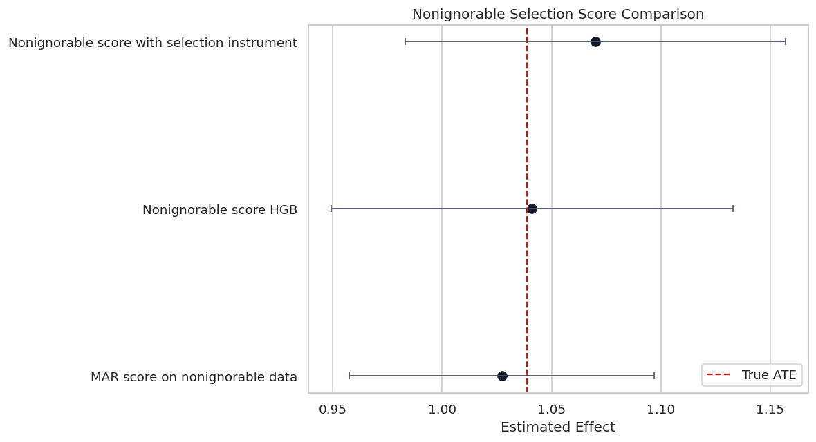
Nonignorable Estimate Plot

The plot below keeps the nonignorable comparison separate from the missing-at-random dataset because the data-generating process is different. The point is not to crown a universal best model; it is to show that the score must match the selection story.

plot_non = add_ci_columns(nonignorable_summary)
fig, ax = plt.subplots(figsize=(10, 5.5))
order = plot_non.sort_values("theta_hat", ascending=False)["estimator"]
sns.pointplot(
    data=plot_non,
    y="estimator",
    x="theta_hat",
    order=order,
    linestyle="none",
    color="#111827",
    errorbar=None,
    ax=ax,
)
for y_pos, (_, row) in enumerate(plot_non.set_index("estimator").loc[order].reset_index().iterrows()):
    ax.errorbar(
        x=row["theta_hat"],
        y=y_pos,
        xerr=[[row["lower_error"]], [row["upper_error"]]],
        fmt="none",
        color="#475569",
        capsize=3,
        linewidth=1.1,
    )
ax.axvline(TRUE_NON_ATE, color="#b91c1c", linestyle="--", linewidth=1.4, label="True ATE")
ax.set_title("Nonignorable Selection Score Comparison")
ax.set_xlabel("Estimated Effect")
ax.set_ylabel("")
ax.legend(loc="best")
plt.tight_layout()
fig.savefig(FIGURE_DIR / f"{NOTEBOOK_PREFIX}_nonignorable_estimate_comparison.png", dpi=160, bbox_inches="tight")
plt.show()

The figure makes the design choice visible. When hidden response behavior matters, a missing-at-random score is answering under the wrong assumption, even if it runs cleanly.

Combined Summary Table

This table collects the main estimates from the notebook. The rows should be compared within their design setting, not as interchangeable models.

combined_ssm_summary = pd.concat(
    [
        baseline_summary.assign(section="MAR data baselines"),
        manual_mar_summary.assign(section="MAR data manual score"),
        mar_doubleml_summary.assign(section="MAR data DoubleML"),
        nonignorable_summary.assign(section="nonignorable data"),
    ],
    ignore_index=True,
    sort=False,
)
save_table(combined_ssm_summary, f"{NOTEBOOK_PREFIX}_combined_ssm_summary.csv")
display(combined_ssm_summary)
estimator theta_hat std_error ci_95_lower ci_95_upper true_target bias_vs_target section design
0 Selected-row treated-control difference 1.675867 NaN NaN NaN 1.032326 0.643540 MAR data baselines NaN
1 Synthetic full-population treated-control diff... 1.732946 NaN NaN NaN 1.032326 0.700620 MAR data baselines NaN
2 Selected-row OLS with covariates 1.065852 0.026952 1.013027 1.118678 1.032326 0.033526 MAR data baselines NaN
3 Manual cross-fitted MAR SSM 1.003513 0.030544 0.943647 1.063380 1.032326 -0.028813 MAR data manual score NaN
4 MAR linear 1.001539 0.030564 0.941634 1.061444 1.032326 -0.030787 MAR data DoubleML missing-at-random
5 MAR HGB 1.002785 0.036305 0.931628 1.073943 1.032326 -0.029541 MAR data DoubleML missing-at-random
6 MAR HGB normalized IPW 1.023998 0.016952 0.990773 1.057222 1.032326 -0.008329 MAR data DoubleML missing-at-random
7 MAR score on nonignorable data 1.027318 0.035579 0.957586 1.097051 1.038926 -0.011607 nonignorable data nonignorable data
8 Nonignorable score with selection instrument 1.070113 0.044343 0.983202 1.157024 1.038926 0.031187 nonignorable data nonignorable data
9 Nonignorable score HGB 1.041098 0.046897 0.949182 1.133014 1.038926 0.002172 nonignorable data nonignorable data

The combined table shows the notebook’s main story: selected-row-only estimates can be very misleading, missing-at-random correction works when its assumptions match the data, and nonignorable selection requires stronger structure.

Reporting Checklist

A sample-selection report needs more than an effect estimate. The checklist below names the assumptions and diagnostics a reader should see.

ssm_reporting_checklist = pd.DataFrame(
    [
        {"topic": "target population", "question": "Is the effect for all rows or selected rows only?", "notebook_answer": "The main target is the full-population ATE."},
        {"topic": "selection definition", "question": "What does S=1 mean?", "notebook_answer": "The outcome is observed."},
        {"topic": "unselected rows", "question": "Were unselected rows retained?", "notebook_answer": "Yes. They enter treatment and selection nuisance models."},
        {"topic": "MAR assumption", "question": "Can observed D and X explain outcome observation?", "notebook_answer": "True in the MAR synthetic design, false in the nonignorable design."},
        {"topic": "selection overlap", "question": "Are selection probabilities away from zero?", "notebook_answer": "Checked with selection-probability histograms and stress tests."},
        {"topic": "treatment overlap", "question": "Are treatment propensities away from zero and one?", "notebook_answer": "Checked with treatment-propensity histograms."},
        {"topic": "nonignorable selection", "question": "If MAR is not credible, is there a valid selection instrument?", "notebook_answer": "The tutorial uses a synthetic selection encouragement as z_cols."},
        {"topic": "uncertainty", "question": "Are intervals and diagnostics reported?", "notebook_answer": "Yes. Standard errors, bootstrap CI, and nuisance diagnostics are saved."},
    ]
)
save_table(ssm_reporting_checklist, f"{NOTEBOOK_PREFIX}_ssm_reporting_checklist.csv")
display(ssm_reporting_checklist)
topic question notebook_answer
0 target population Is the effect for all rows or selected rows only? The main target is the full-population ATE.
1 selection definition What does S=1 mean? The outcome is observed.
2 unselected rows Were unselected rows retained? Yes. They enter treatment and selection nuisan...
3 MAR assumption Can observed D and X explain outcome observation? True in the MAR synthetic design, false in the...
4 selection overlap Are selection probabilities away from zero? Checked with selection-probability histograms ...
5 treatment overlap Are treatment propensities away from zero and ... Checked with treatment-propensity histograms.
6 nonignorable selection If MAR is not credible, is there a valid selec... The tutorial uses a synthetic selection encour...
7 uncertainty Are intervals and diagnostics reported? Yes. Standard errors, bootstrap CI, and nuisan...

This checklist turns the notebook into a reusable analysis template. The estimate is only one part of the evidence; the selection story is equally important.

Report Template

The final report template writes the preferred MAR result and the nonignorable comparison in plain language. The language is cautious because sample selection assumptions are often the hardest part of the design.

best_mar = mar_doubleml_summary.loc[mar_doubleml_summary["estimator"] == "MAR HGB"].iloc[0]
best_non = nonignorable_summary.loc[nonignorable_summary["estimator"] == "Nonignorable score with selection instrument"].iloc[0]

report_text = f"""
# Sample Selection DoubleML Report Template

## Question

Estimate the treatment effect for the full target population when the outcome is observed only for selected rows.

## Preferred Missing-At-Random Result

The preferred MAR estimate uses `DoubleMLSSM` with gradient boosting nuisance learners.

- Estimate: {best_mar['theta_hat']:.4f}
- Standard error: {best_mar['std_error']:.4f}
- 95 percent CI: [{best_mar['ci_95_lower']:.4f}, {best_mar['ci_95_upper']:.4f}]
- Synthetic true ATE: {TRUE_MAR_ATE:.4f}

## Nonignorable Selection Demonstration

When selection depends on a hidden response factor, a MAR score is not conceptually sufficient. The nonignorable score uses a selection encouragement variable as an exclusion variable.

- Nonignorable estimate: {best_non['theta_hat']:.4f}
- Standard error: {best_non['std_error']:.4f}
- 95 percent CI: [{best_non['ci_95_lower']:.4f}, {best_non['ci_95_upper']:.4f}]
- Synthetic true ATE: {TRUE_NON_ATE:.4f}

## Assumptions To State

- Treatment assignment is unconfounded after conditioning on observed covariates.
- Outcome observation is missing at random after conditioning on treatment and covariates, unless using the nonignorable score.
- Treatment and selection probabilities have adequate overlap.
- For nonignorable selection, the selection encouragement affects outcome observation and has no direct outcome effect.

## Diagnostics To Include

- Selected versus unselected covariate balance.
- Treatment and selection probability overlap.
- Selected-row baseline estimates versus selection-adjusted estimates.
- Nuisance learner diagnostics.
- Stress test showing how lower outcome visibility affects uncertainty.
""".strip()

report_path = REPORT_DIR / f"{NOTEBOOK_PREFIX}_ssm_report_template.md"
report_path.write_text(report_text)
print(report_text)
# Sample Selection DoubleML Report Template

## Question

Estimate the treatment effect for the full target population when the outcome is observed only for selected rows.

## Preferred Missing-At-Random Result

The preferred MAR estimate uses `DoubleMLSSM` with gradient boosting nuisance learners.

- Estimate: 1.0028
- Standard error: 0.0363
- 95 percent CI: [0.9316, 1.0739]
- Synthetic true ATE: 1.0323

## Nonignorable Selection Demonstration

When selection depends on a hidden response factor, a MAR score is not conceptually sufficient. The nonignorable score uses a selection encouragement variable as an exclusion variable.

- Nonignorable estimate: 1.0701
- Standard error: 0.0443
- 95 percent CI: [0.9832, 1.1570]
- Synthetic true ATE: 1.0389

## Assumptions To State

- Treatment assignment is unconfounded after conditioning on observed covariates.
- Outcome observation is missing at random after conditioning on treatment and covariates, unless using the nonignorable score.
- Treatment and selection probabilities have adequate overlap.
- For nonignorable selection, the selection encouragement affects outcome observation and has no direct outcome effect.

## Diagnostics To Include

- Selected versus unselected covariate balance.
- Treatment and selection probability overlap.
- Selected-row baseline estimates versus selection-adjusted estimates.
- Nuisance learner diagnostics.
- Stress test showing how lower outcome visibility affects uncertainty.

The report template keeps the estimate tied to its assumptions. That is especially important for selected-outcome data, where the missing outcomes are precisely the part we cannot inspect directly.

Artifact Manifest

The manifest lists every dataset, figure, table, and report produced by this notebook. This makes the tutorial easy to audit and reuse.

artifact_rows = []
for folder, artifact_type in [
    (DATASET_DIR, "dataset"),
    (TABLE_DIR, "table"),
    (FIGURE_DIR, "figure"),
    (REPORT_DIR, "report"),
]:
    for file_path in sorted(folder.glob(f"{NOTEBOOK_PREFIX}_*")):
        artifact_rows.append(
            {
                "artifact_type": artifact_type,
                "file_name": file_path.name,
                "relative_path": str(file_path.relative_to(PROJECT_ROOT)),
            }
        )

artifact_manifest = pd.DataFrame(artifact_rows)
save_table(artifact_manifest, f"{NOTEBOOK_PREFIX}_artifact_manifest.csv")
display(artifact_manifest)
artifact_type file_name relative_path
0 dataset 08_synthetic_mar_selection_data.csv notebooks/tutorials/doubleml/outputs/datasets/...
1 dataset 08_synthetic_nonignorable_selection_data.csv notebooks/tutorials/doubleml/outputs/datasets/...
2 table 08_artifact_manifest.csv notebooks/tutorials/doubleml/outputs/tables/08...
3 table 08_combined_ssm_summary.csv notebooks/tutorials/doubleml/outputs/tables/08...
4 table 08_manual_mar_ssm_diagnostics.csv notebooks/tutorials/doubleml/outputs/tables/08...
5 table 08_manual_mar_ssm_summary.csv notebooks/tutorials/doubleml/outputs/tables/08...
6 table 08_mar_baseline_estimates.csv notebooks/tutorials/doubleml/outputs/tables/08...
7 table 08_mar_data_audit.csv notebooks/tutorials/doubleml/outputs/tables/08...
8 table 08_mar_doublemlssm_backend.csv notebooks/tutorials/doubleml/outputs/tables/08...
9 table 08_mar_doublemlssm_summary.csv notebooks/tutorials/doubleml/outputs/tables/08...
10 table 08_mar_estimate_comparison.csv notebooks/tutorials/doubleml/outputs/tables/08...
11 table 08_mar_field_dictionary.csv notebooks/tutorials/doubleml/outputs/tables/08...
12 table 08_mar_hgb_bootstrap_ci.csv notebooks/tutorials/doubleml/outputs/tables/08...
13 table 08_mar_hgb_prediction_quality.csv notebooks/tutorials/doubleml/outputs/tables/08...
14 table 08_mar_nuisance_losses.csv notebooks/tutorials/doubleml/outputs/tables/08...
15 table 08_mar_selection_covariate_balance.csv notebooks/tutorials/doubleml/outputs/tables/08...
16 table 08_mar_treatment_selection_cells.csv notebooks/tutorials/doubleml/outputs/tables/08...
17 table 08_nonignorable_design_checks.csv notebooks/tutorials/doubleml/outputs/tables/08...
18 table 08_nonignorable_score_comparison.csv notebooks/tutorials/doubleml/outputs/tables/08...
19 table 08_package_versions.csv notebooks/tutorials/doubleml/outputs/tables/08...
20 table 08_selection_positivity_stress.csv notebooks/tutorials/doubleml/outputs/tables/08...
21 table 08_ssm_reporting_checklist.csv notebooks/tutorials/doubleml/outputs/tables/08...
22 figure 08_manual_mar_score_diagnostics.png notebooks/tutorials/doubleml/outputs/figures/0...
23 figure 08_mar_estimate_comparison.png notebooks/tutorials/doubleml/outputs/figures/0...
24 figure 08_mar_overlap_diagnostics.png notebooks/tutorials/doubleml/outputs/figures/0...
25 figure 08_mar_selection_and_outcome_visibility.png notebooks/tutorials/doubleml/outputs/figures/0...
26 figure 08_nonignorable_estimate_comparison.png notebooks/tutorials/doubleml/outputs/figures/0...
27 figure 08_selection_positivity_stress.png notebooks/tutorials/doubleml/outputs/figures/0...
28 figure 08_ssm_design_dag.png notebooks/tutorials/doubleml/outputs/figures/0...
29 report 08_ssm_report_template.md notebooks/tutorials/doubleml/outputs/reports/0...

The sample-selection notebook is complete. The next natural topic is regression discontinuity design, where identification comes from continuity around a cutoff rather than selection correction, instruments, or parallel trends.