DoubleML Tutorial 06: Interactive IV Model IIVM

This notebook is a full tutorial on DoubleMLIIVM, the interactive instrumental-variable model for a binary treatment and a binary instrument.

The previous notebook handled binary treatments under observed-control adjustment. Here we add noncompliance and instrument-induced treatment changes. The treatment is binary, the instrument is binary, and the target is a local effect: the effect for units whose treatment status is shifted by the instrument.

The main point is conceptual as much as computational. Binary IV estimates are not ordinary ATE estimates. They are local effects tied to compliance behavior and instrument validity.

Learning Goals

By the end of this notebook, you should be able to:

• Explain the IIVM setup for binary treatment and binary instrument data.
• Distinguish ATE, ATT-style targets, and LATE.
• Explain compliers, always-takers, never-takers, and defiers.
• State the IV assumptions for binary instruments: relevance, exclusion, independence after controls, and monotonicity.
• Understand the DoubleMLIIVM nuisance roles: ml_g, ml_m, and ml_r.
• Manually compute the cross-fitted IIVM ratio score.
• Fit DoubleMLIIVM and diagnose first-stage strength, instrument overlap, nuisance losses, score contributions, and split stability.
• Explain why weak instruments, invalid instruments, or wrong subgroup assumptions change the meaning of the estimate.

From ATE To LATE

For a binary treatment, the ATE is:

\[ E[Y(1)-Y(0)]. \]

That target averages treatment effects over everyone. In a binary IV design with noncompliance, the instrument does not necessarily move everyone into treatment. Some units take treatment regardless of the instrument, some never take treatment, and some take treatment only when encouraged.

The local average treatment effect is the treatment effect for the instrument-responsive units:

\[ LATE = E[Y(1)-Y(0) \mid \text{complier}]. \]

When compliance probability varies with covariates, the model target is a compliance-weighted local effect. In the synthetic data we can compute that target exactly; in real data we usually cannot observe compliance type directly.

Compliance Types

With a binary instrument Z and binary treatment D, define two potential treatment states:

\[ D(1) \quad \text{and} \quad D(0). \]

D(1) is whether the unit would take treatment if instrumented. D(0) is whether the unit would take treatment if not instrumented.

The common compliance types are:

• Complier: D(1)=1, D(0)=0.
• Always-taker: D(1)=1, D(0)=1.
• Never-taker: D(1)=0, D(0)=0.
• Defier: D(1)=0, D(0)=1.

The usual monotonicity assumption rules out defiers: the instrument should not make anyone less likely to take treatment.

IIVM Assumptions

A binary IV design needs several assumptions:

• Relevance: the instrument changes treatment probability after adjusting for controls.
• Exclusion: the instrument affects the outcome only through treatment.
• Conditional independence: after adjusting for controls, the instrument is independent of potential outcomes and potential treatment states.
• Monotonicity: the instrument does not push some units in the opposite direction.
• Overlap for the instrument: every relevant covariate profile has a nonzero chance of both instrument states.

The data can help screen relevance and overlap. Exclusion, independence, and monotonicity require design evidence.

IIVM Nuisance Functions

DoubleMLIIVM estimates these nuisance components:

\[ g_0(0, X) = E[Y \mid Z=0, X] \]

\[ g_0(1, X) = E[Y \mid Z=1, X] \]

\[ m_0(X) = P(Z=1 \mid X) \]

and

\[ r_0(0, X) = P(D=1 \mid Z=0, X), \quad r_0(1, X) = P(D=1 \mid Z=1, X). \]

In the API:

• ml_g predicts the outcome as a function of instrument status and controls.
• ml_m predicts the instrument propensity.
• ml_r predicts treatment take-up as a function of instrument status and controls.

The target is the ratio:

\[ \theta_0 = \frac{E[g_0(1,X)-g_0(0,X)]}{E[r_0(1,X)-r_0(0,X)]}. \]

Runtime Note

This notebook fits several cross-fitted binary IV models, a manual IIVM estimator, subgroup comparisons, and a repeated-splitting check. On a typical laptop, the full run should take roughly two to five minutes.

The stress tests use synthetic oracle calculations where possible so that the conceptual lessons stay fast.

Setup

This cell prepares the notebook environment. It creates output folders, keeps matplotlib cache files inside the tutorial output folder, imports scientific Python libraries, and records package versions.

The path logic supports running from the repository root or directly from the tutorial folder.

from pathlib import Path
import os
import warnings

NOTEBOOK_PREFIX = "06"
RANDOM_STATE = 2026

CURRENT_DIR = Path.cwd().resolve()
if CURRENT_DIR.name == "doubleml":
    REPO_ROOT = CURRENT_DIR.parents[2]
elif (CURRENT_DIR / "notebooks" / "tutorials" / "doubleml").exists():
    REPO_ROOT = CURRENT_DIR
else:
    REPO_ROOT = CURRENT_DIR

OUTPUT_DIR = REPO_ROOT / "notebooks" / "tutorials" / "doubleml" / "outputs"
DATASET_DIR = OUTPUT_DIR / "datasets"
FIGURE_DIR = OUTPUT_DIR / "figures"
TABLE_DIR = OUTPUT_DIR / "tables"
REPORT_DIR = OUTPUT_DIR / "reports"
MATPLOTLIB_CACHE_DIR = OUTPUT_DIR / "matplotlib_cache"

for directory in [DATASET_DIR, FIGURE_DIR, TABLE_DIR, REPORT_DIR, MATPLOTLIB_CACHE_DIR]:
    directory.mkdir(parents=True, exist_ok=True)

os.environ.setdefault("MPLCONFIGDIR", str(MATPLOTLIB_CACHE_DIR))
warnings.filterwarnings("ignore", category=FutureWarning)
warnings.filterwarnings("ignore", category=DeprecationWarning)
warnings.filterwarnings("ignore", message="IProgress not found.*")
warnings.filterwarnings("ignore", message=".*X does not have valid feature names.*")

import numpy as np
import pandas as pd
import matplotlib.pyplot as plt
import seaborn as sns
from IPython.display import display

from sklearn.base import clone
from sklearn.ensemble import HistGradientBoostingClassifier, HistGradientBoostingRegressor
from sklearn.exceptions import ConvergenceWarning
from sklearn.linear_model import LassoCV, LinearRegression, LogisticRegressionCV
from sklearn.metrics import log_loss, mean_absolute_error, mean_squared_error, roc_auc_score, r2_score
from sklearn.model_selection import KFold
from sklearn.pipeline import make_pipeline
from sklearn.preprocessing import StandardScaler

import statsmodels.api as sm

import doubleml as dml
from doubleml import DoubleMLData, DoubleMLIIVM, DoubleMLIRM

warnings.filterwarnings("ignore", category=ConvergenceWarning)

sns.set_theme(style="whitegrid", context="notebook")
plt.rcParams["figure.figsize"] = (10, 5)
plt.rcParams["axes.titleweight"] = "bold"

package_versions = pd.DataFrame(
    [
        {"package": "doubleml", "version": dml.__version__},
        {"package": "numpy", "version": np.__version__},
        {"package": "pandas", "version": pd.__version__},
        {"package": "seaborn", "version": sns.__version__},
        {"package": "statsmodels", "version": sm.__version__},
    ]
)
package_versions.to_csv(TABLE_DIR / f"{NOTEBOOK_PREFIX}_package_versions.csv", index=False)
display(package_versions)

	package	version
0	doubleml	0.11.2
1	numpy	2.4.4
2	pandas	3.0.2
3	seaborn	0.13.2
4	statsmodels	0.14.6

The package table is saved as part of the reproducibility record. Binary IV workflows depend on classifier behavior, cross-fitting splits, and package defaults.

Helper Functions

The next cell defines utilities for saving tables, computing simple baselines, computing manual ratio scores, cross-fitting IIVM nuisance functions, and extracting DoubleML diagnostics.

The manual IIVM formula is the most important helper. It estimates a numerator effect of the instrument on the outcome and a denominator effect of the instrument on treatment, then takes their ratio.

def save_table(df, name):
    path = TABLE_DIR / f"{NOTEBOOK_PREFIX}_{name}.csv"
    df.to_csv(path, index=False)
    return df


def sigmoid(x):
    return 1.0 / (1.0 + np.exp(-x))


def rmse(y_true, y_pred):
    return float(np.sqrt(mean_squared_error(y_true, y_pred)))


def mean_difference_summary(y, group, label, target="difference"):
    group = np.asarray(group)
    y = np.asarray(y)
    high = y[group == 1]
    low = y[group == 0]
    theta_hat = float(high.mean() - low.mean())
    std_error = float(np.sqrt(high.var(ddof=1) / len(high) + low.var(ddof=1) / len(low)))
    return {
        "estimator": label,
        "target": target,
        "theta_hat": theta_hat,
        "std_error": std_error,
        "ci_95_lower": theta_hat - 1.96 * std_error,
        "ci_95_upper": theta_hat + 1.96 * std_error,
        "p_value": np.nan,
    }


def treatment_ols_summary(y, X, treatment_col, label):
    X_design = sm.add_constant(X, has_constant="add")
    fit = sm.OLS(y, X_design).fit(cov_type="HC1")
    row = fit.summary2().tables[1].loc[treatment_col]
    return {
        "estimator": label,
        "target": "observed-control treatment slope",
        "theta_hat": float(row["Coef."]),
        "std_error": float(row["Std.Err."]),
        "ci_95_lower": float(row["[0.025"]),
        "ci_95_upper": float(row["0.975]"]),
        "p_value": float(row["P>|z|"]),
    }


def wald_summary(y, d, z, label):
    y = np.asarray(y)
    d = np.asarray(d)
    z = np.asarray(z)
    numerator = y[z == 1].mean() - y[z == 0].mean()
    denominator = d[z == 1].mean() - d[z == 0].mean()
    theta_hat = float(numerator / denominator)
    influence = (z / z.mean()) * (y - theta_hat * d) - ((1 - z) / (1 - z).mean()) * (y - theta_hat * d)
    std_error = float(np.std(influence, ddof=1) / (abs(denominator) * np.sqrt(len(y))))
    return {
        "estimator": label,
        "target": "raw Wald LATE-style ratio",
        "theta_hat": theta_hat,
        "std_error": std_error,
        "ci_95_lower": theta_hat - 1.96 * std_error,
        "ci_95_upper": theta_hat + 1.96 * std_error,
        "p_value": np.nan,
        "wald_numerator": float(numerator),
        "wald_denominator": float(denominator),
    }


def residualized_wald_summary(y, d, z, X, label):
    y_resid = y - LinearRegression().fit(X, y).predict(X)
    d_resid = d - LinearRegression().fit(X, d).predict(X)
    z_resid = z - LinearRegression().fit(X, z).predict(X)
    numerator = float(np.mean(z_resid * y_resid))
    denominator = float(np.mean(z_resid * d_resid))
    theta_hat = numerator / denominator
    psi = z_resid * (y_resid - theta_hat * d_resid)
    std_error = float(np.sqrt(np.mean(psi ** 2) / (denominator ** 2 * len(y))))
    return {
        "estimator": label,
        "target": "linear residualized Wald ratio",
        "theta_hat": float(theta_hat),
        "std_error": std_error,
        "ci_95_lower": theta_hat - 1.96 * std_error,
        "ci_95_upper": theta_hat + 1.96 * std_error,
        "p_value": np.nan,
        "wald_numerator": numerator,
        "wald_denominator": denominator,
    }


def iivm_ratio_summary(y, d, z, g0_hat, g1_hat, m_hat, r0_hat, r1_hat, label):
    y = np.asarray(y)
    d = np.asarray(d)
    z = np.asarray(z)
    m_hat = np.clip(np.asarray(m_hat), 0.02, 0.98)
    g0_hat = np.asarray(g0_hat)
    g1_hat = np.asarray(g1_hat)
    r0_hat = np.clip(np.asarray(r0_hat), 0.01, 0.99)
    r1_hat = np.clip(np.asarray(r1_hat), 0.01, 0.99)

    numerator_score = g1_hat - g0_hat + z * (y - g1_hat) / m_hat - (1 - z) * (y - g0_hat) / (1 - m_hat)
    denominator_score = r1_hat - r0_hat + z * (d - r1_hat) / m_hat - (1 - z) * (d - r0_hat) / (1 - m_hat)
    numerator = float(np.mean(numerator_score))
    denominator = float(np.mean(denominator_score))
    theta_hat = numerator / denominator
    ratio_score = numerator_score - theta_hat * denominator_score
    std_error = float(np.std(ratio_score, ddof=1) / (abs(denominator) * np.sqrt(len(y))))
    return {
        "estimator": label,
        "target": "LATE",
        "theta_hat": float(theta_hat),
        "std_error": std_error,
        "ci_95_lower": theta_hat - 1.96 * std_error,
        "ci_95_upper": theta_hat + 1.96 * std_error,
        "p_value": np.nan,
        "iivm_numerator": numerator,
        "iivm_denominator": denominator,
    }


def crossfit_iivm_nuisances(X, y, d, z, outcome_learner, instrument_learner, treatment_learner, n_splits=5, random_state=RANDOM_STATE):
    cv = KFold(n_splits=n_splits, shuffle=True, random_state=random_state)
    g0_hat = np.zeros(len(y))
    g1_hat = np.zeros(len(y))
    m_hat = np.zeros(len(y))
    r0_hat = np.zeros(len(y))
    r1_hat = np.zeros(len(y))

    for train_idx, test_idx in cv.split(X):
        X_train = X.iloc[train_idx]
        X_test = X.iloc[test_idx]
        y_train = y[train_idx]
        d_train = d[train_idx]
        z_train = z[train_idx]

        g0_model = clone(outcome_learner).fit(X_train[z_train == 0], y_train[z_train == 0])
        g1_model = clone(outcome_learner).fit(X_train[z_train == 1], y_train[z_train == 1])
        m_model = clone(instrument_learner).fit(X_train, z_train)
        r0_model = clone(treatment_learner).fit(X_train[z_train == 0], d_train[z_train == 0])
        r1_model = clone(treatment_learner).fit(X_train[z_train == 1], d_train[z_train == 1])

        g0_hat[test_idx] = g0_model.predict(X_test)
        g1_hat[test_idx] = g1_model.predict(X_test)
        m_hat[test_idx] = m_model.predict_proba(X_test)[:, 1]
        r0_hat[test_idx] = r0_model.predict_proba(X_test)[:, 1]
        r1_hat[test_idx] = r1_model.predict_proba(X_test)[:, 1]

    return g0_hat, g1_hat, np.clip(m_hat, 0.02, 0.98), np.clip(r0_hat, 0.01, 0.99), np.clip(r1_hat, 0.01, 0.99)


def prediction_vector(doubleml_model, learner_key):
    arr = np.asarray(doubleml_model.predictions[learner_key])
    if arr.ndim != 3:
        raise ValueError(f"Expected a 3D prediction array, got shape {arr.shape}")
    return arr[:, 0, 0]


def learner_loss_table(doubleml_model, model_label):
    losses = doubleml_model.evaluate_learners()
    rows = []
    for learner_name, values in losses.items():
        arr = np.asarray(values)
        rows.append(
            {
                "model": model_label,
                "learner": learner_name,
                "mean_loss": float(np.mean(arr)),
                "min_loss": float(np.min(arr)),
                "max_loss": float(np.max(arr)),
            }
        )
    return pd.DataFrame(rows)

The manual ratio helper mirrors the IIVM target: an instrument-outcome effect divided by an instrument-treatment effect. The denominator is the first stage. If that denominator is small, the estimate becomes unstable.

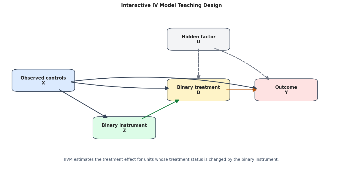
Draw The Binary IV Design

The diagram below shows the core binary IV story.

The instrument Z shifts treatment D. Treatment affects outcome Y. Observed controls X may affect all three. Hidden factors can affect treatment and outcome, which is why observed-control IRM may fail. The IV design requires that the hidden factors do not also drive the instrument after conditioning on X, and that the instrument has no direct outcome path.

from matplotlib.patches import FancyBboxPatch, FancyArrowPatch

nodes = {
    "X": {"xy": (0.12, 0.58), "label": "Observed controls\nX", "color": "#dbeafe"},
    "Z": {"xy": (0.36, 0.28), "label": "Binary instrument\nZ", "color": "#dcfce7"},
    "D": {"xy": (0.58, 0.52), "label": "Binary treatment\nD", "color": "#fef3c7"},
    "Y": {"xy": (0.84, 0.52), "label": "Outcome\nY", "color": "#fee2e2"},
    "U": {"xy": (0.58, 0.84), "label": "Hidden factor\nU", "color": "#f3f4f6"},
}

edge_specs = [
    ("X", "Z", "#334155", "solid", 0.00),
    ("X", "D", "#334155", "solid", 0.04),
    ("X", "Y", "#334155", "solid", -0.08),
    ("Z", "D", "#15803d", "solid", 0.00),
    ("D", "Y", "#b45309", "solid", 0.00),
    ("U", "D", "#6b7280", "dashed", 0.00),
    ("U", "Y", "#6b7280", "dashed", -0.10),
]

fig, ax = plt.subplots(figsize=(12, 6.2))
ax.set_axis_off()
box_w, box_h = 0.15, 0.105

def edge_endpoint(source_xy, target_xy, from_source=True):
    x0, y0 = source_xy
    x1, y1 = target_xy
    dx, dy = x1 - x0, y1 - y0
    scale = 1.0 / max(abs(dx) / (box_w / 2), abs(dy) / (box_h / 2))
    if from_source:
        return (x0 + dx * scale * 1.08, y0 + dy * scale * 1.08)
    return (x1 - dx * scale * 1.12, y1 - dy * scale * 1.12)

for spec in nodes.values():
    x, y_pos = spec["xy"]
    rect = FancyBboxPatch(
        (x - box_w / 2, y_pos - box_h / 2),
        box_w,
        box_h,
        boxstyle="round,pad=0.018",
        facecolor=spec["color"],
        edgecolor="#334155",
        linewidth=1.2,
        zorder=3,
    )
    ax.add_patch(rect)
    ax.text(x, y_pos, spec["label"], ha="center", va="center", fontsize=11, fontweight="bold", zorder=4)

for start, end, color, style, rad in edge_specs:
    start_xy = edge_endpoint(nodes[start]["xy"], nodes[end]["xy"], from_source=True)
    end_xy = edge_endpoint(nodes[start]["xy"], nodes[end]["xy"], from_source=False)
    arrow = FancyArrowPatch(
        start_xy,
        end_xy,
        arrowstyle="-|>",
        mutation_scale=20,
        linewidth=1.8,
        color=color,
        linestyle=style,
        connectionstyle=f"arc3,rad={rad}",
        zorder=5,
    )
    ax.add_patch(arrow)

ax.text(
    0.50,
    0.08,
    "IIVM estimates the treatment effect for units whose treatment status is changed by the binary instrument.",
    ha="center",
    va="center",
    fontsize=10,
    color="#475569",
)
ax.set_title("Interactive IV Model Teaching Design", pad=18)
plt.tight_layout()
fig.savefig(FIGURE_DIR / f"{NOTEBOOK_PREFIX}_iivm_design_dag.png", dpi=160, bbox_inches="tight")
plt.show()

The diagram makes clear why this is not the same as the IRM notebook. The instrument creates a local source of treatment variation, and the estimate is tied to that variation.

Create A Teaching Dataset With Noncompliance

We now simulate a binary instrument and a binary treatment.

The instrument is an encouragement. Some units always take treatment, some never take treatment, and some comply with the encouragement. There are no defiers, so monotonicity holds by construction.

The outcome depends on the actual treatment, observed controls, and a latent factor related to compliance type. This makes direct treatment comparisons biased, but the instrument remains valid after conditioning on observed controls.

rng = np.random.default_rng(RANDOM_STATE)
N_OBS = 5_000

feature_cols = [
    "engagement_score",
    "need_intensity",
    "content_fit",
    "recent_activity",
    "price_sensitivity",
    "tenure_signal",
    "novelty_appetite",
    "seasonality_signal",
]

X_raw = pd.DataFrame(rng.normal(size=(N_OBS, len(feature_cols))), columns=feature_cols)

true_instrument_logit = (
    -0.10
    + 0.55 * X_raw["engagement_score"]
    - 0.35 * X_raw["price_sensitivity"]
    + 0.25 * np.sin(X_raw["content_fit"])
    + 0.20 * X_raw["seasonality_signal"]
)
true_instrument_propensity = np.clip(sigmoid(true_instrument_logit), 0.08, 0.92)
encouragement = rng.binomial(1, true_instrument_propensity, size=N_OBS)

p_complier = (
    0.45
    + 0.15 * np.tanh(X_raw["need_intensity"])
    + 0.10 * np.tanh(X_raw["novelty_appetite"])
    - 0.08 * np.tanh(X_raw["price_sensitivity"])
)
p_always = 0.18 + 0.07 * np.tanh(X_raw["engagement_score"])
p_complier = np.clip(p_complier, 0.15, 0.70)
p_always = np.clip(p_always, 0.05, 0.35)
p_never = np.clip(1 - p_complier - p_always, 0.05, 0.80)
prob_sum = p_complier + p_always + p_never
p_complier = p_complier / prob_sum
p_always = p_always / prob_sum
p_never = p_never / prob_sum

compliance_draw = rng.uniform(size=N_OBS)
compliance_type = np.where(
    compliance_draw < p_always,
    "always_taker",
    np.where(compliance_draw < p_always + p_complier, "complier", "never_taker"),
)

feature_exposure = np.where(
    compliance_type == "always_taker",
    1,
    np.where(compliance_type == "never_taker", 0, encouragement),
)

latent_compliance_factor = (
    np.where(compliance_type == "always_taker", 0.50, np.where(compliance_type == "never_taker", -0.20, 0.00))
    + rng.normal(loc=0.0, scale=0.40, size=N_OBS)
)

true_mu0 = (
    0.70 * np.sin(X_raw["engagement_score"])
    + 0.45 * X_raw["need_intensity"] ** 2
    - 0.35 * X_raw["price_sensitivity"]
    + 0.25 * X_raw["content_fit"] * X_raw["recent_activity"]
    + 0.35 * latent_compliance_factor
)
true_tau = (
    0.80
    + 0.25 * sigmoid(X_raw["engagement_score"])
    + 0.25 * X_raw["need_intensity"]
    - 0.15 * X_raw["price_sensitivity"]
    + 0.20 * (X_raw["novelty_appetite"] > 0).astype(float)
)
true_mu1 = true_mu0 + true_tau
outcome_noise = rng.normal(loc=0.0, scale=1.0, size=N_OBS)
weekly_value = true_mu0 + true_tau * feature_exposure + outcome_noise

# Population-level IIVM targets under the synthetic design.
TRUE_ATE = float(np.mean(true_tau))
TRUE_REALIZED_COMPLIER_EFFECT = float(np.mean(true_tau[compliance_type == "complier"]))
TRUE_LATE = float(np.mean(p_complier * true_tau) / np.mean(p_complier))
TRUE_FIRST_STAGE = float(np.mean(p_complier))

# Oracle conditional mean functions for the IIVM ratio.
true_r0 = p_always
true_r1 = p_always + p_complier
true_g0 = true_mu0 + true_tau * true_r0
true_g1 = true_mu0 + true_tau * true_r1

# Potential treatment states are useful for teaching compliance types.
potential_d0 = np.where(compliance_type == "always_taker", 1, 0)
potential_d1 = np.where(compliance_type == "never_taker", 0, 1)

iivm_df = X_raw.assign(
    encouragement=encouragement,
    feature_exposure=feature_exposure,
    weekly_value=weekly_value,
    compliance_type=compliance_type,
    true_instrument_propensity=true_instrument_propensity,
    true_p_complier=p_complier,
    true_p_always=p_always,
    true_p_never=p_never,
    true_r0=true_r0,
    true_r1=true_r1,
    true_g0=true_g0,
    true_g1=true_g1,
    true_mu0=true_mu0,
    true_mu1=true_mu1,
    true_tau=true_tau,
    latent_compliance_factor=latent_compliance_factor,
    potential_d0=potential_d0,
    potential_d1=potential_d1,
)

iivm_df.to_csv(DATASET_DIR / f"{NOTEBOOK_PREFIX}_synthetic_iivm_data.csv", index=False)
print(f"Saved synthetic IIVM data with shape {iivm_df.shape}")
print(f"Instrument rate: {iivm_df['encouragement'].mean():.3f}")
print(f"Treatment rate: {iivm_df['feature_exposure'].mean():.3f}")
print(f"True ATE: {TRUE_ATE:.3f}")
print(f"True compliance-weighted LATE: {TRUE_LATE:.3f}")
print(f"True realized complier effect: {TRUE_REALIZED_COMPLIER_EFFECT:.3f}")
print(f"True first stage: {TRUE_FIRST_STAGE:.3f}")
display(iivm_df.head())

Saved synthetic IIVM data with shape (5000, 26)
Instrument rate: 0.463
Treatment rate: 0.392
True ATE: 1.021
True compliance-weighted LATE: 1.102
True realized complier effect: 1.098
True first stage: 0.448

	engagement_score	need_intensity	content_fit	recent_activity	price_sensitivity	tenure_signal	novelty_appetite	seasonality_signal	encouragement	feature_exposure	...	true_r0	true_r1	true_g0	true_g1	true_mu0	true_mu1	true_tau	latent_compliance_factor	potential_d0	potential_d1
0	-0.793122	0.240571	-1.896326	1.395772	0.638295	-0.292047	-0.311949	0.303835	0	0	...	0.133788	0.543873	-1.272362	-0.926958	-1.385047	-0.542774	0.842273	-0.077700	0	1
1	-0.267660	-0.225909	0.720068	0.514705	-0.064128	-0.085477	0.160916	-0.614018	0	0	...	0.161699	0.599455	0.076353	0.541036	-0.095292	0.966220	1.061512	-0.137787	0	0
2	-0.403750	0.548260	-0.130483	-1.374426	-0.477279	0.656622	-0.232283	-0.148733	0	0	...	0.153179	0.690767	0.238566	0.834622	0.068727	1.177487	1.108760	-0.009748	0	0
3	0.641837	1.824610	-0.713189	1.348207	-1.230013	0.174978	-1.169530	1.351458	0	0	...	0.219630	0.797019	2.368826	3.295216	2.016441	3.620887	1.604447	-0.259689	0	1
4	0.833923	1.137717	-0.885533	0.684555	-0.519013	-0.457385	0.506537	0.876718	1	1	...	0.227780	0.884706	1.558963	2.568380	1.208961	2.745538	1.536577	0.222783	0	1

5 rows × 26 columns

The true ATE and true local effect differ because the instrument-responsive units have a different treatment-effect mix than the full population. That is the key conceptual difference between IRM and IIVM.

Field Dictionary

This table documents the roles of the important columns. The hidden teaching columns are not available in real applications; they are present only so the tutorial can compare estimates with known synthetic truth.

field_dictionary = pd.DataFrame(
    [
        {"column": "weekly_value", "role": "outcome", "description": "Observed outcome Y."},
        {"column": "feature_exposure", "role": "binary treatment", "description": "Observed binary treatment D."},
        {"column": "encouragement", "role": "binary instrument", "description": "Observed binary instrument Z."},
        *[
            {"column": col, "role": "control", "description": "Observed pre-treatment control X."}
            for col in feature_cols
        ],
        {"column": "compliance_type", "role": "hidden teaching column", "description": "Realized synthetic compliance type; not observed in ordinary IV data."},
        {"column": "true_instrument_propensity", "role": "hidden teaching column", "description": "True P(Z=1 | X)."},
        {"column": "true_p_complier", "role": "hidden teaching column", "description": "True conditional probability of complier type."},
        {"column": "true_p_always", "role": "hidden teaching column", "description": "True conditional probability of always-taker type."},
        {"column": "true_p_never", "role": "hidden teaching column", "description": "True conditional probability of never-taker type."},
        {"column": "true_r0", "role": "hidden teaching column", "description": "True P(D=1 | Z=0, X)."},
        {"column": "true_r1", "role": "hidden teaching column", "description": "True P(D=1 | Z=1, X)."},
        {"column": "true_g0", "role": "hidden teaching column", "description": "True E[Y | Z=0, X]."},
        {"column": "true_g1", "role": "hidden teaching column", "description": "True E[Y | Z=1, X]."},
        {"column": "true_tau", "role": "hidden teaching column", "description": "True individual treatment effect."},
        {"column": "latent_compliance_factor", "role": "hidden confounding risk", "description": "Latent factor related to treatment and outcome; handled by IV design in the simulation."},
    ]
)
save_table(field_dictionary, "field_dictionary")
display(field_dictionary)

	column	role	description
0	weekly_value	outcome	Observed outcome Y.
1	feature_exposure	binary treatment	Observed binary treatment D.
2	encouragement	binary instrument	Observed binary instrument Z.
3	engagement_score	control	Observed pre-treatment control X.
4	need_intensity	control	Observed pre-treatment control X.
5	content_fit	control	Observed pre-treatment control X.
6	recent_activity	control	Observed pre-treatment control X.
7	price_sensitivity	control	Observed pre-treatment control X.
8	tenure_signal	control	Observed pre-treatment control X.
9	novelty_appetite	control	Observed pre-treatment control X.
10	seasonality_signal	control	Observed pre-treatment control X.
11	compliance_type	hidden teaching column	Realized synthetic compliance type; not observ...
12	true_instrument_propensity	hidden teaching column	True P(Z=1 | X).
13	true_p_complier	hidden teaching column	True conditional probability of complier type.
14	true_p_always	hidden teaching column	True conditional probability of always-taker t...
15	true_p_never	hidden teaching column	True conditional probability of never-taker type.
16	true_r0	hidden teaching column	True P(D=1 | Z=0, X).
17	true_r1	hidden teaching column	True P(D=1 | Z=1, X).
18	true_g0	hidden teaching column	True E[Y | Z=0, X].
19	true_g1	hidden teaching column	True E[Y | Z=1, X].
20	true_tau	hidden teaching column	True individual treatment effect.
21	latent_compliance_factor	hidden confounding risk	Latent factor related to treatment and outcome...

The instrument belongs in z_cols, not in ordinary controls. The compliance type is hidden and should not be used as a model feature.

Basic Data Audit

Before modeling, we check treatment support, instrument support, missingness, and the known synthetic targets.

Binary IV needs variation in both Z and D. It also needs the instrument to move treatment, not merely exist as a column.

audit_cols = ["weekly_value", "feature_exposure", "encouragement", "true_instrument_propensity", "true_p_complier", "true_tau"] + feature_cols

data_audit = pd.DataFrame(
    [
        {
            "column": column,
            "missing_rate": float(iivm_df[column].isna().mean()),
            "mean": float(iivm_df[column].mean()),
            "std": float(iivm_df[column].std()),
            "min": float(iivm_df[column].min()),
            "p05": float(iivm_df[column].quantile(0.05)),
            "median": float(iivm_df[column].median()),
            "p95": float(iivm_df[column].quantile(0.95)),
            "max": float(iivm_df[column].max()),
            "n_unique": int(iivm_df[column].nunique()),
        }
        for column in audit_cols
    ]
)
save_table(data_audit, "data_audit")
display(data_audit)

target_summary = pd.DataFrame(
    [
        {"target": "Instrument rate", "value": float(iivm_df["encouragement"].mean())},
        {"target": "Treatment rate", "value": float(iivm_df["feature_exposure"].mean())},
        {"target": "True ATE", "value": TRUE_ATE},
        {"target": "True compliance-weighted LATE", "value": TRUE_LATE},
        {"target": "True realized complier effect", "value": TRUE_REALIZED_COMPLIER_EFFECT},
        {"target": "True first stage", "value": TRUE_FIRST_STAGE},
    ]
)
save_table(target_summary, "target_summary")
display(target_summary)

	column	missing_rate	mean	std	min	p05	median	p95	max	n_unique
0	weekly_value	0.0	0.890766	1.571602	-3.906167	-1.515032	0.790934	3.637754	8.031673	5000
1	feature_exposure	0.0	0.392400	0.488334	0.000000	0.000000	0.000000	1.000000	1.000000	2
2	encouragement	0.0	0.462600	0.498649	0.000000	0.000000	0.000000	1.000000	1.000000	2
3	true_instrument_propensity	0.0	0.478380	0.157356	0.080000	0.218420	0.475840	0.741112	0.889678	5000
4	true_p_complier	0.0	0.447774	0.125234	0.150000	0.240254	0.449046	0.654633	0.700000	4903
5	true_tau	0.0	1.020535	0.315500	-0.176119	0.507569	1.024176	1.535050	2.054797	5000
6	engagement_score	0.0	-0.008521	1.006351	-3.659392	-1.686316	-0.007879	1.622752	4.013439	5000
7	need_intensity	0.0	-0.009919	0.996068	-3.635159	-1.614872	-0.007694	1.645762	3.527216	5000
8	content_fit	0.0	0.008053	0.993164	-3.987716	-1.627572	0.010408	1.622390	3.600337	5000
9	recent_activity	0.0	-0.008282	0.993804	-3.573864	-1.605342	-0.000571	1.648631	3.653308	5000
10	price_sensitivity	0.0	-0.010295	1.003277	-3.747414	-1.678895	0.002322	1.612166	3.566084	5000
11	tenure_signal	0.0	0.029898	1.001422	-4.012688	-1.634641	0.039708	1.693146	3.667511	5000
12	novelty_appetite	0.0	-0.003217	0.981203	-4.044650	-1.572431	-0.039732	1.643580	3.269031	5000
13	seasonality_signal	0.0	0.011097	1.008479	-3.372559	-1.618357	0.015585	1.678134	3.620951	5000

	target	value
0	Instrument rate	0.462600
1	Treatment rate	0.392400
2	True ATE	1.020535
3	True compliance-weighted LATE	1.101928
4	True realized complier effect	1.097708
5	True first stage	0.447774

The instrument and treatment both have adequate support. The true first stage is large enough for a stable teaching example.

Compliance Type Mix

The next table summarizes the synthetic compliance types. In real data, we generally cannot label individuals this way because we observe only one instrument state per unit.

The table is useful for intuition: only compliers identify the local treatment effect under the standard monotonic IV story.

compliance_summary = (
    iivm_df.groupby("compliance_type")
    .agg(
        n=("weekly_value", "size"),
        share=("weekly_value", lambda s: len(s) / len(iivm_df)),
        treatment_rate=("feature_exposure", "mean"),
        instrument_rate=("encouragement", "mean"),
        mean_true_tau=("true_tau", "mean"),
        mean_outcome=("weekly_value", "mean"),
    )
    .reset_index()
)
save_table(compliance_summary, "compliance_type_summary")
display(compliance_summary)

	compliance_type	n	share	treatment_rate	instrument_rate	mean_true_tau	mean_outcome
0	always_taker	872	0.1744	1.000000	0.503440	1.027969	1.813908
1	complier	2312	0.4624	0.471453	0.471453	1.097708	1.028025
2	never_taker	1816	0.3632	0.000000	0.431718	0.918716	0.272747

The mean true effect differs across compliance types. This is why the local effect can differ from the full-population ATE.

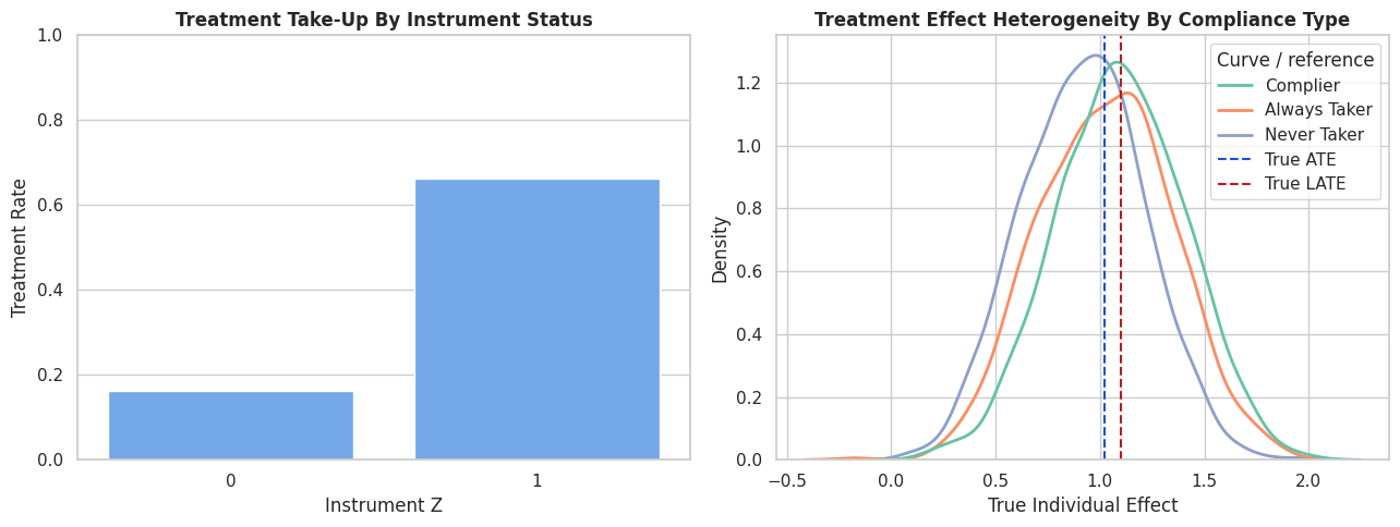
Visualize Compliance And Instrument Take-Up

The left panel shows treatment rates by instrument status. The right panel shows the true individual effects by hidden compliance type.

A binary IV design needs the instrument to create a treatment-rate gap. The effect distribution reminds us that the local target can differ from the population average.

from matplotlib.lines import Line2D

fig, axes = plt.subplots(1, 2, figsize=(13, 5))

takeup = (
    iivm_df.groupby("encouragement")
    .agg(treatment_rate=("feature_exposure", "mean"), n=("feature_exposure", "size"))
    .reset_index()
)
sns.barplot(data=takeup, x="encouragement", y="treatment_rate", color="#60a5fa", ax=axes[0])
axes[0].set_title("Treatment Take-Up By Instrument Status")
axes[0].set_xlabel("Instrument Z")
axes[0].set_ylabel("Treatment Rate")
axes[0].set_ylim(0, 1)

# Seaborn's automatic hue legend can be overwritten after adding Matplotlib reference lines.
# We draw the KDE curves without an automatic legend, then build one combined legend manually.
compliance_order = ["complier", "always_taker", "never_taker"]
compliance_order = [group for group in compliance_order if group in iivm_df["compliance_type"].unique()]
compliance_palette = dict(zip(compliance_order, sns.color_palette("Set2", n_colors=len(compliance_order))))

sns.kdeplot(
    data=iivm_df,
    x="true_tau",
    hue="compliance_type",
    hue_order=compliance_order,
    palette=compliance_palette,
    common_norm=False,
    linewidth=2,
    legend=False,
    ax=axes[1],
)
axes[1].axvline(TRUE_ATE, color="#1d4ed8", linestyle="--", linewidth=1.5)
axes[1].axvline(TRUE_LATE, color="#b91c1c", linestyle="--", linewidth=1.5)
axes[1].set_title("Treatment Effect Heterogeneity By Compliance Type")
axes[1].set_xlabel("True Individual Effect")

legend_handles = [
    Line2D([0], [0], color=compliance_palette[group], linewidth=2, label=group.replace("_", " ").title())
    for group in compliance_order
]
legend_handles.extend(
    [
        Line2D([0], [0], color="#1d4ed8", linestyle="--", linewidth=1.5, label="True ATE"),
        Line2D([0], [0], color="#b91c1c", linestyle="--", linewidth=1.5, label="True LATE"),
    ]
)
axes[1].legend(handles=legend_handles, title="Curve / reference", frameon=True, loc="best")

plt.tight_layout()
fig.savefig(FIGURE_DIR / f"{NOTEBOOK_PREFIX}_compliance_and_take_up.png", dpi=160, bbox_inches="tight")
plt.show()

The instrument creates a clear treatment-rate difference. The effect distributions show why the local effect is not just a technicality; it can be a meaningfully different causal target.

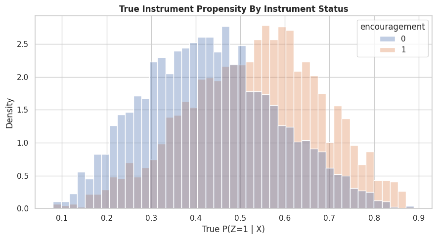
Instrument Overlap

The instrument propensity should not be too close to zero or one. If some covariate profiles almost always receive the same instrument status, there is little local comparison for those profiles.

This cell summarizes the true instrument propensity and displays its distribution by observed instrument status.

instrument_overlap_summary = pd.DataFrame(
    [
        {"diagnostic": "instrument propensity minimum", "value": float(iivm_df["true_instrument_propensity"].min())},
        {"diagnostic": "instrument propensity p05", "value": float(iivm_df["true_instrument_propensity"].quantile(0.05))},
        {"diagnostic": "instrument propensity median", "value": float(iivm_df["true_instrument_propensity"].median())},
        {"diagnostic": "instrument propensity p95", "value": float(iivm_df["true_instrument_propensity"].quantile(0.95))},
        {"diagnostic": "instrument propensity maximum", "value": float(iivm_df["true_instrument_propensity"].max())},
    ]
)
save_table(instrument_overlap_summary, "instrument_overlap_summary")
display(instrument_overlap_summary)

fig, ax = plt.subplots(figsize=(9, 5))
sns.histplot(
    data=iivm_df,
    x="true_instrument_propensity",
    hue="encouragement",
    bins=45,
    stat="density",
    common_norm=False,
    alpha=0.35,
    ax=ax,
)
ax.set_title("True Instrument Propensity By Instrument Status")
ax.set_xlabel("True P(Z=1 | X)")
plt.tight_layout()
fig.savefig(FIGURE_DIR / f"{NOTEBOOK_PREFIX}_instrument_overlap.png", dpi=160, bbox_inches="tight")
plt.show()

	diagnostic	value
0	instrument propensity minimum	0.080000
1	instrument propensity p05	0.218420
2	instrument propensity median	0.475840
3	instrument propensity p95	0.741112
4	instrument propensity maximum	0.889678

The instrument overlap is healthy in this simulation. In real data, poor instrument overlap can make the local effect unstable or limit the population for which the estimate is meaningful.

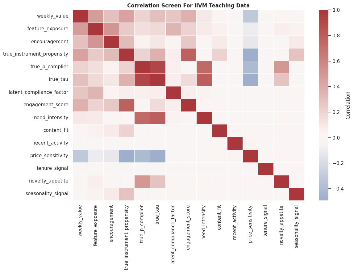
Correlation Screen

The correlation matrix gives a quick view of relationships among outcome, treatment, instrument, compliance probabilities, and controls.

Correlation is not identification. It is just a useful screen before fitting models.

corr_cols = [
    "weekly_value",
    "feature_exposure",
    "encouragement",
    "true_instrument_propensity",
    "true_p_complier",
    "true_tau",
    "latent_compliance_factor",
] + feature_cols
corr_matrix = iivm_df[corr_cols].corr()
save_table(corr_matrix.reset_index().rename(columns={"index": "column"}), "design_correlation_matrix")

fig, ax = plt.subplots(figsize=(12, 9))
sns.heatmap(
    corr_matrix,
    cmap="vlag",
    center=0,
    annot=False,
    linewidths=0.4,
    cbar_kws={"label": "Correlation"},
    ax=ax,
)
ax.set_title("Correlation Screen For IIVM Teaching Data")
plt.tight_layout()
fig.savefig(FIGURE_DIR / f"{NOTEBOOK_PREFIX}_design_correlation_matrix.png", dpi=160, bbox_inches="tight")
plt.show()

The treatment is related to the latent compliance factor, which is why direct treatment comparisons are biased. The instrument is designed to be usable after adjustment for controls.

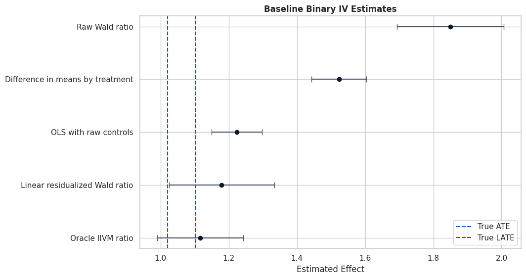
Baseline Estimators

We compare several simple estimators before fitting DoubleML:

• Difference in means by treatment status.
• OLS adjustment using treatment and observed controls.
• Raw Wald ratio using instrument groups without controls.
• Linear residualized Wald ratio.
• Oracle IIVM ratio using the true nuisance functions.

The oracle estimator is available only in this synthetic notebook.

y = iivm_df["weekly_value"].to_numpy()
d = iivm_df["feature_exposure"].to_numpy()
z = iivm_df["encouragement"].to_numpy()
X = iivm_df[feature_cols]

baseline_rows = []
baseline_rows.append(mean_difference_summary(y, d, "Difference in means by treatment", target="direct treatment comparison"))
baseline_rows.append(treatment_ols_summary(iivm_df["weekly_value"], iivm_df[["feature_exposure"] + feature_cols], "feature_exposure", "OLS with raw controls"))
baseline_rows.append(wald_summary(y, d, z, "Raw Wald ratio"))
baseline_rows.append(residualized_wald_summary(y, d, z, X, "Linear residualized Wald ratio"))
baseline_rows.append(
    iivm_ratio_summary(
        y=y,
        d=d,
        z=z,
        g0_hat=iivm_df["true_g0"].to_numpy(),
        g1_hat=iivm_df["true_g1"].to_numpy(),
        m_hat=iivm_df["true_instrument_propensity"].to_numpy(),
        r0_hat=iivm_df["true_r0"].to_numpy(),
        r1_hat=iivm_df["true_r1"].to_numpy(),
        label="Oracle IIVM ratio",
    )
)

baseline_estimates = pd.DataFrame(baseline_rows)
baseline_estimates["true_target"] = np.where(
    baseline_estimates["target"].str.contains("treatment", case=False, na=False),
    TRUE_ATE,
    TRUE_LATE,
)
baseline_estimates.loc[baseline_estimates["estimator"].eq("OLS with raw controls"), "true_target"] = TRUE_ATE
baseline_estimates["bias_vs_target"] = baseline_estimates["theta_hat"] - baseline_estimates["true_target"]
save_table(baseline_estimates, "baseline_estimates")
display(baseline_estimates)

	estimator	target	theta_hat	std_error	ci_95_lower	ci_95_upper	p_value	wald_numerator	wald_denominator	iivm_numerator	iivm_denominator	true_target	bias_vs_target
0	Difference in means by treatment	direct treatment comparison	1.523229	0.040880	1.443103	1.603354	NaN	NaN	NaN	NaN	NaN	1.020535	0.502693
1	OLS with raw controls	observed-control treatment slope	1.223530	0.037648	1.149742	1.297318	1.082914e-231	NaN	NaN	NaN	NaN	1.020535	0.202994
2	Raw Wald ratio	raw Wald LATE-style ratio	1.849634	0.080037	1.692762	2.006506	NaN	0.924632	0.499900	NaN	NaN	1.101928	0.747706
3	Linear residualized Wald ratio	linear residualized Wald ratio	1.178991	0.078897	1.024353	1.333629	NaN	0.124390	0.105505	NaN	NaN	1.101928	0.077064
4	Oracle IIVM ratio	LATE	1.116161	0.064275	0.990182	1.242139	NaN	NaN	NaN	0.527789	0.472861	1.101928	0.014233

Direct treatment comparisons are biased because treatment selection is related to latent compliance factors. The raw Wald ratio is also off because the instrument depends on observed controls. Adjustment matters for the binary IV design.

Baseline Estimate Plot

The plot compares baseline estimates against two reference lines: the true ATE and the true local effect.

The local effect is the correct reference for IV-style rows. The ATE is the reference for direct treatment-comparison rows.

plot_baselines = baseline_estimates.copy().sort_values("theta_hat")
plot_baselines["lower_error"] = plot_baselines["theta_hat"] - plot_baselines["ci_95_lower"]
plot_baselines["upper_error"] = plot_baselines["ci_95_upper"] - plot_baselines["theta_hat"]

fig, ax = plt.subplots(figsize=(10.8, 5.8))
y_pos = np.arange(len(plot_baselines))
ax.errorbar(
    x=plot_baselines["theta_hat"],
    y=y_pos,
    xerr=[plot_baselines["lower_error"], plot_baselines["upper_error"]],
    fmt="o",
    color="#0f172a",
    ecolor="#475569",
    capsize=4,
)
ax.axvline(TRUE_ATE, color="#1d4ed8", linestyle="--", linewidth=1.5, label="True ATE")
ax.axvline(TRUE_LATE, color="#b91c1c", linestyle="--", linewidth=1.5, label="True LATE")
ax.set_yticks(y_pos)
ax.set_yticklabels(plot_baselines["estimator"])
ax.set_xlabel("Estimated Effect")
ax.set_title("Baseline Binary IV Estimates")
ax.legend(loc="lower right")
plt.tight_layout()
fig.savefig(FIGURE_DIR / f"{NOTEBOOK_PREFIX}_baseline_estimates.png", dpi=160, bbox_inches="tight")
plt.show()

The figure shows why IIVM has its own notebook. Binary IV estimates answer a local instrument-induced question, not the same question as a binary-treatment IRM ATE.

Nuisance Learners

DoubleMLIIVM uses three nuisance learner roles:

• ml_g: outcome regression as a function of instrument status and controls.
• ml_m: instrument propensity classifier, P(Z=1 | X).
• ml_r: treatment take-up classifier, P(D=1 | Z, X).

We compare a linear/logistic baseline with gradient boosting. The outcome nuisance is continuous, while the instrument and treatment nuisances are classifiers.

linear_outcome_learner = make_pipeline(
    StandardScaler(),
    LassoCV(cv=3, random_state=RANDOM_STATE, max_iter=5_000),
)
linear_instrument_learner = make_pipeline(
    StandardScaler(),
    LogisticRegressionCV(cv=3, max_iter=2_000, scoring="neg_log_loss", random_state=RANDOM_STATE),
)
linear_treatment_learner = make_pipeline(
    StandardScaler(),
    LogisticRegressionCV(cv=3, max_iter=2_000, scoring="neg_log_loss", random_state=RANDOM_STATE),
)

hgb_outcome_learner = HistGradientBoostingRegressor(
    max_iter=180,
    learning_rate=0.05,
    max_leaf_nodes=24,
    l2_regularization=0.001,
    random_state=RANDOM_STATE,
)
hgb_instrument_learner = HistGradientBoostingClassifier(
    max_iter=180,
    learning_rate=0.05,
    max_leaf_nodes=24,
    l2_regularization=0.001,
    random_state=RANDOM_STATE,
)
hgb_treatment_learner = HistGradientBoostingClassifier(
    max_iter=180,
    learning_rate=0.05,
    max_leaf_nodes=24,
    l2_regularization=0.001,
    random_state=RANDOM_STATE,
)

learner_catalog = pd.DataFrame(
    [
        {"learner_name": "Linear/logistic nuisance set", "use_case": "Transparent baseline; may underfit nonlinear compliance and outcome patterns."},
        {"learner_name": "Gradient-boosted nuisance set", "use_case": "Captures nonlinear instrument, treatment, and outcome nuisance functions."},
    ]
)
save_table(learner_catalog, "learner_catalog")
display(learner_catalog)

	learner_name	use_case
0	Linear/logistic nuisance set	Transparent baseline; may underfit nonlinear c...
1	Gradient-boosted nuisance set	Captures nonlinear instrument, treatment, and ...

The nuisance learners estimate the components of the ratio score. The final target remains the local treatment effect, not the predictive performance itself.

Manual Cross-Fitted IIVM

Before fitting DoubleML, we manually compute the cross-fitted IIVM ratio.

The numerator estimates how the instrument changes the outcome after adjusting for controls. The denominator estimates how the instrument changes treatment after adjusting for controls. Their ratio estimates the local treatment effect.

manual_g0_hat, manual_g1_hat, manual_m_hat, manual_r0_hat, manual_r1_hat = crossfit_iivm_nuisances(
    X=X,
    y=y,
    d=d,
    z=z,
    outcome_learner=hgb_outcome_learner,
    instrument_learner=hgb_instrument_learner,
    treatment_learner=hgb_treatment_learner,
    n_splits=5,
    random_state=RANDOM_STATE,
)

manual_iivm_estimate = pd.DataFrame(
    [
        iivm_ratio_summary(
            y=y,
            d=d,
            z=z,
            g0_hat=manual_g0_hat,
            g1_hat=manual_g1_hat,
            m_hat=manual_m_hat,
            r0_hat=manual_r0_hat,
            r1_hat=manual_r1_hat,
            label="Manual cross-fitted IIVM",
        )
    ]
)
manual_iivm_estimate["true_target"] = TRUE_LATE
manual_iivm_estimate["bias_vs_target"] = manual_iivm_estimate["theta_hat"] - TRUE_LATE
save_table(manual_iivm_estimate, "manual_crossfit_iivm_estimate")
display(manual_iivm_estimate)

	estimator	target	theta_hat	std_error	ci_95_lower	ci_95_upper	p_value	iivm_numerator	iivm_denominator	true_target	bias_vs_target
0	Manual cross-fitted IIVM	LATE	1.185114	0.081281	1.025803	1.344424	NaN	0.549075	0.46331	1.101928	0.083186

The manual cross-fitted ratio is the IIVM idea in plain Python. DoubleML automates the same structure with score management, inference, repeated splits, and diagnostics.

Manual Nuisance Quality

Since this is synthetic data, we can compare cross-fitted nuisance predictions to the true nuisance functions.

Real applications cannot do this. They should use out-of-fold loss, instrument overlap, first-stage diagnostics, and design evidence.

manual_nuisance_quality = pd.DataFrame(
    [
        {
            "nuisance": "g0(X) = E[Y | Z=0, X]",
            "rmse_vs_truth": rmse(iivm_df["true_g0"], manual_g0_hat),
            "mae_vs_truth": float(mean_absolute_error(iivm_df["true_g0"], manual_g0_hat)),
            "correlation_vs_truth": float(np.corrcoef(iivm_df["true_g0"], manual_g0_hat)[0, 1]),
        },
        {
            "nuisance": "g1(X) = E[Y | Z=1, X]",
            "rmse_vs_truth": rmse(iivm_df["true_g1"], manual_g1_hat),
            "mae_vs_truth": float(mean_absolute_error(iivm_df["true_g1"], manual_g1_hat)),
            "correlation_vs_truth": float(np.corrcoef(iivm_df["true_g1"], manual_g1_hat)[0, 1]),
        },
        {
            "nuisance": "m(X) = P(Z=1 | X)",
            "rmse_vs_truth": rmse(iivm_df["true_instrument_propensity"], manual_m_hat),
            "mae_vs_truth": float(mean_absolute_error(iivm_df["true_instrument_propensity"], manual_m_hat)),
            "correlation_vs_truth": float(np.corrcoef(iivm_df["true_instrument_propensity"], manual_m_hat)[0, 1]),
            "auc_for_instrument": float(roc_auc_score(z, manual_m_hat)),
            "log_loss_for_instrument": float(log_loss(z, manual_m_hat)),
        },
        {
            "nuisance": "r0(X) = P(D=1 | Z=0, X)",
            "rmse_vs_truth": rmse(iivm_df["true_r0"], manual_r0_hat),
            "mae_vs_truth": float(mean_absolute_error(iivm_df["true_r0"], manual_r0_hat)),
            "correlation_vs_truth": float(np.corrcoef(iivm_df["true_r0"], manual_r0_hat)[0, 1]),
        },
        {
            "nuisance": "r1(X) = P(D=1 | Z=1, X)",
            "rmse_vs_truth": rmse(iivm_df["true_r1"], manual_r1_hat),
            "mae_vs_truth": float(mean_absolute_error(iivm_df["true_r1"], manual_r1_hat)),
            "correlation_vs_truth": float(np.corrcoef(iivm_df["true_r1"], manual_r1_hat)[0, 1]),
        },
    ]
)
save_table(manual_nuisance_quality, "manual_nuisance_quality")
display(manual_nuisance_quality)

	nuisance	rmse_vs_truth	mae_vs_truth	correlation_vs_truth	auc_for_instrument	log_loss_for_instrument
0	g0(X) = E[Y | Z=0, X]	0.432298	0.332140	0.893133	NaN	NaN
1	g1(X) = E[Y | Z=1, X]	0.472638	0.360051	0.906499	NaN	NaN
2	m(X) = P(Z=1 | X)	0.115957	0.092211	0.807057	0.649979	0.668999
3	r0(X) = P(D=1 | Z=0, X)	0.117598	0.094287	0.394385	NaN	NaN
4	r1(X) = P(D=1 | Z=1, X)	0.155754	0.126420	0.674081	NaN	NaN

The nuisance predictions are useful but imperfect. The local ratio estimate is designed to be less sensitive to small nuisance errors, but weak nuisance quality can still create instability.

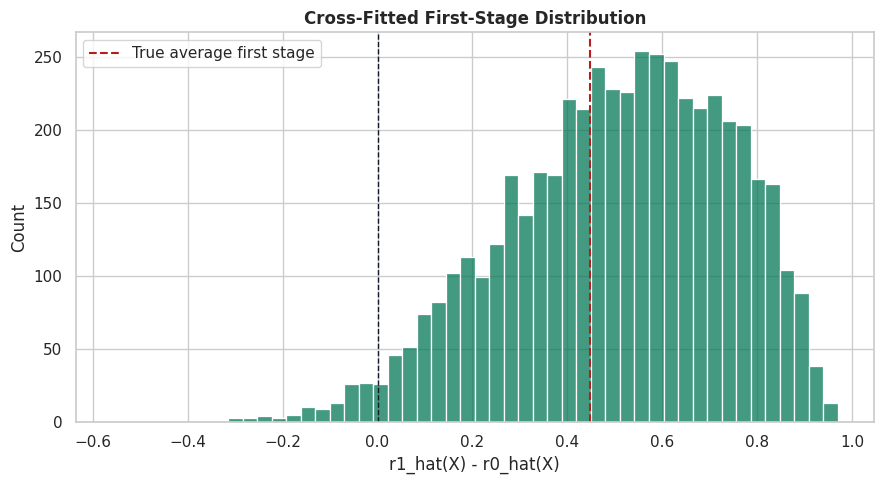
Manual First-Stage Diagnostics

The denominator of the IIVM ratio is the estimated instrument effect on treatment. This is the first stage.

If the denominator is close to zero, the local effect becomes unstable. This cell summarizes the manual cross-fitted first stage.

manual_first_stage = manual_r1_hat - manual_r0_hat
manual_first_stage_summary = pd.DataFrame(
    [
        {
            "diagnostic": "mean first stage r1_hat - r0_hat",
            "value": float(np.mean(manual_first_stage)),
        },
        {"diagnostic": "first-stage p05", "value": float(np.quantile(manual_first_stage, 0.05))},
        {"diagnostic": "first-stage median", "value": float(np.median(manual_first_stage))},
        {"diagnostic": "first-stage p95", "value": float(np.quantile(manual_first_stage, 0.95))},
        {"diagnostic": "share with negative estimated first stage", "value": float(np.mean(manual_first_stage < 0))},
    ]
)
save_table(manual_first_stage_summary, "manual_first_stage_summary")
display(manual_first_stage_summary)

fig, ax = plt.subplots(figsize=(9, 5))
sns.histplot(manual_first_stage, bins=50, color="#047857", alpha=0.75, ax=ax)
ax.axvline(0, color="#111827", linestyle="--", linewidth=1)
ax.axvline(TRUE_FIRST_STAGE, color="#b91c1c", linestyle="--", linewidth=1.5, label="True average first stage")
ax.set_title("Cross-Fitted First-Stage Distribution")
ax.set_xlabel("r1_hat(X) - r0_hat(X)")
ax.legend()
plt.tight_layout()
fig.savefig(FIGURE_DIR / f"{NOTEBOOK_PREFIX}_manual_first_stage_distribution.png", dpi=160, bbox_inches="tight")
plt.show()

	diagnostic	value
0	mean first stage r1_hat - r0_hat	0.505220
1	first-stage p05	0.089992
2	first-stage median	0.528812
3	first-stage p95	0.846567
4	share with negative estimated first stage	0.023400

The first stage is mostly positive and comfortably away from zero on average. That fits the monotonic noncompliance design used in the simulation.

Build The DoubleML Data Object

DoubleMLIIVM needs a DoubleMLData object with:

• outcome column weekly_value;
• treatment column feature_exposure;
• instrument column encouragement;
• observed controls.

The hidden compliance and potential-outcome columns are excluded.

dml_data = DoubleMLData(
    iivm_df[["weekly_value", "feature_exposure", "encouragement"] + feature_cols],
    y_col="weekly_value",
    d_cols="feature_exposure",
    x_cols=feature_cols,
    z_cols="encouragement",
)

backend_summary = pd.DataFrame(
    [
        {"role": "outcome", "columns": dml_data.y_col},
        {"role": "treatment", "columns": ", ".join(dml_data.d_cols)},
        {"role": "instrument", "columns": ", ".join(dml_data.z_cols)},
        {"role": "controls", "columns": ", ".join(dml_data.x_cols)},
        {"role": "number_of_observations", "columns": str(dml_data.n_obs)},
    ]
)
save_table(backend_summary, "doublemldata_backend_summary")
display(backend_summary)

	role	columns
0	outcome	weekly_value
1	treatment	feature_exposure
2	instrument	encouragement
3	controls	engagement_score, need_intensity, content_fit,...
4	number_of_observations	5000

The instrument role is explicit through z_cols. This is the key data-backend difference between IRM and IIVM.

Fit DoubleMLIIVM

We now fit two IIVM specifications:

• a linear/logistic nuisance baseline;
• a gradient-boosted nuisance model.

Both use the default score="LATE" and five-fold cross-fitting.

iivm_model_specs = {
    "Linear nuisance IIVM": {
        "ml_g": linear_outcome_learner,
        "ml_m": linear_instrument_learner,
        "ml_r": linear_treatment_learner,
    },
    "Gradient boosting nuisance IIVM": {
        "ml_g": hgb_outcome_learner,
        "ml_m": hgb_instrument_learner,
        "ml_r": hgb_treatment_learner,
    },
}

iivm_models = {}
for model_name, spec in iivm_model_specs.items():
    model = DoubleMLIIVM(
        dml_data,
        ml_g=clone(spec["ml_g"]),
        ml_m=clone(spec["ml_m"]),
        ml_r=clone(spec["ml_r"]),
        n_folds=5,
        n_rep=1,
        score="LATE",
    )
    model.fit(store_predictions=True)
    iivm_models[model_name] = model
    print(f"Finished: {model_name}")

iivm_summary_rows = []
for model_name, model in iivm_models.items():
    summary = model.summary.reset_index().rename(columns={"index": "treatment"})
    row = summary.iloc[0].to_dict()
    iivm_summary_rows.append(
        {
            "estimator": model_name,
            "treatment": row["treatment"],
            "theta_hat": row["coef"],
            "std_error": row["std err"],
            "t_stat": row["t"],
            "p_value": row["P>|t|"],
            "ci_95_lower": row["2.5 %"],
            "ci_95_upper": row["97.5 %"],
            "true_target": TRUE_LATE,
            "bias_vs_target": row["coef"] - TRUE_LATE,
        }
    )

iivm_summary = pd.DataFrame(iivm_summary_rows)
save_table(iivm_summary, "doubleml_iivm_summary")
display(iivm_summary)

Finished: Linear nuisance IIVM
Finished: Gradient boosting nuisance IIVM

	estimator	treatment	theta_hat	std_error	t_stat	p_value	ci_95_lower	ci_95_upper	true_target	bias_vs_target
0	Linear nuisance IIVM	feature_exposure	1.166017	0.080283	14.523824	8.559872e-48	1.008666	1.323369	1.101928	0.064090
1	Gradient boosting nuisance IIVM	feature_exposure	1.206022	0.081519	14.794455	1.590685e-49	1.046249	1.365795	1.101928	0.104094

The gradient-boosted model is expected to do better because the synthetic compliance and outcome functions are nonlinear. The linear/logistic model is still useful as a transparent baseline.

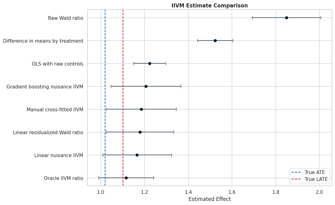
Compare All Estimators

This table combines direct treatment comparisons, Wald-style baselines, the manual cross-fitted IIVM estimate, and DoubleML estimates.

The key comparison is whether an estimator targets the full-population treatment effect or the local instrument-induced effect.

all_estimates = pd.concat(
    [
        baseline_estimates[["estimator", "target", "theta_hat", "std_error", "ci_95_lower", "ci_95_upper", "p_value", "true_target", "bias_vs_target"]],
        manual_iivm_estimate[["estimator", "target", "theta_hat", "std_error", "ci_95_lower", "ci_95_upper", "p_value", "true_target", "bias_vs_target"]],
        iivm_summary.assign(target="LATE")[["estimator", "target", "theta_hat", "std_error", "ci_95_lower", "ci_95_upper", "p_value", "true_target", "bias_vs_target"]],
    ],
    ignore_index=True,
)
all_estimates["abs_bias_vs_target"] = all_estimates["bias_vs_target"].abs()
save_table(all_estimates, "all_estimator_comparison")
display(all_estimates.sort_values("abs_bias_vs_target"))

	estimator	target	theta_hat	std_error	ci_95_lower	ci_95_upper	p_value	true_target	bias_vs_target	abs_bias_vs_target
4	Oracle IIVM ratio	LATE	1.116161	0.064275	0.990182	1.242139	NaN	1.101928	0.014233	0.014233
6	Linear nuisance IIVM	LATE	1.166017	0.080283	1.008666	1.323369	8.559872e-48	1.101928	0.064090	0.064090
3	Linear residualized Wald ratio	linear residualized Wald ratio	1.178991	0.078897	1.024353	1.333629	NaN	1.101928	0.077064	0.077064
5	Manual cross-fitted IIVM	LATE	1.185114	0.081281	1.025803	1.344424	NaN	1.101928	0.083186	0.083186
7	Gradient boosting nuisance IIVM	LATE	1.206022	0.081519	1.046249	1.365795	1.590685e-49	1.101928	0.104094	0.104094
1	OLS with raw controls	observed-control treatment slope	1.223530	0.037648	1.149742	1.297318	1.082914e-231	1.020535	0.202994	0.202994
0	Difference in means by treatment	direct treatment comparison	1.523229	0.040880	1.443103	1.603354	NaN	1.020535	0.502693	0.502693
2	Raw Wald ratio	raw Wald LATE-style ratio	1.849634	0.080037	1.692762	2.006506	NaN	1.101928	0.747706	0.747706

The adjusted local-effect estimators are much closer to the true local target than direct treatment comparisons. The table also shows why the ATE and local target should not be mixed casually.

Estimate Comparison Plot

The figure compares estimates with confidence intervals. The blue line marks the true ATE. The red line marks the true local effect.

IIVM rows should be judged against the red line, not the blue line.

plot_estimates = all_estimates.copy().sort_values("theta_hat")
plot_estimates["lower_error"] = plot_estimates["theta_hat"] - plot_estimates["ci_95_lower"]
plot_estimates["upper_error"] = plot_estimates["ci_95_upper"] - plot_estimates["theta_hat"]

fig, ax = plt.subplots(figsize=(11, 6.8))
y_pos = np.arange(len(plot_estimates))
ax.errorbar(
    x=plot_estimates["theta_hat"],
    y=y_pos,
    xerr=[plot_estimates["lower_error"], plot_estimates["upper_error"]],
    fmt="o",
    color="#0f172a",
    ecolor="#475569",
    capsize=4,
)
ax.axvline(TRUE_ATE, color="#1d4ed8", linestyle="--", linewidth=1.5, label="True ATE")
ax.axvline(TRUE_LATE, color="#b91c1c", linestyle="--", linewidth=1.5, label="True LATE")
ax.set_yticks(y_pos)
ax.set_yticklabels(plot_estimates["estimator"])
ax.set_xlabel("Estimated Effect")
ax.set_title("IIVM Estimate Comparison")
ax.legend(loc="lower right")
plt.tight_layout()
fig.savefig(FIGURE_DIR / f"{NOTEBOOK_PREFIX}_iivm_estimate_comparison.png", dpi=160, bbox_inches="tight")
plt.show()

The plot reinforces the main lesson: binary IV is about the treatment effect for the instrument-induced margin, not necessarily the whole population.

Nuisance Losses

evaluate_learners() reports out-of-fold nuisance losses. For IIVM, the prediction keys are:

• ml_g0: outcome nuisance for Z=0.
• ml_g1: outcome nuisance for Z=1.
• ml_m: instrument propensity nuisance.
• ml_r0: treatment take-up nuisance for Z=0.
• ml_r1: treatment take-up nuisance for Z=1.

These are diagnostics for the nuisance stage, not proofs of instrument validity.

loss_tables = []
for model_name, model in iivm_models.items():
    loss_tables.append(learner_loss_table(model, model_name))

nuisance_losses = pd.concat(loss_tables, ignore_index=True)
save_table(nuisance_losses, "doubleml_nuisance_losses")
display(nuisance_losses)

	model	learner	mean_loss	min_loss	max_loss
0	Linear nuisance IIVM	ml_g0	1.319685	1.319685	1.319685
1	Linear nuisance IIVM	ml_g1	1.356408	1.356408	1.356408
2	Linear nuisance IIVM	ml_m	0.473152	0.473152	0.473152
3	Linear nuisance IIVM	ml_r0	0.365250	0.365250	0.365250
4	Linear nuisance IIVM	ml_r1	0.455724	0.455724	0.455724
5	Gradient boosting nuisance IIVM	ml_g0	1.196010	1.196010	1.196010
6	Gradient boosting nuisance IIVM	ml_g1	1.212799	1.212799	1.212799
7	Gradient boosting nuisance IIVM	ml_m	0.483769	0.483769	0.483769
8	Gradient boosting nuisance IIVM	ml_r0	0.379648	0.379648	0.379648
9	Gradient boosting nuisance IIVM	ml_r1	0.476144	0.476144	0.476144

The loss table helps compare nuisance specifications. It does not answer exclusion, independence, or monotonicity questions.

Extract DoubleML Predictions

We now extract stored predictions from the gradient-boosted IIVM model.

These predictions let us inspect instrument propensity, treatment take-up, first-stage strength, and outcome nuisance quality.

iivm_hgb = iivm_models["Gradient boosting nuisance IIVM"]
dml_g0_hat = prediction_vector(iivm_hgb, "ml_g0")
dml_g1_hat = prediction_vector(iivm_hgb, "ml_g1")
dml_m_hat = np.clip(prediction_vector(iivm_hgb, "ml_m"), 0.02, 0.98)
dml_r0_hat = np.clip(prediction_vector(iivm_hgb, "ml_r0"), 0.01, 0.99)
dml_r1_hat = np.clip(prediction_vector(iivm_hgb, "ml_r1"), 0.01, 0.99)

dml_prediction_quality = pd.DataFrame(
    [
        {"nuisance": "ml_g0 outcome under Z=0", "rmse_vs_truth": rmse(iivm_df["true_g0"], dml_g0_hat), "mae_vs_truth": float(mean_absolute_error(iivm_df["true_g0"], dml_g0_hat)), "correlation_vs_truth": float(np.corrcoef(iivm_df["true_g0"], dml_g0_hat)[0, 1])},
        {"nuisance": "ml_g1 outcome under Z=1", "rmse_vs_truth": rmse(iivm_df["true_g1"], dml_g1_hat), "mae_vs_truth": float(mean_absolute_error(iivm_df["true_g1"], dml_g1_hat)), "correlation_vs_truth": float(np.corrcoef(iivm_df["true_g1"], dml_g1_hat)[0, 1])},
        {"nuisance": "ml_m instrument propensity", "rmse_vs_truth": rmse(iivm_df["true_instrument_propensity"], dml_m_hat), "mae_vs_truth": float(mean_absolute_error(iivm_df["true_instrument_propensity"], dml_m_hat)), "correlation_vs_truth": float(np.corrcoef(iivm_df["true_instrument_propensity"], dml_m_hat)[0, 1]), "auc_for_instrument": float(roc_auc_score(z, dml_m_hat)), "log_loss_for_instrument": float(log_loss(z, dml_m_hat))},
        {"nuisance": "ml_r0 treatment take-up under Z=0", "rmse_vs_truth": rmse(iivm_df["true_r0"], dml_r0_hat), "mae_vs_truth": float(mean_absolute_error(iivm_df["true_r0"], dml_r0_hat)), "correlation_vs_truth": float(np.corrcoef(iivm_df["true_r0"], dml_r0_hat)[0, 1])},
        {"nuisance": "ml_r1 treatment take-up under Z=1", "rmse_vs_truth": rmse(iivm_df["true_r1"], dml_r1_hat), "mae_vs_truth": float(mean_absolute_error(iivm_df["true_r1"], dml_r1_hat)), "correlation_vs_truth": float(np.corrcoef(iivm_df["true_r1"], dml_r1_hat)[0, 1])},
    ]
)
save_table(dml_prediction_quality, "hgb_nuisance_quality_against_truth")
display(dml_prediction_quality)

	nuisance	rmse_vs_truth	mae_vs_truth	correlation_vs_truth	auc_for_instrument	log_loss_for_instrument
0	ml_g0 outcome under Z=0	0.446680	0.342004	0.886067	NaN	NaN
1	ml_g1 outcome under Z=1	0.460292	0.355062	0.912415	NaN	NaN
2	ml_m instrument propensity	0.113231	0.090220	0.816435	0.656847	0.664084
3	ml_r0 treatment take-up under Z=0	0.117381	0.094505	0.385844	NaN	NaN
4	ml_r1 treatment take-up under Z=1	0.154934	0.125704	0.672251	NaN	NaN

The nuisance predictions are good enough for the teaching design, but not perfect. The first-stage nuisance functions are especially important because they form the denominator of the local-effect ratio.

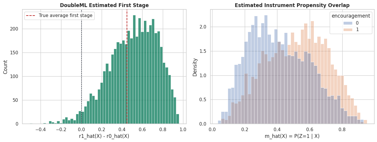
DoubleML First-Stage Diagnostics

This cell summarizes the DoubleML-estimated first stage r1_hat(X) - r0_hat(X).

A strong positive first stage supports relevance and monotonicity-style behavior in the fitted nuisance functions.

dml_first_stage = dml_r1_hat - dml_r0_hat

dml_first_stage_summary = pd.DataFrame(
    [
        {"diagnostic": "mean first stage r1_hat - r0_hat", "value": float(np.mean(dml_first_stage))},
        {"diagnostic": "first-stage p05", "value": float(np.quantile(dml_first_stage, 0.05))},
        {"diagnostic": "first-stage median", "value": float(np.median(dml_first_stage))},
        {"diagnostic": "first-stage p95", "value": float(np.quantile(dml_first_stage, 0.95))},
        {"diagnostic": "share with negative estimated first stage", "value": float(np.mean(dml_first_stage < 0))},
        {"diagnostic": "true average first stage", "value": TRUE_FIRST_STAGE},
    ]
)
save_table(dml_first_stage_summary, "doubleml_first_stage_summary")
display(dml_first_stage_summary)

	diagnostic	value
0	mean first stage r1_hat - r0_hat	0.509133
1	first-stage p05	0.085867
2	first-stage median	0.530857
3	first-stage p95	0.852517
4	share with negative estimated first stage	0.024600
5	true average first stage	0.447774

The estimated first stage is positive on average. A large share of negative estimated first stages would be a warning sign for monotonicity, learner instability, or weak local treatment movement.

First-Stage And Propensity Plots

The left panel shows the estimated first-stage distribution. The right panel shows the estimated instrument propensity by observed instrument status.

Together these plots check relevance and instrument overlap.

fig, axes = plt.subplots(1, 2, figsize=(13, 5))

sns.histplot(dml_first_stage, bins=55, color="#047857", alpha=0.75, ax=axes[0])
axes[0].axvline(0, color="#111827", linestyle="--", linewidth=1)
axes[0].axvline(TRUE_FIRST_STAGE, color="#b91c1c", linestyle="--", linewidth=1.5, label="True average first stage")
axes[0].set_title("DoubleML Estimated First Stage")
axes[0].set_xlabel("r1_hat(X) - r0_hat(X)")
axes[0].legend()

propensity_plot_df = pd.DataFrame({"instrument_propensity": dml_m_hat, "encouragement": z})
sns.histplot(
    data=propensity_plot_df,
    x="instrument_propensity",
    hue="encouragement",
    bins=45,
    stat="density",
    common_norm=False,
    alpha=0.35,
    ax=axes[1],
)
axes[1].set_title("Estimated Instrument Propensity Overlap")
axes[1].set_xlabel("m_hat(X) = P(Z=1 | X)")

plt.tight_layout()
fig.savefig(FIGURE_DIR / f"{NOTEBOOK_PREFIX}_first_stage_and_instrument_overlap.png", dpi=160, bbox_inches="tight")
plt.show()

The first-stage distribution is mostly positive and the instrument propensity has adequate overlap. These are necessary diagnostics, not sufficient proof of IV validity.

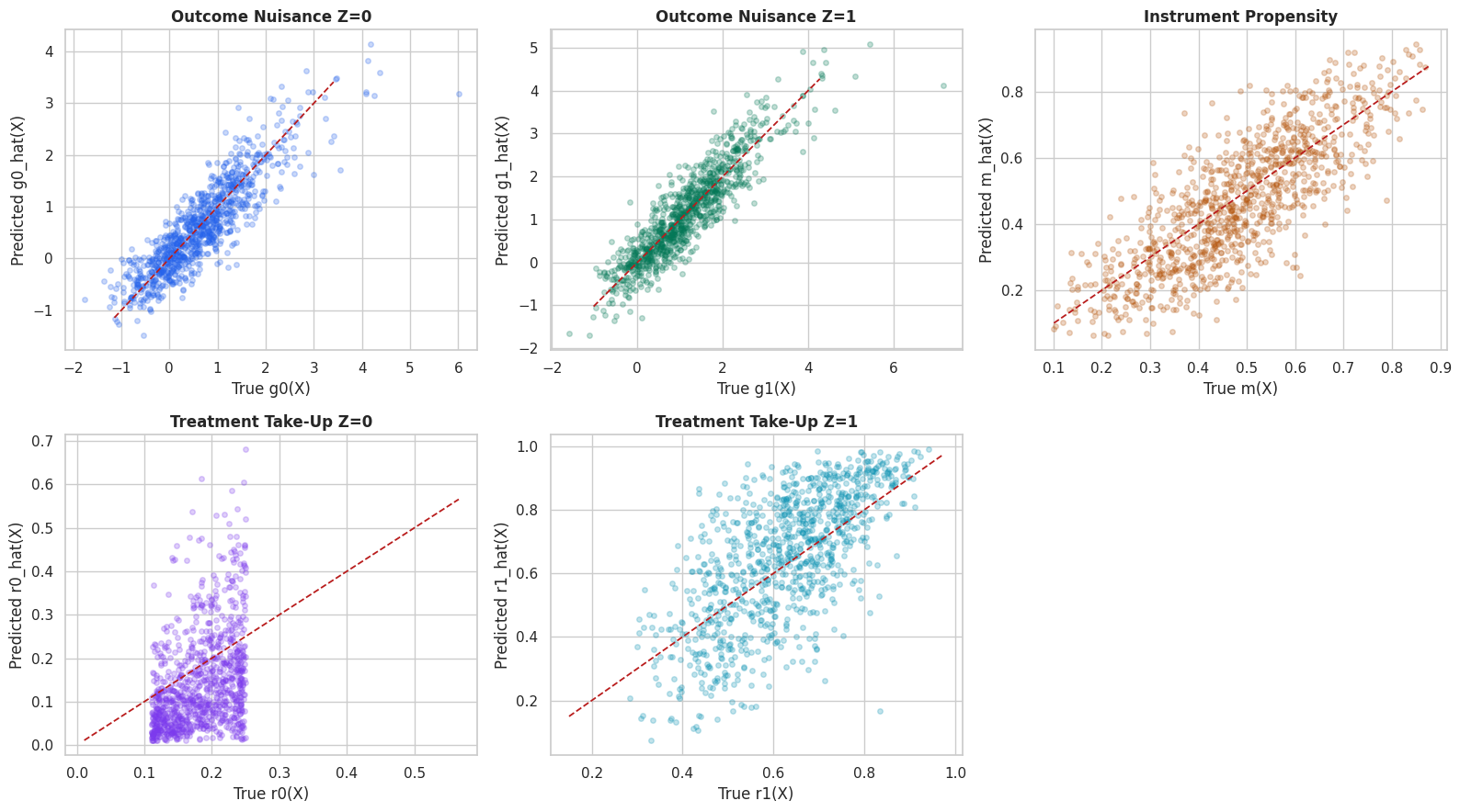
Visual Nuisance Diagnostics

The next figure compares DoubleML’s gradient-boosted nuisance predictions with true synthetic nuisance functions.

In real data, this truth comparison is not possible. The analogous workflow is to inspect out-of-fold losses, calibration, overlap, and first-stage stability.

sample_idx = iivm_df.sample(1_000, random_state=RANDOM_STATE).index

fig, axes = plt.subplots(2, 3, figsize=(16, 9))
plot_specs = [
    (iivm_df["true_g0"].to_numpy(), dml_g0_hat, "Outcome Nuisance Z=0", "True g0(X)", "Predicted g0_hat(X)", "#2563eb"),
    (iivm_df["true_g1"].to_numpy(), dml_g1_hat, "Outcome Nuisance Z=1", "True g1(X)", "Predicted g1_hat(X)", "#047857"),
    (iivm_df["true_instrument_propensity"].to_numpy(), dml_m_hat, "Instrument Propensity", "True m(X)", "Predicted m_hat(X)", "#b45309"),
    (iivm_df["true_r0"].to_numpy(), dml_r0_hat, "Treatment Take-Up Z=0", "True r0(X)", "Predicted r0_hat(X)", "#7c3aed"),
    (iivm_df["true_r1"].to_numpy(), dml_r1_hat, "Treatment Take-Up Z=1", "True r1(X)", "Predicted r1_hat(X)", "#0891b2"),
]

for ax, (truth, pred, title, xlabel, ylabel, color) in zip(axes.ravel(), plot_specs):
    ax.scatter(truth[sample_idx], pred[sample_idx], alpha=0.25, s=16, color=color)
    lower = min(np.quantile(truth, 0.01), np.quantile(pred, 0.01))
    upper = max(np.quantile(truth, 0.99), np.quantile(pred, 0.99))
    ax.plot([lower, upper], [lower, upper], color="#b91c1c", linestyle="--", linewidth=1.3)
    ax.set_title(title)
    ax.set_xlabel(xlabel)
    ax.set_ylabel(ylabel)

axes.ravel()[-1].axis("off")
plt.tight_layout()
fig.savefig(FIGURE_DIR / f"{NOTEBOOK_PREFIX}_doubleml_nuisance_prediction_quality.png", dpi=160, bbox_inches="tight")
plt.show()

The nuisance plots show the model captures the main patterns but smooths some extremes. That is normal for finite-sample machine-learning nuisance estimation.

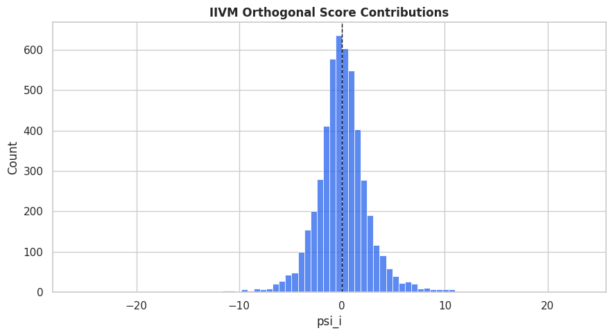
Score Contributions

DoubleML stores orthogonal score contributions in psi. Large tails can signal influential observations, unstable instrument propensities, or weak first-stage regions.

This cell summarizes and plots score contributions from the main gradient-boosted IIVM fit.

psi_values = np.asarray(iivm_hgb.psi)[:, 0, 0]
psi_summary = pd.DataFrame(
    [
        {
            "mean": float(np.mean(psi_values)),
            "std": float(np.std(psi_values, ddof=1)),
            "p01": float(np.quantile(psi_values, 0.01)),
            "p05": float(np.quantile(psi_values, 0.05)),
            "median": float(np.median(psi_values)),
            "p95": float(np.quantile(psi_values, 0.95)),
            "p99": float(np.quantile(psi_values, 0.99)),
        }
    ]
)
save_table(psi_summary, "orthogonal_score_summary")
display(psi_summary)

fig, ax = plt.subplots(figsize=(9, 5))
sns.histplot(psi_values, bins=80, color="#2563eb", alpha=0.75, ax=ax)
ax.axvline(0, color="#111827", linewidth=1, linestyle="--")
ax.set_title("IIVM Orthogonal Score Contributions")
ax.set_xlabel("psi_i")
ax.set_ylabel("Count")
plt.tight_layout()
fig.savefig(FIGURE_DIR / f"{NOTEBOOK_PREFIX}_orthogonal_score_distribution.png", dpi=160, bbox_inches="tight")
plt.show()

	mean	std	p01	p05	median	p95	p99
0	1.080025e-16	2.694336	-6.732241	-3.857392	-0.044926	4.082471	7.634711

The score is centered near zero at the fitted estimate. The tails are moderate for this well-behaved teaching design.

Bootstrap Confidence Interval

DoubleML can compute bootstrap confidence intervals. We run a moderate bootstrap for the main gradient-boosted IIVM model.

As always, bootstrap uncertainty does not validate the instrument assumptions.

iivm_hgb.bootstrap(method="normal", n_rep_boot=500)
bootstrap_ci = iivm_hgb.confint(joint=False, level=0.95).reset_index().rename(columns={"index": "treatment"})
bootstrap_ci["estimator"] = "Gradient boosting nuisance IIVM bootstrap"
save_table(bootstrap_ci, "hgb_bootstrap_confidence_interval")
display(bootstrap_ci)

	treatment	2.5 %	97.5 %	estimator
0	feature_exposure	1.046249	1.365795	Gradient boosting nuisance IIVM bootstrap

The bootstrap interval quantifies sampling uncertainty for the local effect under the fitted design. It should be reported with first-stage and instrument-validity discussion.

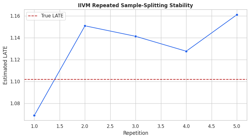
Repeated Sample Splitting

Cross-fitted estimates can move with different fold splits. Repeated sample splitting checks numerical stability.

This cell uses a slightly lighter gradient-boosting configuration so the check remains practical.

repeated_outcome_learner = HistGradientBoostingRegressor(
    max_iter=120,
    learning_rate=0.06,
    max_leaf_nodes=22,
    l2_regularization=0.001,
    random_state=RANDOM_STATE,
)
repeated_instrument_learner = HistGradientBoostingClassifier(
    max_iter=120,
    learning_rate=0.06,
    max_leaf_nodes=22,
    l2_regularization=0.001,
    random_state=RANDOM_STATE,
)
repeated_treatment_learner = HistGradientBoostingClassifier(
    max_iter=120,
    learning_rate=0.06,
    max_leaf_nodes=22,
    l2_regularization=0.001,
    random_state=RANDOM_STATE,
)

iivm_repeated = DoubleMLIIVM(
    dml_data,
    ml_g=clone(repeated_outcome_learner),
    ml_m=clone(repeated_instrument_learner),
    ml_r=clone(repeated_treatment_learner),
    n_folds=5,
    n_rep=5,
    score="LATE",
)
iivm_repeated.fit(store_predictions=False)

split_stability = pd.DataFrame(
    {
        "repetition": np.arange(1, iivm_repeated.all_coef.shape[1] + 1),
        "theta_hat": iivm_repeated.all_coef[0],
        "std_error": iivm_repeated.all_se[0],
    }
)
split_stability["true_late"] = TRUE_LATE
split_stability["bias_vs_true_late"] = split_stability["theta_hat"] - TRUE_LATE
save_table(split_stability, "repeated_sample_split_stability")
display(split_stability)

	repetition	theta_hat	std_error	true_late	bias_vs_true_late
0	1	1.068802	0.075608	1.101928	-0.033125
1	2	1.151013	0.078619	1.101928	0.049085
2	3	1.141402	0.077209	1.101928	0.039474
3	4	1.127719	0.078196	1.101928	0.025792
4	5	1.161182	0.075708	1.101928	0.059254

The repeated estimates should be reasonably close. If they jump around, first-stage instability or nuisance-model sensitivity needs attention.

Split Stability Plot

The next figure shows repeated-split local-effect estimates against the true synthetic local effect.

fig, ax = plt.subplots(figsize=(8.5, 4.8))
sns.lineplot(data=split_stability, x="repetition", y="theta_hat", marker="o", color="#2563eb", ax=ax)
ax.axhline(TRUE_LATE, color="#b91c1c", linestyle="--", linewidth=1.5, label="True LATE")
ax.set_title("IIVM Repeated Sample-Splitting Stability")
ax.set_xlabel("Repetition")
ax.set_ylabel("Estimated LATE")
ax.legend()
plt.tight_layout()
fig.savefig(FIGURE_DIR / f"{NOTEBOOK_PREFIX}_repeated_split_stability.png", dpi=160, bbox_inches="tight")
plt.show()

The estimate is stable across repeated splits in this synthetic design. That supports numerical reliability, not instrument validity by itself.

Subgroup Assumption Variants

DoubleMLIIVM has a subgroups argument for designs where always-takers or never-takers are known to be absent.

Our synthetic data contains both always-takers and never-takers. The default setting is therefore the right one. The next cell fits alternative subgroup restrictions to show that incorrect compliance restrictions can change the estimate.

subgroup_specs = {
    "Default: always and never possible": None,
    "Assume no always-takers": {"always_takers": False, "never_takers": True},
    "Assume no never-takers": {"always_takers": True, "never_takers": False},
    "Assume only compliers": {"always_takers": False, "never_takers": False},
}

subgroup_rows = []
for label, subgroup_config in subgroup_specs.items():
    model = DoubleMLIIVM(
        dml_data,
        ml_g=clone(repeated_outcome_learner),
        ml_m=clone(repeated_instrument_learner),
        ml_r=clone(repeated_treatment_learner),
        n_folds=5,
        n_rep=1,
        score="LATE",
        subgroups=subgroup_config,
    )
    model.fit(store_predictions=False)
    row = model.summary.reset_index().rename(columns={"index": "treatment"}).iloc[0]
    subgroup_rows.append(
        {
            "subgroup_assumption": label,
            "theta_hat": row["coef"],
            "std_error": row["std err"],
            "ci_95_lower": row["2.5 %"],
            "ci_95_upper": row["97.5 %"],
            "true_late": TRUE_LATE,
            "bias_vs_true_late": row["coef"] - TRUE_LATE,
        }
    )

subgroup_comparison = pd.DataFrame(subgroup_rows)
save_table(subgroup_comparison, "subgroup_assumption_comparison")
display(subgroup_comparison)

	subgroup_assumption	theta_hat	std_error	ci_95_lower	ci_95_upper	true_late	bias_vs_true_late
0	Default: always and never possible	1.145934	0.077302	0.994425	1.297442	1.101928	0.044006
1	Assume no always-takers	1.148685	0.078316	0.995190	1.302181	1.101928	0.046758
2	Assume no never-takers	1.170313	0.083855	1.005961	1.334666	1.101928	0.068385
3	Assume only compliers	1.214532	0.085916	1.046140	1.382925	1.101928	0.112605

The subgroup variants are not interchangeable. Use them only when the design genuinely rules out specific compliance types.

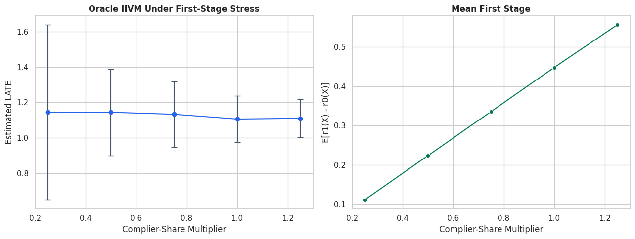
First-Stage Stress Test

A weak instrument creates a small denominator in the IIVM ratio. Even with perfect nuisance functions, weak first stages inflate uncertainty and can make estimates unstable.

This synthetic stress test changes only the complier share and uses oracle nuisance functions so the first-stage issue is isolated.

weak_rows = []
base_tau = true_tau.to_numpy()
base_mu0 = true_mu0.to_numpy()
base_m = true_instrument_propensity.to_numpy()
base_z = encouragement
base_noise = outcome_noise

for multiplier in [0.25, 0.50, 0.75, 1.00, 1.25]:
    pc_stress = np.clip(p_complier.to_numpy() * multiplier, 0.03, 0.90)
    pa_stress = p_always.to_numpy()
    pn_stress = np.clip(1 - pc_stress - pa_stress, 0.03, 0.95)
    total = pc_stress + pa_stress + pn_stress
    pc_stress = pc_stress / total
    pa_stress = pa_stress / total
    pn_stress = pn_stress / total

    draw = rng.uniform(size=N_OBS)
    stress_type = np.where(draw < pa_stress, "always_taker", np.where(draw < pa_stress + pc_stress, "complier", "never_taker"))
    stress_d = np.where(stress_type == "always_taker", 1, np.where(stress_type == "never_taker", 0, base_z))
    stress_y = base_mu0 + base_tau * stress_d + base_noise
    stress_r0 = pa_stress
    stress_r1 = pa_stress + pc_stress
    stress_g0 = base_mu0 + base_tau * stress_r0
    stress_g1 = base_mu0 + base_tau * stress_r1
    stress_late = float(np.mean(pc_stress * base_tau) / np.mean(pc_stress))

    estimate = iivm_ratio_summary(stress_y, stress_d, base_z, stress_g0, stress_g1, base_m, stress_r0, stress_r1, f"first-stage multiplier={multiplier}")
    weak_rows.append(
        {
            "first_stage_multiplier": multiplier,
            "oracle_late": stress_late,
            "mean_first_stage": float(np.mean(stress_r1 - stress_r0)),
            "theta_hat_oracle_iivm": estimate["theta_hat"],
            "std_error_oracle_iivm": estimate["std_error"],
            "ci_95_lower": estimate["ci_95_lower"],
            "ci_95_upper": estimate["ci_95_upper"],
        }
    )

weak_instrument_table = pd.DataFrame(weak_rows)
weak_instrument_table["bias_vs_oracle_late"] = weak_instrument_table["theta_hat_oracle_iivm"] - weak_instrument_table["oracle_late"]
save_table(weak_instrument_table, "weak_instrument_stress_test")
display(weak_instrument_table)

	first_stage_multiplier	oracle_late	mean_first_stage	theta_hat_oracle_iivm	std_error_oracle_iivm	ci_95_lower	ci_95_upper	bias_vs_oracle_late
0	0.25	1.101928	0.111944	1.144375	0.252240	0.649985	1.638765	0.042447
1	0.50	1.101928	0.223887	1.144239	0.124127	0.900950	1.387528	0.042311
2	0.75	1.101928	0.335831	1.132889	0.094093	0.948467	1.317311	0.030961
3	1.00	1.101928	0.447774	1.105957	0.066398	0.975816	1.236097	0.004029
4	1.25	1.098718	0.556162	1.110258	0.054945	1.002567	1.217950	0.011541

As the first stage shrinks, uncertainty grows. A binary IV design with very few compliers cannot support a precise local effect estimate.

Weak-Instrument Plot

The left panel shows oracle local-effect estimates under different first-stage strengths. The right panel shows the denominator of the ratio.

fig, axes = plt.subplots(1, 2, figsize=(13, 5))

axes[0].errorbar(
    x=weak_instrument_table["first_stage_multiplier"],
    y=weak_instrument_table["theta_hat_oracle_iivm"],
    yerr=[
        weak_instrument_table["theta_hat_oracle_iivm"] - weak_instrument_table["ci_95_lower"],
        weak_instrument_table["ci_95_upper"] - weak_instrument_table["theta_hat_oracle_iivm"],
    ],
    fmt="o-",
    color="#2563eb",
    ecolor="#475569",
    capsize=4,
)
axes[0].set_title("Oracle IIVM Under First-Stage Stress")
axes[0].set_xlabel("Complier-Share Multiplier")
axes[0].set_ylabel("Estimated LATE")

sns.lineplot(
    data=weak_instrument_table,
    x="first_stage_multiplier",
    y="mean_first_stage",
    marker="o",
    color="#047857",
    ax=axes[1],
)
axes[1].set_title("Mean First Stage")
axes[1].set_xlabel("Complier-Share Multiplier")
axes[1].set_ylabel("E[r1(X) - r0(X)]")

plt.tight_layout()
fig.savefig(FIGURE_DIR / f"{NOTEBOOK_PREFIX}_weak_instrument_stress_test.png", dpi=160, bbox_inches="tight")
plt.show()

The first stage is the denominator of the estimate. When it gets small, a local-effect estimate can become noisy even if the instrument is valid.

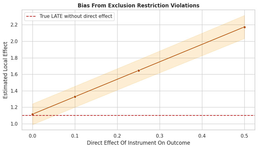
Exclusion-Violation Stress Test

Now we break the exclusion restriction by adding a direct effect of the instrument to the outcome.

The calculation uses oracle nuisance functions so the design violation is isolated. If the instrument affects the outcome directly, the IV ratio no longer recovers the treatment effect for compliers.

exclusion_rows = []
for direct_effect in [0.00, 0.10, 0.25, 0.50]:
    invalid_y = weekly_value + direct_effect * encouragement
    invalid_g0 = true_g0.to_numpy()
    invalid_g1 = true_g1.to_numpy() + direct_effect
    estimate = iivm_ratio_summary(
        invalid_y,
        d,
        z,
        invalid_g0,
        invalid_g1,
        iivm_df["true_instrument_propensity"].to_numpy(),
        iivm_df["true_r0"].to_numpy(),
        iivm_df["true_r1"].to_numpy(),
        f"direct Z effect={direct_effect:.2f}",
    )
    exclusion_rows.append(
        {
            "direct_instrument_effect": direct_effect,
            "theta_hat_oracle_iivm": estimate["theta_hat"],
            "std_error_oracle_iivm": estimate["std_error"],
            "ci_95_lower": estimate["ci_95_lower"],
            "ci_95_upper": estimate["ci_95_upper"],
            "true_late_without_direct_effect": TRUE_LATE,
            "bias_vs_true_late": estimate["theta_hat"] - TRUE_LATE,
        }
    )

exclusion_violation_table = pd.DataFrame(exclusion_rows)
save_table(exclusion_violation_table, "exclusion_violation_stress_test")
display(exclusion_violation_table)

	direct_instrument_effect	theta_hat_oracle_iivm	std_error_oracle_iivm	ci_95_lower	ci_95_upper	true_late_without_direct_effect	bias_vs_true_late
0	0.00	1.116161	0.064275	0.990182	1.242139	1.101928	0.014233
1	0.10	1.327639	0.064680	1.200866	1.454412	1.101928	0.225711
2	0.25	1.644857	0.066289	1.514931	1.774783	1.101928	0.542929
3	0.50	2.173553	0.071402	2.033606	2.313501	1.101928	1.071626

The estimate moves as the direct instrument effect grows. This is the central IV warning: a strong first stage does not protect against a bad exclusion restriction.

Exclusion-Violation Plot

The next figure visualizes how direct instrument effects bias the local-effect estimate.

fig, ax = plt.subplots(figsize=(8.5, 5))
sns.lineplot(
    data=exclusion_violation_table,
    x="direct_instrument_effect",
    y="theta_hat_oracle_iivm",
    marker="o",
    color="#b45309",
    ax=ax,
)
ax.fill_between(
    exclusion_violation_table["direct_instrument_effect"],
    exclusion_violation_table["ci_95_lower"],
    exclusion_violation_table["ci_95_upper"],
    color="#f59e0b",
    alpha=0.18,
)
ax.axhline(TRUE_LATE, color="#b91c1c", linestyle="--", linewidth=1.5, label="True LATE without direct effect")
ax.set_title("Bias From Exclusion Restriction Violations")
ax.set_xlabel("Direct Effect Of Instrument On Outcome")
ax.set_ylabel("Estimated Local Effect")
ax.legend()
plt.tight_layout()
fig.savefig(FIGURE_DIR / f"{NOTEBOOK_PREFIX}_exclusion_violation_stress_test.png", dpi=160, bbox_inches="tight")
plt.show()

This plot shows why instrument design has to be argued carefully. The model can estimate a ratio, but the ratio is causal only under the IV assumptions.

IIVM Compared With IRM

A tempting mistake is to fit a binary-treatment IRM model and treat it as equivalent to IIVM. They target different quantities.

This cell fits a gradient-boosted IRM ATE on the same observed treatment and controls. Because treatment is confounded by compliance-related latent factors, the IRM ATE is not the right design here.

irm_comparison = DoubleMLIRM(
    DoubleMLData(
        iivm_df[["weekly_value", "feature_exposure"] + feature_cols],
        y_col="weekly_value",
        d_cols="feature_exposure",
        x_cols=feature_cols,
    ),
    ml_g=clone(hgb_outcome_learner),
    ml_m=clone(hgb_treatment_learner),
    n_folds=5,
    n_rep=1,
    score="ATE",
)
irm_comparison.fit(store_predictions=True)

irm_vs_iivm = pd.concat(
    [
        irm_comparison.summary.reset_index().rename(columns={"index": "treatment"}).assign(model="IRM ATE on observed treatment", target_reference=TRUE_ATE),
        iivm_hgb.summary.reset_index().rename(columns={"index": "treatment"}).assign(model="IIVM LATE with instrument", target_reference=TRUE_LATE),
    ],
    ignore_index=True,
)
irm_vs_iivm["bias_vs_reference"] = irm_vs_iivm["coef"] - irm_vs_iivm["target_reference"]
save_table(irm_vs_iivm, "irm_vs_iivm_comparison")
display(irm_vs_iivm)

	treatment	coef	std err	t	P>|t|	2.5 %	97.5 %	model	target_reference	bias_vs_reference
0	feature_exposure	1.192215	0.039338	30.307254	9.199046e-202	1.115115	1.269315	IRM ATE on observed treatment	1.020535	0.171679
1	feature_exposure	1.206022	0.081519	14.794455	1.590685e-49	1.046249	1.365795	IIVM LATE with instrument	1.101928	0.104094

The IRM and IIVM estimates answer different questions. In this simulation, the IIVM design is the appropriate response to noncompliance and latent treatment selection.

When IIVM Is The Right Or Wrong Tool

IIVM is useful when:

• treatment is binary;
• instrument is binary;
• noncompliance is central;
• the instrument plausibly shifts treatment but does not directly affect outcome;
• the desired target is a local effect for instrument-responsive units.

IIVM is not enough when:

• the instrument is weak;
• the instrument directly affects the outcome;
• defiers are plausible and monotonicity is not defensible;
• the desired target is the full-population ATE;
• treatment or instrument are continuous rather than binary.

Reporting Checklist

A useful IIVM report should make the local-effect meaning impossible to miss.

The checklist below captures the design and diagnostics needed for binary IV reporting.

reporting_checklist = pd.DataFrame(
    [
        {"item": "Causal question", "status": "Estimate the local effect of feature_exposure on weekly_value for instrument-responsive units."},
        {"item": "Treatment and instrument", "status": "Both feature_exposure and encouragement are binary."},
        {"item": "Target", "status": "LATE, not full-population ATE."},
        {"item": "Instrument relevance", "status": "First-stage take-up diagnostics reported."},
        {"item": "Instrument overlap", "status": "Instrument propensity diagnostics reported."},
        {"item": "Exclusion", "status": "Valid by construction in the synthetic data; requires design evidence in real data."},
        {"item": "Conditional independence", "status": "Valid by construction after X in the synthetic data; requires design evidence in real data."},
        {"item": "Monotonicity", "status": "No defiers by construction; requires design evidence in real data."},
        {"item": "Nuisance learners", "status": "Compared linear/logistic and gradient-boosted nuisance sets."},
        {"item": "Cross-fitting", "status": "Manual ratio and DoubleMLIIVM use cross-fitted nuisance predictions."},
        {"item": "Uncertainty", "status": "Standard errors, confidence intervals, bootstrap interval, and split stability included."},
        {"item": "Stress tests", "status": "Weak first-stage and exclusion-violation stress tests included."},
    ]
)
save_table(reporting_checklist, "iivm_reporting_checklist")
display(reporting_checklist)

	item	status
0	Causal question	Estimate the local effect of feature_exposure ...
1	Treatment and instrument	Both feature_exposure and encouragement are bi...
2	Target	LATE, not full-population ATE.
3	Instrument relevance	First-stage take-up diagnostics reported.
4	Instrument overlap	Instrument propensity diagnostics reported.
5	Exclusion	Valid by construction in the synthetic data; r...
6	Conditional independence	Valid by construction after X in the synthetic...
7	Monotonicity	No defiers by construction; requires design ev...
8	Nuisance learners	Compared linear/logistic and gradient-boosted ...
9	Cross-fitting	Manual ratio and DoubleMLIIVM use cross-fitted...
10	Uncertainty	Standard errors, confidence intervals, bootstr...
11	Stress tests	Weak first-stage and exclusion-violation stres...

The checklist separates estimable diagnostics from assumptions. That separation matters even more for IV than for ordinary observed-control designs.

Report Template

The next cell writes a short markdown report template using the main gradient-boosted IIVM estimate.

This template keeps the local-effect target, first stage, instrument assumptions, and limitations close to the numeric estimate.

main_row = iivm_summary.loc[iivm_summary["estimator"] == "Gradient boosting nuisance IIVM"].iloc[0]
first_stage_mean = dml_first_stage_summary.loc[
    dml_first_stage_summary["diagnostic"] == "mean first stage r1_hat - r0_hat", "value"
].iloc[0]

report_text = f"""
# IIVM Local Effect Estimate Report Template

## Causal Question
Estimate the local effect of `feature_exposure` on `weekly_value` for units whose treatment status is shifted by `encouragement`.

## Target
The target is LATE, not the full-population ATE. The estimate applies to the instrument-responsive margin under the IV assumptions.

## Main Estimate
- Estimated local effect: {main_row['theta_hat']:.4f}
- Standard error: {main_row['std_error']:.4f}
- 95 percent confidence interval: [{main_row['ci_95_lower']:.4f}, {main_row['ci_95_upper']:.4f}]

## First Stage
- Mean estimated first stage: {first_stage_mean:.4f}

## Estimator
The main estimator is `DoubleMLIIVM` with five-fold cross-fitting, histogram gradient-boosted outcome nuisance models, and histogram gradient-boosted classifiers for instrument and treatment take-up nuisance models.

## Diagnostics Included
- Direct treatment comparisons, raw Wald, residualized Wald, oracle ratio, manual cross-fitted IIVM, and DoubleML IIVM comparisons.
- Compliance-type summary for the synthetic teaching data.
- Instrument overlap diagnostics.
- First-stage distribution diagnostics.
- Nuisance learner losses and prediction checks.
- Orthogonal score contribution checks.
- Bootstrap confidence interval.
- Repeated sample-splitting stability.
- Subgroup assumption variants.
- Weak first-stage and exclusion-violation stress tests.

## Required Assumptions
The local effect is causal only if the instrument is relevant, has no direct effect on the outcome, is conditionally independent after controls, satisfies monotonicity, and has adequate overlap. DoubleML estimates the score under these assumptions; it does not establish them.
""".strip()

report_path = REPORT_DIR / f"{NOTEBOOK_PREFIX}_iivm_report_template.md"
report_path.write_text(report_text)
print(report_text)

# IIVM Local Effect Estimate Report Template

## Causal Question
Estimate the local effect of `feature_exposure` on `weekly_value` for units whose treatment status is shifted by `encouragement`.

## Target
The target is LATE, not the full-population ATE. The estimate applies to the instrument-responsive margin under the IV assumptions.

## Main Estimate
- Estimated local effect: 1.2060
- Standard error: 0.0815
- 95 percent confidence interval: [1.0462, 1.3658]

## First Stage
- Mean estimated first stage: 0.5091

## Estimator
The main estimator is `DoubleMLIIVM` with five-fold cross-fitting, histogram gradient-boosted outcome nuisance models, and histogram gradient-boosted classifiers for instrument and treatment take-up nuisance models.

## Diagnostics Included
- Direct treatment comparisons, raw Wald, residualized Wald, oracle ratio, manual cross-fitted IIVM, and DoubleML IIVM comparisons.
- Compliance-type summary for the synthetic teaching data.
- Instrument overlap diagnostics.
- First-stage distribution diagnostics.
- Nuisance learner losses and prediction checks.
- Orthogonal score contribution checks.
- Bootstrap confidence interval.
- Repeated sample-splitting stability.
- Subgroup assumption variants.
- Weak first-stage and exclusion-violation stress tests.

## Required Assumptions
The local effect is causal only if the instrument is relevant, has no direct effect on the outcome, is conditionally independent after controls, satisfies monotonicity, and has adequate overlap. DoubleML estimates the score under these assumptions; it does not establish them.

The report template is deliberately explicit about local-effect meaning. That is the most common place where binary IV results get overclaimed.

Artifact Manifest

The final cell lists every artifact produced by this notebook so the outputs are easy to find later.

artifact_rows = []
for folder, artifact_type in [
    (DATASET_DIR, "dataset"),
    (TABLE_DIR, "table"),
    (FIGURE_DIR, "figure"),
    (REPORT_DIR, "report"),
]:
    for file_path in sorted(folder.glob(f"{NOTEBOOK_PREFIX}_*")):
        artifact_rows.append(
            {
                "artifact_type": artifact_type,
                "file_name": file_path.name,
                "relative_path": str(file_path.relative_to(REPO_ROOT)),
            }
        )

artifact_manifest = pd.DataFrame(artifact_rows)
save_table(artifact_manifest, "artifact_manifest")
display(artifact_manifest)

	artifact_type	file_name	relative_path
0	dataset	06_synthetic_iivm_data.csv	notebooks/tutorials/doubleml/outputs/datasets/...
1	table	06_all_estimator_comparison.csv	notebooks/tutorials/doubleml/outputs/tables/06...
2	table	06_artifact_manifest.csv	notebooks/tutorials/doubleml/outputs/tables/06...
3	table	06_baseline_estimates.csv	notebooks/tutorials/doubleml/outputs/tables/06...
4	table	06_compliance_type_summary.csv	notebooks/tutorials/doubleml/outputs/tables/06...
5	table	06_data_audit.csv	notebooks/tutorials/doubleml/outputs/tables/06...
6	table	06_design_correlation_matrix.csv	notebooks/tutorials/doubleml/outputs/tables/06...
7	table	06_doubleml_first_stage_summary.csv	notebooks/tutorials/doubleml/outputs/tables/06...
8	table	06_doubleml_iivm_summary.csv	notebooks/tutorials/doubleml/outputs/tables/06...
9	table	06_doubleml_nuisance_losses.csv	notebooks/tutorials/doubleml/outputs/tables/06...
10	table	06_doublemldata_backend_summary.csv	notebooks/tutorials/doubleml/outputs/tables/06...
11	table	06_exclusion_violation_stress_test.csv	notebooks/tutorials/doubleml/outputs/tables/06...
12	table	06_field_dictionary.csv	notebooks/tutorials/doubleml/outputs/tables/06...
13	table	06_hgb_bootstrap_confidence_interval.csv	notebooks/tutorials/doubleml/outputs/tables/06...
14	table	06_hgb_nuisance_quality_against_truth.csv	notebooks/tutorials/doubleml/outputs/tables/06...
15	table	06_iivm_reporting_checklist.csv	notebooks/tutorials/doubleml/outputs/tables/06...
16	table	06_instrument_overlap_summary.csv	notebooks/tutorials/doubleml/outputs/tables/06...
17	table	06_irm_vs_iivm_comparison.csv	notebooks/tutorials/doubleml/outputs/tables/06...
18	table	06_learner_catalog.csv	notebooks/tutorials/doubleml/outputs/tables/06...
19	table	06_manual_crossfit_iivm_estimate.csv	notebooks/tutorials/doubleml/outputs/tables/06...
20	table	06_manual_first_stage_summary.csv	notebooks/tutorials/doubleml/outputs/tables/06...
21	table	06_manual_nuisance_quality.csv	notebooks/tutorials/doubleml/outputs/tables/06...
22	table	06_orthogonal_score_summary.csv	notebooks/tutorials/doubleml/outputs/tables/06...
23	table	06_package_versions.csv	notebooks/tutorials/doubleml/outputs/tables/06...
24	table	06_repeated_sample_split_stability.csv	notebooks/tutorials/doubleml/outputs/tables/06...
25	table	06_subgroup_assumption_comparison.csv	notebooks/tutorials/doubleml/outputs/tables/06...
26	table	06_target_summary.csv	notebooks/tutorials/doubleml/outputs/tables/06...
27	table	06_weak_instrument_stress_test.csv	notebooks/tutorials/doubleml/outputs/tables/06...
28	figure	06_baseline_estimates.png	notebooks/tutorials/doubleml/outputs/figures/0...
29	figure	06_compliance_and_take_up.png	notebooks/tutorials/doubleml/outputs/figures/0...
30	figure	06_design_correlation_matrix.png	notebooks/tutorials/doubleml/outputs/figures/0...
31	figure	06_doubleml_nuisance_prediction_quality.png	notebooks/tutorials/doubleml/outputs/figures/0...
32	figure	06_exclusion_violation_stress_test.png	notebooks/tutorials/doubleml/outputs/figures/0...
33	figure	06_first_stage_and_instrument_overlap.png	notebooks/tutorials/doubleml/outputs/figures/0...
34	figure	06_iivm_design_dag.png	notebooks/tutorials/doubleml/outputs/figures/0...
35	figure	06_iivm_estimate_comparison.png	notebooks/tutorials/doubleml/outputs/figures/0...
36	figure	06_instrument_overlap.png	notebooks/tutorials/doubleml/outputs/figures/0...
37	figure	06_manual_first_stage_distribution.png	notebooks/tutorials/doubleml/outputs/figures/0...
38	figure	06_orthogonal_score_distribution.png	notebooks/tutorials/doubleml/outputs/figures/0...
39	figure	06_repeated_split_stability.png	notebooks/tutorials/doubleml/outputs/figures/0...
40	figure	06_weak_instrument_stress_test.png	notebooks/tutorials/doubleml/outputs/figures/0...
41	report	06_iivm_report_template.md	notebooks/tutorials/doubleml/outputs/reports/0...

The IIVM notebook is complete. The next natural topic is difference-in-differences, where the identifying assumption shifts from observed-control adjustment or instruments to parallel trends.