This notebook is a full tutorial on DoubleMLPLIV, the partially linear instrumental-variable model for a continuous treatment.
The previous notebook handled a continuous treatment under observed-control adjustment. Here we make the problem harder: even after controlling for observed covariates, the treatment is still endogenous because an unobserved factor affects both treatment and outcome. A valid instrument can recover the treatment effect by using treatment variation induced by the instrument.
The notebook is intentionally theory-heavy because IV designs are easy to misuse. The package can estimate an IV model, but it cannot prove that the instrument is valid.
Learning Goals
By the end of this notebook, you should be able to:
Explain why observed-control adjustment can fail when treatment is endogenous.
State the PLIV model and the role of the instrument.
Distinguish instrument relevance, exclusion, and conditional independence.
Understand the DoubleMLPLIV nuisance roles: ml_l, ml_m, and ml_r.
Manually compute the residualized IV estimand using cross-fitted nuisance predictions.
Fit DoubleMLPLIV with linear and nonlinear nuisance learners.
Diagnose first-stage strength and residual treatment variation.
Explain why weak or invalid instruments can make IV estimates unstable or biased.
Why We Need IV
Observed-control methods such as PLR assume that, after conditioning on X, the remaining treatment variation is usable for causal estimation. That assumption fails when there is an unobserved variable U that affects both the treatment D and the outcome Y.
An instrument Z is a variable that shifts treatment but does not directly shift the outcome except through treatment. If the instrument is valid, it can isolate a source of treatment variation that is not contaminated by the unobserved confounder.
The IV logic is powerful, but fragile. A weak instrument can create noisy estimates. An invalid instrument can create precise estimates of the wrong quantity.
where l_0(X) = E[Y | X], m_0(X) = E[Z | X], and r_0(X) = E[D | X].
The Three Main IV Assumptions
A credible IV design usually needs at least these conditions:
Relevance: the instrument changes the treatment after adjusting for controls.
Exclusion: the instrument affects the outcome only through the treatment.
Conditional independence: after adjusting for controls, the instrument is not related to unobserved outcome shocks.
Only relevance can be directly screened in the data through first-stage diagnostics. Exclusion and conditional independence require design arguments, domain knowledge, institutional details, or randomized encouragement.
Runtime Note
This notebook fits several cross-fitted nuisance models and a repeated-split check. On a typical laptop, the full notebook should take roughly two to four minutes.
The weak-instrument and invalid-instrument sections use fast oracle-style residual calculations rather than repeatedly fitting large machine-learning models. That keeps the cautionary simulations readable and quick.
Setup
This cell prepares the notebook environment. It creates output folders, makes matplotlib cache writes local to the tutorial folder, imports the scientific Python stack, and records package versions.
The path logic supports running the notebook either from the repository root or from the tutorial folder.
The package table is saved with the notebook outputs. IV estimates can change slightly with learner implementations, random splits, and numerical defaults, so version tracking is part of the reproducibility story.
Helper Functions
The next cell defines utilities for saving tables, computing OLS summaries, residualizing variables, computing residualized IV estimates, and extracting DoubleML diagnostics.
The residualized IV function is especially important because it makes the PLIV score concrete: estimate the slope using the covariance between residualized instrument and residualized outcome divided by the covariance between residualized instrument and residualized treatment.
The manual IV helper uses the same core moment that the PLIV partialling-out score uses. This makes the DoubleML output easier to trust because we can reproduce the core calculation ourselves.
Draw The IV Design
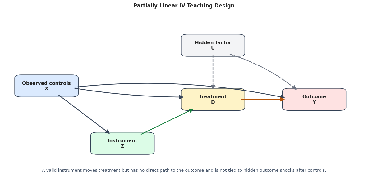
The figure below shows the teaching design.
X affects the instrument, treatment, and outcome. Z affects D. D affects Y. The hidden factor U affects both D and Y, creating endogeneity that ordinary observed-control adjustment cannot remove.
The instrument is useful only if the dashed hidden path does not also connect to Z after conditioning on X, and if Z has no direct path to Y except through D.
from matplotlib.patches import FancyBboxPatch, FancyArrowPatchnodes = {"X": {"xy": (0.12, 0.58), "label": "Observed controls\nX", "color": "#dbeafe"},"Z": {"xy": (0.33, 0.24), "label": "Instrument\nZ", "color": "#dcfce7"},"D": {"xy": (0.58, 0.50), "label": "Treatment\nD", "color": "#fef3c7"},"Y": {"xy": (0.86, 0.50), "label": "Outcome\nY", "color": "#fee2e2"},"U": {"xy": (0.58, 0.82), "label": "Hidden factor\nU", "color": "#f3f4f6"},}edge_specs = [ ("X", "Z", "#334155", "solid", 0.00), ("X", "D", "#334155", "solid", 0.04), ("X", "Y", "#334155", "solid", -0.08), ("Z", "D", "#15803d", "solid", 0.00), ("D", "Y", "#b45309", "solid", 0.00), ("U", "D", "#6b7280", "dashed", 0.00), ("U", "Y", "#6b7280", "dashed", -0.10),]fig, ax = plt.subplots(figsize=(12, 6.2))ax.set_axis_off()box_w, box_h =0.14, 0.095def edge_endpoint(source_xy, target_xy, from_source=True):"""Return a point just outside the source or target box boundary.""" x0, y0 = source_xy x1, y1 = target_xy dx, dy = x1 - x0, y1 - y0 scale =1.0/max(abs(dx) / (box_w /2), abs(dy) / (box_h /2))if from_source:return (x0 + dx * scale *1.08, y0 + dy * scale *1.08)return (x1 - dx * scale *1.12, y1 - dy * scale *1.12)for spec in nodes.values(): x, y = spec["xy"] rect = FancyBboxPatch( (x - box_w /2, y - box_h /2), box_w, box_h, boxstyle="round,pad=0.018", facecolor=spec["color"], edgecolor="#334155", linewidth=1.2, zorder=3, ) ax.add_patch(rect) ax.text(x, y, spec["label"], ha="center", va="center", fontsize=11, fontweight="bold", zorder=4)for start, end, color, style, rad in edge_specs: start_xy = edge_endpoint(nodes[start]["xy"], nodes[end]["xy"], from_source=True) end_xy = edge_endpoint(nodes[start]["xy"], nodes[end]["xy"], from_source=False) arrow = FancyArrowPatch( start_xy, end_xy, arrowstyle="-|>", mutation_scale=20, linewidth=1.8, color=color, linestyle=style, connectionstyle=f"arc3,rad={rad}", zorder=5, ) ax.add_patch(arrow)ax.text(0.50,0.08,"A valid instrument moves treatment but has no direct path to the outcome and is not tied to hidden outcome shocks after controls.", ha="center", va="center", fontsize=10, color="#475569",)ax.set_title("Partially Linear IV Teaching Design", pad=18)plt.tight_layout()fig.savefig(FIGURE_DIR /f"{NOTEBOOK_PREFIX}_pliv_design_dag.png", dpi=160, bbox_inches="tight")plt.show()
The diagram is the causal story the estimator depends on. The analysis can screen relevance and stability, but the exclusion and independence arrows require an argument outside the fitted model.
Create A Teaching Dataset With Endogeneity
We now simulate a dataset where treatment is endogenous.
The hidden variable latent_demand_shock affects both treatment and outcome. It is not included in the observed controls. This means PLR-style adjustment with X alone will remain biased.
The instrument encouragement_score affects treatment and is generated so that its residual variation is not tied to the hidden demand shock. That makes it valid in this synthetic setup.
The hidden columns are included only because this is a teaching simulation. In an applied dataset, the hidden demand shock would be exactly the problem: it would affect treatment and outcome, but we would not observe it.
Field Dictionary
This table documents the role of every important column. The ml_m and ml_r distinction is worth repeating: in PLIV, ml_m predicts the instrument and ml_r predicts the treatment.
The instrument is intentionally kept out of the control set. In DoubleML, it belongs in z_cols, not in x_cols. Mixing these roles would change the represented design.
Basic Data Audit
Before modeling, we check missingness, scale, and variation for outcome, treatment, instrument, and controls.
For IV work, low instrument variation or an instrument with many missing values is an immediate concern. A model can still run, but the design would be weak.
The hidden demand shock is correlated with treatment and outcome, which creates endogeneity. The instrument is correlated with treatment, which supports relevance in this synthetic setup.
Visualize Endogeneity And Relevance
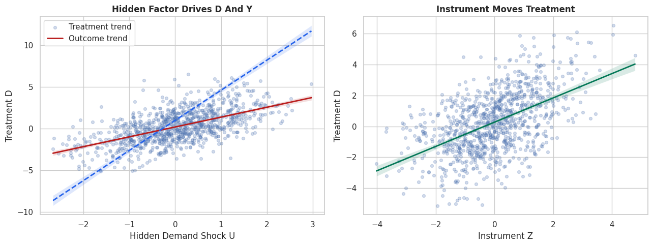
The next figure shows two important relationships.
The left panel shows that the hidden demand shock affects both treatment and outcome. The right panel shows that the instrument moves treatment.
In real data, the left panel is unavailable because the confounder is unobserved. The point of IV is to handle precisely that situation, provided the instrument is credible.
This is the central tension: treatment is confounded by an unobserved factor, but the instrument creates an additional source of treatment variation.
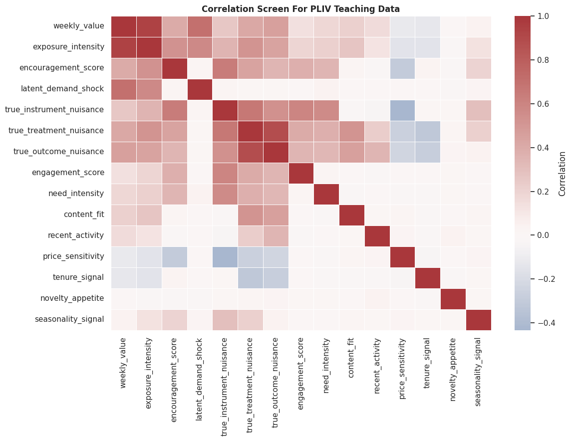
Design Correlation Matrix
The correlation matrix is not a causal proof, but it helps us inspect the data-generating structure.
The hidden teaching columns are included here only so the simulation is transparent. In real data, we would use observed variables and separate design evidence for the unobserved threats.
The instrument has a visible relationship with treatment. The hidden factor has a visible relationship with treatment and outcome. That is why observed-control adjustment alone will struggle.
Baseline Estimators
We now compare several estimators:
Naive OLS: regress outcome on treatment only.
Observed-control OLS: adjust for X but ignore the hidden confounder.
Naive IV: use the instrument without adjusting for X.
Linear residualized IV: residualize outcome, treatment, and instrument on X linearly, then use IV.
Oracle residualized IV: use the true nuisance functions from the simulation.
The oracle estimator is not available in real data. It is included only to show the target behavior when nuisance functions are known.
The OLS estimates are biased because the hidden factor remains in the treatment-outcome relationship. The IV estimates use instrument-induced variation and move much closer to the true effect.
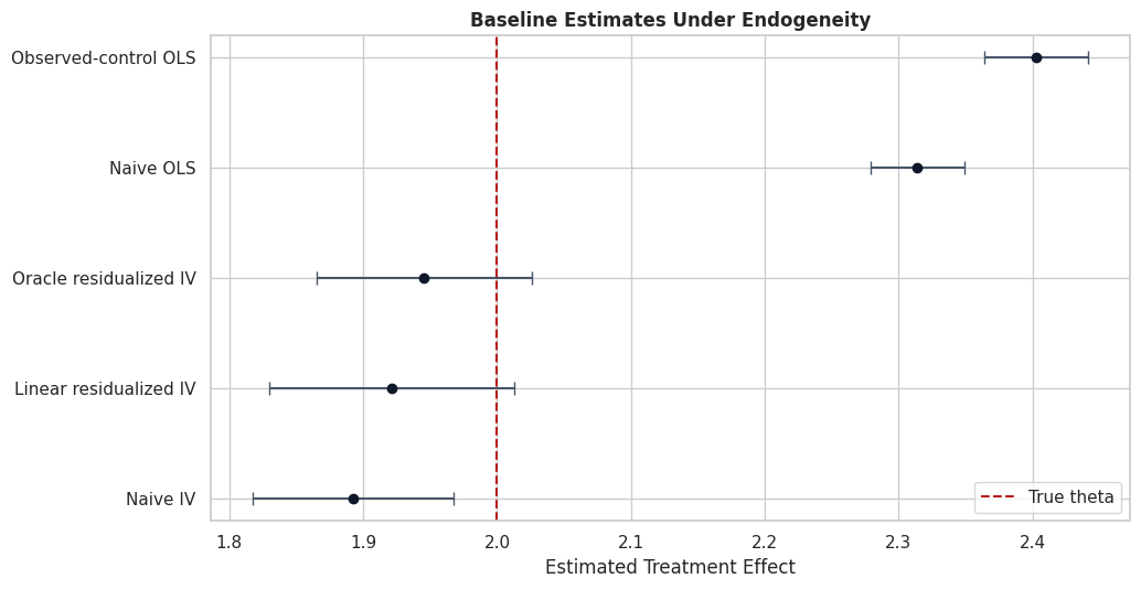
Baseline Estimate Plot
This plot shows the baseline estimates with confidence intervals. The dashed red line marks the true effect from the simulation.
In real data, there is no true-effect line. The same plot would instead compare credible specifications and uncertainty intervals.
The visual contrast is the reason for using IV. Observed controls help, but they cannot remove a hidden common cause. The instrument changes which treatment variation identifies the slope.
First-Stage Relevance Screen
A relevant instrument must predict treatment after adjusting for controls. Here we use a linear residualized first-stage screen:
residualize treatment on X;
residualize instrument on X;
regress residualized treatment on residualized instrument.
This is not the only possible first-stage diagnostic, but it gives an intuitive relevance check.
first_stage_table = pd.DataFrame( [ first_stage_summary(d, z, "Raw first stage"), first_stage_summary(linear_d_resid, linear_z_resid, "Linear residualized first stage"), first_stage_summary(oracle_d_resid, oracle_z_resid, "Oracle residualized first stage"), ])save_table(first_stage_table, "first_stage_relevance_screen")display(first_stage_table)
diagnostic
first_stage_slope
first_stage_r2
first_stage_f_stat
residual_corr_z_d
0
Raw first stage
0.827788
0.279944
971.175003
0.529097
1
Linear residualized first stage
0.796256
0.207512
654.100047
0.455535
2
Oracle residualized first stage
0.795393
0.206756
651.092278
0.454704
The residualized first stage is strong in this synthetic design. In applied IV work, weak first-stage evidence should make the estimate a warning sign rather than a final answer.
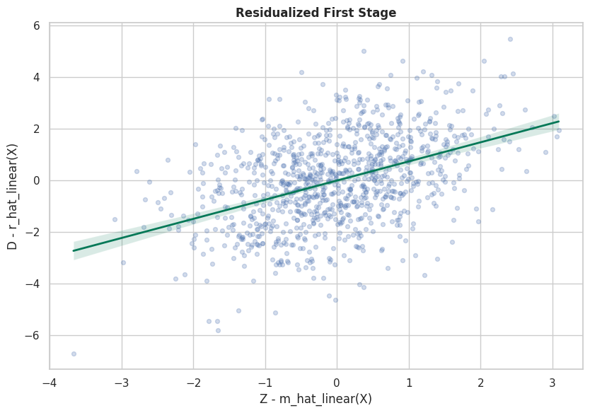
Residual First-Stage Plot
This figure shows the relationship between residualized instrument and residualized treatment after linear adjustment for X.
The slope is the first-stage relationship. If this cloud were almost flat, the instrument would provide little usable treatment variation.
The nuisance learners are not estimating the causal effect directly. They remove predictable parts of outcome, treatment, and instrument so that the final IV moment uses residualized variation.
Manual Cross-Fitted PLIV
Before using the package, we manually compute the partialling-out PLIV estimate with cross-fitted nuisance predictions.
The steps are:
Predict Y from X out of fold.
Predict Z from X out of fold.
Predict D from X out of fold.
Form residuals for outcome, instrument, and treatment.
Estimate the IV slope from residualized variables.
This is the PLIV moment in plain Python. DoubleML automates this logic and adds inference, repeated sample splitting, score management, and a consistent model API.
Manual Nuisance Quality
Because this is synthetic data, we can compare cross-fitted nuisance predictions with the true nuisance functions.
In real data, we cannot compute these columns. We would rely on out-of-fold predictive diagnostics, residual plots, first-stage checks, and the IV design argument.
The nuisance functions are not perfect, especially because treatment and outcome contain hidden shocks. Orthogonal IV scoring is designed to reduce sensitivity to nuisance estimation error, but poor nuisance quality can still increase instability.
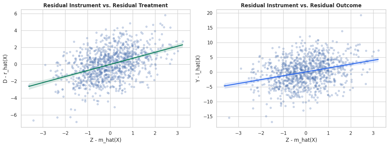
Manual Residual IV Plot
The next plot shows the residualized instrument-treatment relationship and the residualized instrument-outcome relationship.
PLIV uses the part of the instrument that remains after adjusting for controls. The treatment effect is identified by how that residualized instrument shifts residualized outcome through residualized treatment.
This data object is the executable version of the IV design. If the instrument were accidentally placed in x_cols instead of z_cols, the model would no longer represent the intended IV estimand.
Fit DoubleMLPLIV
We now fit DoubleMLPLIV with two nuisance specifications:
regularized linear nuisances;
gradient-boosted nuisances.
Both use the partialling-out score and five-fold cross-fitting.
Finished: Linear nuisance PLIV
Finished: Gradient boosting nuisance PLIV
estimator
treatment
theta_hat
std_error
t_stat
p_value
ci_95_lower
ci_95_upper
true_theta
bias_vs_truth
0
Linear nuisance PLIV
exposure_intensity
1.921241
0.046800
41.052195
0.0
1.829515
2.012967
2.0
-0.078759
1
Gradient boosting nuisance PLIV
exposure_intensity
1.873601
0.047531
39.418577
0.0
1.780442
1.966760
2.0
-0.126399
The PLIV estimates use residualized instrument variation rather than raw treatment variation. In this synthetic design, that should reduce the endogeneity bias that affected OLS.
Compare All Estimators
The comparison table combines OLS, manual IV, oracle IV, and DoubleML PLIV estimates.
The most important comparison is not package versus package. It is raw treatment variation versus instrument-induced treatment variation.
The IV-based estimates are closer to the true effect than OLS because they avoid the hidden treatment-outcome path. The remaining differences are sampling noise and nuisance-model error.
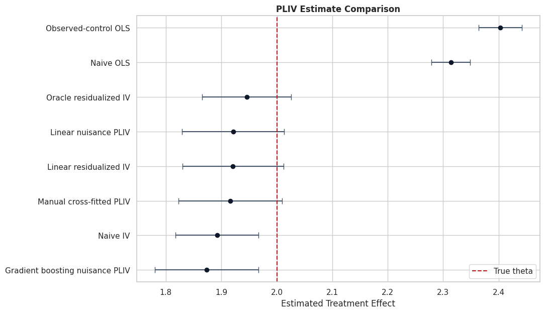
Estimate Comparison Plot
This figure summarizes the estimator comparison. The dashed red line is the true effect in the simulation.
In real data, the goal would be to compare credible specifications and make assumptions explicit rather than to match a known truth.
The instrument nuisance is easier to predict than the treatment nuisance because treatment contains the hidden demand shock. This mirrors real IV settings where treatment can be hard to predict fully from observed controls.
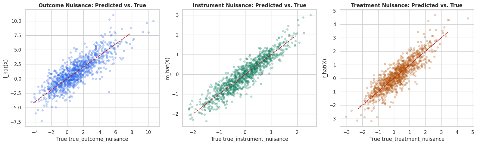
Visual Nuisance Diagnostics
This figure compares predicted nuisance functions to the true nuisance functions. The middle panel is especially useful because it reinforces that ml_m predicts the instrument in PLIV.
The plots show useful but imperfect nuisance recovery. That is the normal DML setting: flexible learners help estimate nuisance structure, while orthogonal scores reduce first-order sensitivity to nuisance errors.
Residual Diagnostics From DoubleML
The residualized instrument and treatment are central to PLIV. If the residualized instrument has little relationship with residualized treatment, the IV estimate will be unstable.
This cell summarizes the residual distributions and the residualized first stage from the gradient-boosted DoubleML fit.
The residualized first stage remains strong. This supports the relevance condition after flexible adjustment for observed controls.
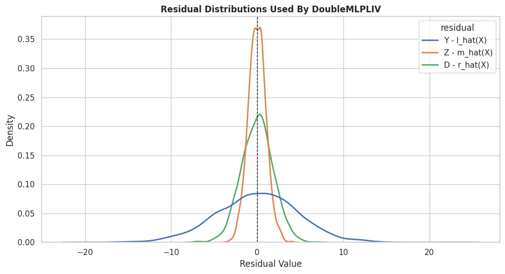
Residual Distribution Plot
This plot shows the residualized outcome, instrument, and treatment distributions from the DoubleML fit.
The instrument residual should have meaningful spread. The treatment residual should also have meaningful spread. If either collapses, the IV moment becomes fragile.
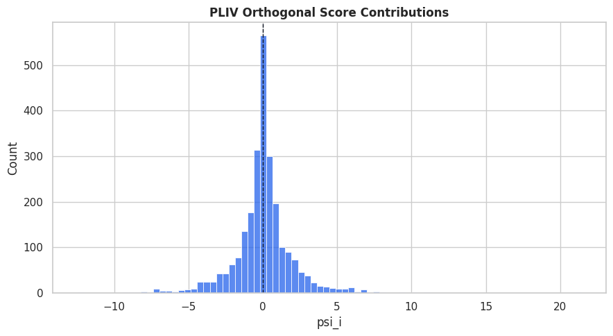
The score is centered near zero, as expected at the fitted estimate. The tail behavior is another reminder that IV uncertainty can be sensitive to residual instrument strength.
Partialling-Out Score vs. IV-Type Score
DoubleMLPLIV supports both partialling out and IV-type scores. The default partialling-out score estimates l, m, and r. The IV-type score also uses ml_g, a nuisance learner for a transformed outcome equation.
This cell fits an IV-type score as a specification comparison. The goal is not to declare one score universally better; it is to show how to run and compare the supported score variants.
The score variants are close in this synthetic example. In applied work, large differences across reasonable scores or learners would deserve investigation before writing a conclusion.
Bootstrap Confidence Interval
DoubleML can compute bootstrap-based confidence intervals. Bootstrap tools are especially useful when there are multiple parameters or joint inference needs.
Here we run a moderate bootstrap for the main gradient-boosted PLIV fit.
The bootstrap interval quantifies sampling uncertainty under the fitted IV design. It does not validate the exclusion restriction or remove weak-instrument concerns.
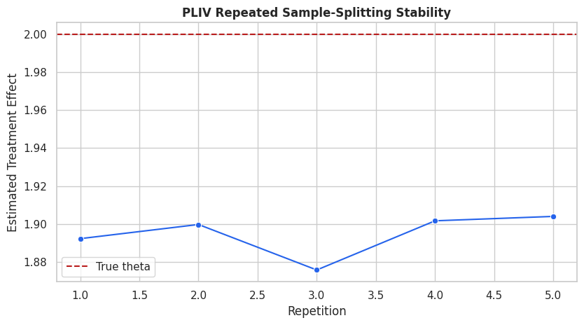
Repeated Sample Splitting
Cross-fitted estimates can move slightly with different fold splits. Repeated sample splitting checks whether the result is stable across split draws.
This cell uses a lighter learner so the repeated-split check remains practical.
The estimate is reasonably stable across fold repetitions here. This is a numerical stability check, not a substitute for instrument validity.
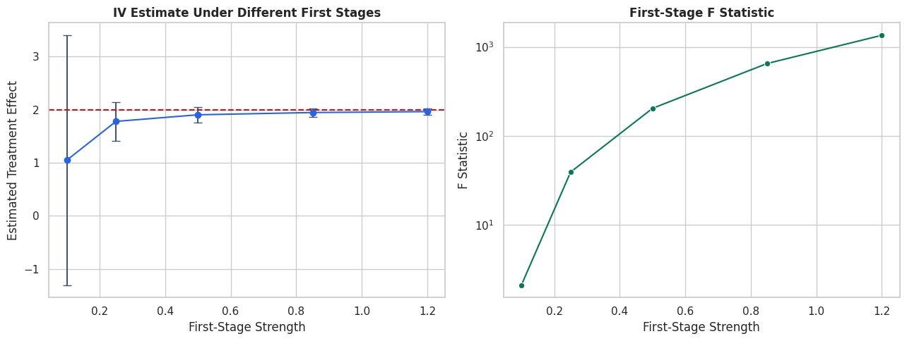
Weak-Instrument Stress Test
A weak instrument has little residual relationship with treatment. When the first-stage denominator becomes small, IV estimates can become noisy and unreliable.
This synthetic stress test changes only the first-stage strength and uses the true nuisance functions to isolate the weak-instrument issue from nuisance-model error.
As the first stage gets weaker, the residual instrument-treatment relationship shrinks and the standard error grows. This is why first-stage diagnostics belong in every IV report.
Weak-Instrument Plot
The next figure shows how first-stage strength changes uncertainty. The point estimates may move around because finite samples are noisy, but the uncertainty pattern is the main lesson.
The weak-instrument problem is not a software problem. It is a design problem. Better learners do not create instrument relevance when the instrument barely moves treatment.
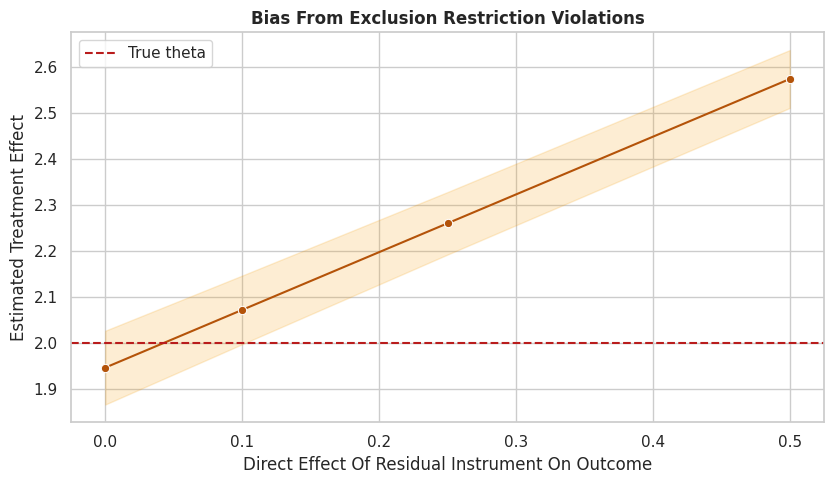
Exclusion-Violation Stress Test
Now we keep the first stage fixed but add a direct effect from the residual instrument to the outcome. This breaks the exclusion restriction.
The calculation again uses true nuisance functions so we can isolate the design failure. If the instrument directly affects the outcome, IV estimates can be biased even when the first stage is strong.
The estimate moves as the exclusion violation grows. This is the hard part of IV: the most important assumption cannot usually be verified by a first-stage plot.
Exclusion-Violation Plot
The next figure visualizes how a direct instrument-outcome path changes the estimated treatment effect.
This is why IV writeups need a design story. A strong first stage plus a violated exclusion restriction can still produce a misleading result.
When PLIV Is The Right Or Wrong Tool
PLIV is useful when:
treatment is continuous;
unobserved confounding is plausible after observed-control adjustment;
a credible instrument shifts treatment;
the target can be summarized as a constant linear treatment effect.
PLIV is not the right tool when:
the treatment is binary and compliance is central, where an interactive IV model may be more natural;
no credible instrument exists;
the instrument barely moves treatment;
the instrument directly affects the outcome;
the treatment effect is too heterogeneous for a constant-slope summary to be meaningful.
Reporting Checklist
A useful PLIV report should make the instrument argument as visible as the estimate.
This checklist turns the notebook into a reusable applied workflow.
reporting_checklist = pd.DataFrame( [ {"item": "Causal question", "status": "Estimate effect of exposure_intensity on weekly_value using instrument-induced variation."}, {"item": "Treatment type", "status": "Continuous treatment; PLIV constant-slope estimand is appropriate for the teaching design."}, {"item": "Instrument role", "status": "encouragement_score assigned through z_cols, not included as an ordinary control."}, {"item": "Relevance", "status": "Residualized first-stage diagnostics reported."}, {"item": "Exclusion", "status": "Valid by construction in synthetic data; requires design evidence in real data."}, {"item": "Conditional independence", "status": "Valid by construction after X in synthetic data; requires design evidence in real data."}, {"item": "Nuisance learners", "status": "Compared regularized linear and gradient-boosted nuisances."}, {"item": "Cross-fitting", "status": "Used five folds and manually demonstrated cross-fitted residualized IV."}, {"item": "Uncertainty", "status": "Reported standard errors, confidence intervals, and a bootstrap interval."}, {"item": "Stability", "status": "Checked repeated sample splitting."}, {"item": "Cautions", "status": "Included weak-instrument and exclusion-violation stress tests."}, ])save_table(reporting_checklist, "pliv_reporting_checklist")display(reporting_checklist)
item
status
0
Causal question
Estimate effect of exposure_intensity on weekl...
1
Treatment type
Continuous treatment; PLIV constant-slope esti...
2
Instrument role
encouragement_score assigned through z_cols, n...
3
Relevance
Residualized first-stage diagnostics reported.
4
Exclusion
Valid by construction in synthetic data; requi...
5
Conditional independence
Valid by construction after X in synthetic dat...
6
Nuisance learners
Compared regularized linear and gradient-boost...
7
Cross-fitting
Used five folds and manually demonstrated cros...
8
Uncertainty
Reported standard errors, confidence intervals...
9
Stability
Checked repeated sample splitting.
10
Cautions
Included weak-instrument and exclusion-violati...
The checklist separates estimable diagnostics from assumptions that need a design argument. That separation is the heart of honest IV reporting.
Report Template
The next cell writes a short markdown report template using the main gradient-boosted PLIV estimate.
This is not meant to be copied blindly. It is a structure for explaining the estimate, the instrument, the first stage, and the limitations.
main_row = pliv_summary.loc[pliv_summary["estimator"] =="Gradient boosting nuisance PLIV"].iloc[0]first_stage_row = dml_first_stage.iloc[0]report_text =f"""# PLIV Effect Estimate Report Template## Causal QuestionEstimate the effect of `exposure_intensity` on `weekly_value` using `encouragement_score` as an instrument.## Design LogicThe concern is that unobserved factors may affect both treatment and outcome. The instrument is intended to shift treatment while affecting the outcome only through treatment after adjusting for observed controls.## EstimatorThe main estimator is `DoubleMLPLIV` with the partialling-out score, five-fold cross-fitting, and histogram gradient-boosting nuisance learners.## Main Estimate- Estimated effect: {main_row['theta_hat']:.4f}- Standard error: {main_row['std_error']:.4f}- 95 percent confidence interval: [{main_row['ci_95_lower']:.4f}, {main_row['ci_95_upper']:.4f}]## First Stage- Residualized first-stage slope: {first_stage_row['first_stage_slope']:.4f}- Residualized first-stage F statistic: {first_stage_row['first_stage_f_stat']:.2f}- Residual instrument-treatment correlation: {first_stage_row['residual_corr_z_d']:.4f}## Diagnostics Included- OLS, naive IV, residualized IV, oracle IV, and DoubleML PLIV comparisons.- First-stage relevance screen.- Manual cross-fitted PLIV calculation.- Nuisance learner RMSE checks.- Residual distribution and score contribution checks.- Score variant comparison.- Bootstrap confidence interval.- Repeated sample-splitting stability.- Weak-instrument and exclusion-violation stress tests.## Required AssumptionsThe estimate relies on instrument relevance, exclusion, and conditional independence after controls. Relevance is screened in the data. Exclusion and conditional independence require design evidence and cannot be established by DoubleML alone.""".strip()report_path = REPORT_DIR /f"{NOTEBOOK_PREFIX}_pliv_report_template.md"report_path.write_text(report_text)print(report_text)
# PLIV Effect Estimate Report Template

## Causal Question
Estimate the effect of `exposure_intensity` on `weekly_value` using `encouragement_score` as an instrument.

## Design Logic
The concern is that unobserved factors may affect both treatment and outcome. The instrument is intended to shift treatment while affecting the outcome only through treatment after adjusting for observed controls.

## Estimator
The main estimator is `DoubleMLPLIV` with the partialling-out score, five-fold cross-fitting, and histogram gradient-boosting nuisance learners.

## Main Estimate
- Estimated effect: 1.8736
- Standard error: 0.0475
- 95 percent confidence interval: [1.7804, 1.9668]

## First Stage
- Residualized first-stage slope: 0.7953
- Residualized first-stage F statistic: 618.22
- Residual instrument-treatment correlation: 0.4454

## Diagnostics Included
- OLS, naive IV, residualized IV, oracle IV, and DoubleML PLIV comparisons.
- First-stage relevance screen.
- Manual cross-fitted PLIV calculation.
- Nuisance learner RMSE checks.
- Residual distribution and score contribution checks.
- Score variant comparison.
- Bootstrap confidence interval.
- Repeated sample-splitting stability.
- Weak-instrument and exclusion-violation stress tests.

## Required Assumptions
The estimate relies on instrument relevance, exclusion, and conditional independence after controls. Relevance is screened in the data. Exclusion and conditional independence require design evidence and cannot be established by DoubleML alone.
The report template keeps the instrument assumptions next to the numeric estimate. That is essential for IV work: the model output and the instrument story must travel together.
Artifact Manifest
The final cell lists the artifacts produced by this notebook so they are easy to find later.
The PLIV notebook is complete. The next natural topic is the interactive regression model for binary treatments, where propensity scores and potential-outcome nuisance functions become central.