DoubleML Tutorial 03: Partially Linear Regression PLR
This notebook is a full tutorial on the DoubleMLPLR model: the partially linear regression design for a continuous treatment.
The goal is not just to call an API. The goal is to understand the causal target, the nuisance functions, the orthogonal score, the cross-fitting logic, the diagnostics, and the reporting caveats that make the estimate credible.
We will work with a synthetic teaching dataset where the true treatment effect is known. That lets us see exactly what goes wrong with naive regression and why residualization plus orthogonalization is useful. In a real application the true effect is not known, so the same workflow would focus on design assumptions, nuisance diagnostics, uncertainty, and robustness rather than checking against a known answer.
Learning Goals
By the end of this notebook, you should be able to:
State the PLR estimand in words and equations.
Explain why the treatment and outcome nuisance functions matter.
Recognize the difference between naive prediction adjustment and Neyman-orthogonal estimation.
Manually compute the residual-on-residual PLR estimate using cross-fitted nuisance predictions.
Fit DoubleMLPLR with flexible learners.
Read coefficients, standard errors, confidence intervals, nuisance losses, and split-stability diagnostics.
Write a short, honest report for a PLR estimate.
Where PLR Fits
DoubleMLPLR is appropriate when the treatment is continuous or can be reasonably treated as a continuous dose, and the causal effect is represented by a constant slope after adjusting for observed covariates.
Examples of PLR-style questions include:
What is the average effect of one additional unit of exposure intensity on a future user outcome, after adjusting for user history?
What is the effect of a pricing, ranking, or messaging intensity score on demand, after adjusting for baseline demand predictors?
What is the effect of a continuous operational intervention on a downstream metric, after adjusting for the variables that influenced the intervention?
The model is called partially linear because the treatment enters linearly, while the relationship between covariates and both the outcome and treatment can be flexible and nonlinear.
The PLR Model
The standard partially linear regression model is:
\[
Y = \theta_0 D + g_0(X) + \zeta, \quad E[\zeta \mid D, X] = 0
\]
and the treatment equation is:
\[
D = m_0(X) + V, \quad E[V \mid X] = 0
\]
Here:
Y is the outcome.
D is the continuous treatment or dose.
X is the set of observed controls.
theta_0 is the target causal slope.
g_0(X) is the outcome nuisance function.
m_0(X) is the treatment nuisance function.
V is the part of treatment variation not explained by controls.
The identifying idea is that, after controlling for X, the remaining variation in D behaves as good-as-random for estimating the slope on Y. DoubleML does not make that assumption true; the analyst has to defend it through the causal design.
Orthogonal Score Intuition
The partialling-out score used in this notebook is:
where l(X) = E[Y | X], m(X) = E[D | X], and eta = (l, m) are nuisance functions.
This score creates two residuals:
treatment residual: D - m(X)
outcome residual: Y - l(X)
Then it estimates theta from the relationship between the residualized outcome and residualized treatment.
The important theoretical feature is Neyman orthogonality: small first-order errors in the nuisance functions have little first-order impact on the treatment-effect estimate. That is what allows flexible machine-learning models to be used for nuisance estimation without directly turning prediction bias into treatment-effect bias.
Practical Runtime Note
This notebook fits several cross-fitted nuisance models. On a typical laptop, the full notebook should take roughly one to three minutes. The heaviest cells are the gradient-boosting PLR fits and the manual cross-fitting cell.
The examples are intentionally moderate in size. They are large enough to show the behavior of the estimators but small enough to keep the tutorial easy to rerun.
Setup
This cell prepares the notebook environment. It creates output folders, makes matplotlib cache writes local to the tutorial folder, imports the scientific Python stack, and records package versions for reproducibility.
The path logic supports two common ways of running the notebook: from the repository root or directly from the tutorial folder.
The package table is more than bookkeeping. In causal ML tutorials, reproducibility depends on both the statistical design and the software versions, especially when cross-fitting and tree-based learners are involved.
Helper Functions
The next cell defines small helper functions used throughout the notebook. Keeping these utilities in one place makes the analysis cells easier to read.
The functions do four jobs:
Save tables with consistent names.
Compute regression summaries for simple OLS baselines.
Compute PLR estimates from residuals.
Pull DoubleML predictions and learner losses into tidy tables.
def save_table(df, name):"""Save a dataframe to the tutorial table directory and return it for display.""" path = TABLE_DIR /f"{NOTEBOOK_PREFIX}_{name}.csv" df.to_csv(path, index=False)return dfdef regression_summary(y, X, treatment_col, label):"""Fit an HC1-robust OLS model and return the treatment coefficient row.""" X_design = sm.add_constant(X, has_constant="add") fit = sm.OLS(y, X_design).fit(cov_type="HC1") row = fit.summary2().tables[1].loc[treatment_col]return {"estimator": label,"theta_hat": row["Coef."],"std_error": row["Std.Err."],"ci_95_lower": row["[0.025"],"ci_95_upper": row["0.975]"],"p_value": row["P>|z|"],"r_squared": fit.rsquared, }def plr_from_residuals(y_resid, d_resid, label):"""Compute the partialling-out estimate and large-sample standard error.""" y_resid = np.asarray(y_resid) d_resid = np.asarray(d_resid) n_obs =len(y_resid) theta_hat =float(np.sum(d_resid * y_resid) / np.sum(d_resid **2)) score = d_resid * (y_resid - theta_hat * d_resid) derivative =-np.mean(d_resid **2) std_error =float(np.sqrt(np.mean(score **2) / (derivative **2* n_obs)))return {"estimator": label,"theta_hat": theta_hat,"std_error": std_error,"ci_95_lower": theta_hat -1.96* std_error,"ci_95_upper": theta_hat +1.96* std_error, }def prediction_vector(doubleml_model, learner_key):"""Extract the first treatment and first repetition prediction vector.""" arr = np.asarray(doubleml_model.predictions[learner_key])if arr.ndim !=3:raiseValueError(f"Expected a 3D prediction array, got shape {arr.shape}")return arr[:, 0, 0]def learner_loss_table(doubleml_model, model_label):"""Convert DoubleML learner evaluation arrays into a tidy dataframe.""" losses = doubleml_model.evaluate_learners() rows = []for learner_name, values in losses.items(): arr = np.asarray(values) rows.append( {"model": model_label,"learner": learner_name,"mean_rmse": float(np.mean(arr)),"min_rmse": float(np.min(arr)),"max_rmse": float(np.max(arr)), } )return pd.DataFrame(rows)def rmse(y_true, y_pred):returnfloat(np.sqrt(mean_squared_error(y_true, y_pred)))
These helpers are intentionally transparent. A strong applied notebook should make the statistical calculations visible enough that the reader can connect the package output to the underlying estimand.
Create A Teaching Dataset
We now simulate a continuous-treatment causal problem. The covariates are named like ordinary product or marketplace features, but the data are synthetic.
The treatment is exposure_intensity. It is not randomly assigned. It depends on observed user/context features through a nonlinear treatment rule. The outcome is weekly_value, and it depends on both the treatment and the same observed features.
Because the outcome nuisance function is correlated with the treatment rule, a naive regression of outcome on treatment will be biased.
The saved dataset includes both the observable columns and hidden teaching columns such as the true nuisance functions. In real data those true nuisance functions are not available. They are included here only so we can check whether each estimator behaves as expected.
Field Dictionary
Before modeling, we document the columns. This is a small habit with a large payoff: causal workflows depend on roles. A column is not just a feature; it may be an outcome, treatment, pre-treatment control, generated diagnostic, or hidden simulation quantity.
The controls are all pre-treatment by construction. That matters because PLR adjusts for X; including post-treatment variables would change the estimand and can block part of the treatment effect.
Basic Data Audit
The next cell checks shape, missingness, basic moments, and the observed correlation between treatment and outcome.
A data audit does not prove identification, but it catches ordinary failures before we spend time interpreting an estimator: missing values, constant variables, implausible scales, or a treatment with too little variation.
audit_rows = []for column in ["weekly_value", "exposure_intensity"] + feature_cols: s = plr_df[column] audit_rows.append( {"column": column,"missing_rate": float(s.isna().mean()),"mean": float(s.mean()),"std": float(s.std()),"min": float(s.min()),"p05": float(s.quantile(0.05)),"median": float(s.median()),"p95": float(s.quantile(0.95)),"max": float(s.max()),"n_unique": int(s.nunique()), } )data_audit = pd.DataFrame(audit_rows)save_table(data_audit, "data_audit")display(data_audit)observed_corr = plr_df[["weekly_value", "exposure_intensity"]].corr().iloc[0, 1]print(f"Observed treatment-outcome correlation: {observed_corr:.3f}")print(f"True theta used in the simulation: {TRUE_THETA:.2f}")
column
missing_rate
mean
std
min
p05
median
p95
max
n_unique
0
weekly_value
0.0
1.430433
4.539450
-13.456512
-5.672829
1.376231
9.125022
19.897151
3000
1
exposure_intensity
0.0
0.379496
1.621467
-4.835908
-2.230475
0.389084
3.092460
7.074104
3000
2
engagement_score
0.0
-0.002931
1.014648
-3.659392
-1.684926
0.006120
1.604898
4.013439
3000
3
need_intensity
0.0
-0.018741
1.006393
-3.484637
-1.669852
-0.019327
1.662892
3.150908
3000
4
content_fit
0.0
0.012325
0.984224
-3.987716
-1.600982
0.024807
1.592880
3.600337
3000
5
recent_activity
0.0
-0.001487
1.003650
-3.573864
-1.600296
0.017822
1.671128
3.653308
3000
6
price_sensitivity
0.0
-0.001699
0.991457
-3.747414
-1.676108
0.026963
1.591078
3.417551
3000
7
tenure_signal
0.0
0.022647
1.021025
-3.586747
-1.670351
0.035436
1.706382
3.667511
3000
8
novelty_appetite
0.0
-0.000142
0.976362
-4.044650
-1.571103
-0.020953
1.613075
3.230977
3000
9
seasonality_signal
0.0
0.006351
1.011668
-3.272317
-1.633538
0.013726
1.678134
3.620951
3000
Observed treatment-outcome correlation: 0.935
True theta used in the simulation: 1.75
The treatment and outcome are strongly related in the raw data. That relationship is not automatically causal because the treatment was assigned based on covariates that also affect the outcome.
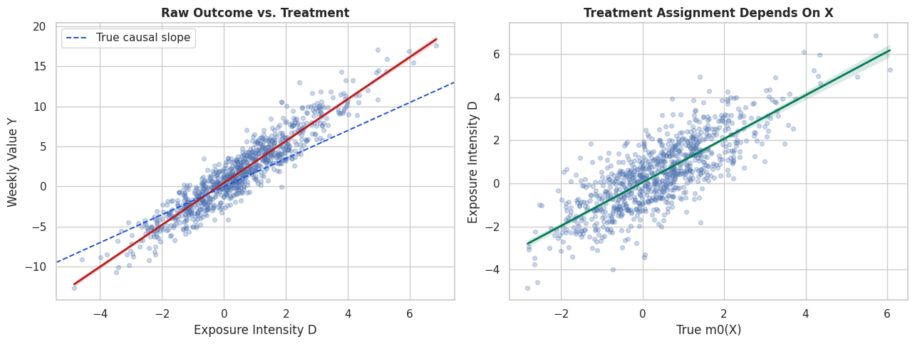
Visualize The Confounding Pattern
This figure has two panels.
The left panel shows the observed treatment-outcome relationship. The right panel shows how treatment intensity relates to the true treatment nuisance function, which is the part of treatment explained by observed controls.
In real data we would not know the true nuisance function, but the simulation lets us see the confounding mechanism directly.
The raw slope mixes two signals: the causal effect of treatment and the non-causal association created by the assignment rule. PLR tries to remove the part of treatment and outcome explained by controls before estimating the slope.
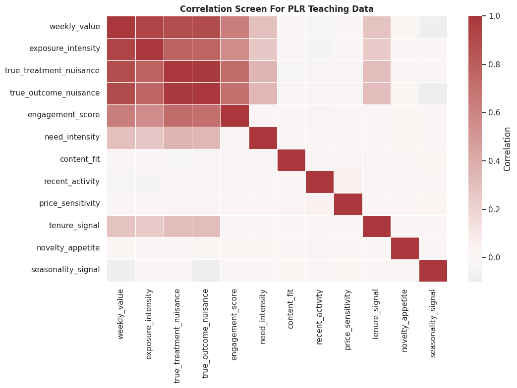
Design Correlation Matrix
The correlation matrix gives a quick, imperfect view of the data-generating structure. Linear correlations will miss some nonlinear relationships, but they still help us see which variables are visibly tied to treatment and outcome.
The hidden nuisance columns are included here for teaching. In a real dataset, this plot would use only observed variables and engineered pre-treatment features.
The matrix shows why pure outcome prediction is not enough. Several controls are related to treatment and outcome, so a treatment-effect estimator has to separate assignment-driven variation from residual treatment variation.
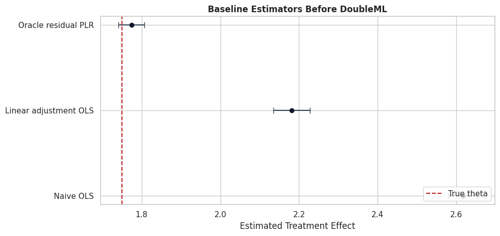
Baseline Estimators
Before fitting DoubleML, we build simple baselines:
Naive OLS: regress outcome only on treatment.
Linear adjustment OLS: regress outcome on treatment and raw controls.
Oracle residual PLR: residualize using the true nuisance functions from the simulation.
The oracle estimator is not available in real data. It is here to show the target behavior when residualization is perfect.
The naive estimate is pulled away from the true effect because treatment intensity is higher for units with stronger expected outcomes. Linear adjustment improves the situation only if the raw linear controls approximate the true nuisance functions well. The oracle residual estimate shows the ideal target when the residualization step is correct.
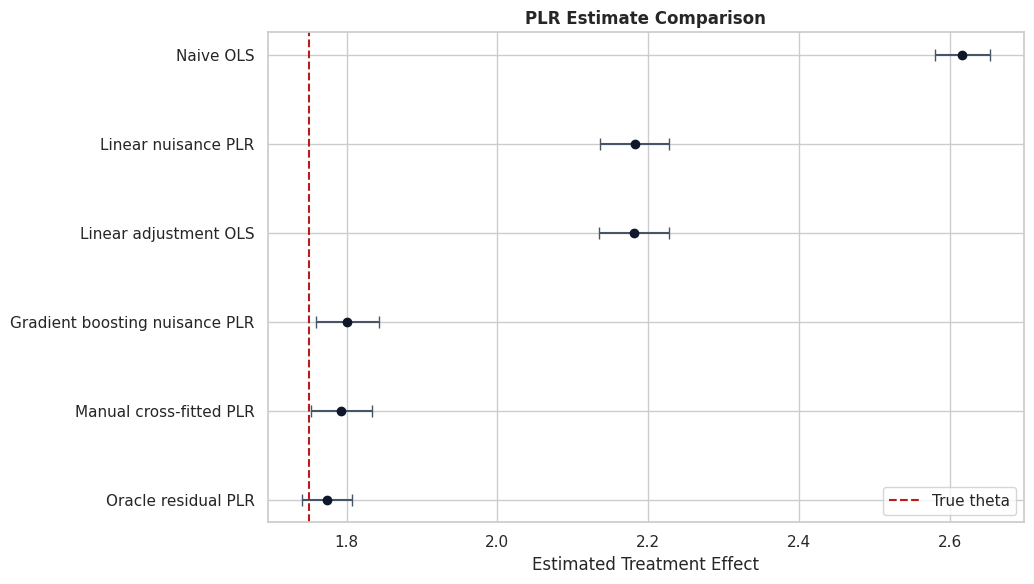
Baseline Estimate Plot
The next plot turns the baseline table into a compact visual check. The dashed vertical line is the true treatment effect used in the simulation.
This kind of comparison is helpful in teaching settings. In real applications, replace the true-effect line with design-based sensitivity checks and transparent uncertainty reporting.
The plot makes the main motivation visible. A treatment-effect workflow should not stop at a raw slope. We need an estimator that uses flexible nuisance functions while preserving valid treatment-effect inference.
Nuisance Learners For PLR
PLR needs two predictive models:
ml_l: predicts the outcome from controls, l(X) = E[Y | X].
ml_m: predicts the treatment from controls, m(X) = E[D | X].
The learners should be good enough to capture important confounding structure, but they are not the final object of interest. The final object is the orthogonal treatment-effect estimate.
We will use two learner families:
a regularized linear model, useful as a transparent baseline;
histogram gradient boosting, useful for nonlinear nuisance functions.
linear_nuisance = make_pipeline( StandardScaler(), LassoCV(cv=3, random_state=RANDOM_STATE, max_iter=5_000),)gradient_boosting_nuisance = HistGradientBoostingRegressor( max_iter=220, learning_rate=0.05, max_leaf_nodes=24, l2_regularization=0.001, random_state=RANDOM_STATE,)learner_catalog = pd.DataFrame( [ {"learner_name": "Regularized linear nuisance","sklearn_object": type(linear_nuisance).__name__,"why_use_it": "Transparent baseline; fast; may underfit nonlinear nuisance functions.", }, {"learner_name": "Histogram gradient boosting nuisance","sklearn_object": type(gradient_boosting_nuisance).__name__,"why_use_it": "Captures nonlinearities and interactions in this synthetic assignment rule.", }, ])save_table(learner_catalog, "learner_catalog")display(learner_catalog)
learner_name
sklearn_object
why_use_it
0
Regularized linear nuisance
Pipeline
Transparent baseline; fast; may underfit nonli...
1
Histogram gradient boosting nuisance
HistGradientBoostingRegressor
Captures nonlinearities and interactions in th...
The learner choice is part of the analysis, not a decoration. If both outcome and treatment nuisance models underfit the assignment structure, the orthogonal score has less to work with.
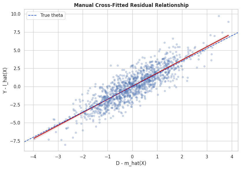
Manual Cross-Fitted Residualization
Before using DoubleML, we manually compute the partialling-out estimate with cross-fitted nuisance predictions.
The key rule is that each row’s nuisance prediction should come from a model that did not train on that row. This is the purpose of cross-fitting. It avoids using overly optimistic in-sample predictions inside the score.
The steps are:
Split the data into folds.
Predict Y from X out of fold.
Predict D from X out of fold.
Compute residuals.
Regress residualized Y on residualized D using the orthogonal score formula.
This cell is the core PLR idea in plain Python. DoubleML automates the same logic, adds carefully implemented variance calculations, repeated sample splitting, multiple treatment support, bootstrap tools, and a consistent API.
Check The Manual Nuisance Predictions
Because this is synthetic data, we can compare predicted nuisances to the true nuisance functions. This is a teaching privilege, not something we usually get in practice.
For real data, the corresponding diagnostics would use out-of-fold RMSE, residual plots, and domain checks rather than true nuisance comparisons.
The nuisance models do not need to be perfect. The point of orthogonality is that small nuisance errors should have limited first-order effect on the final estimate. Still, poor nuisance quality can increase bias, variance, and instability.
Manual Residual Plot
The residual plot shows the final identifying variation used by PLR. After removing the part of treatment and outcome explained by X, the slope of residualized outcome on residualized treatment estimates theta.
This is one of the most useful plots for explaining PLR to a stakeholder: it separates the raw treatment-outcome association from the residual treatment variation that remains after adjustment.
The residual cloud is centered near zero because both variables have been partialled out with respect to controls. The estimated slope is now much closer to the causal slope than the raw regression slope.
Build The DoubleML Data Object
DoubleMLData stores the roles that define the estimation problem:
y_col: outcome column.
d_cols: treatment column or columns.
x_cols: observed controls.
The hidden teaching columns are intentionally excluded from x_cols. In real analysis, including post-treatment, outcome-derived, or target-leaking columns is one of the fastest ways to create a polished but invalid estimate.
This object is where the estimand becomes concrete. If the role assignment is wrong, the estimator can run perfectly and still answer the wrong question.
Fit DoubleMLPLR With Flexible Nuisance Models
We now fit two DoubleML PLR models:
one with regularized linear nuisance learners;
one with gradient-boosted nuisance learners.
Both use the partialling-out score and five-fold cross-fitting. The treatment-effect estimate is still a single slope, but the nuisance functions can be nonlinear.
Finished: Linear nuisance PLR
Finished: Gradient boosting nuisance PLR
estimator
treatment
theta_hat
std_error
t_stat
p_value
ci_95_lower
ci_95_upper
true_theta
bias_vs_truth
0
Linear nuisance PLR
exposure_intensity
2.181998
0.023493
92.877976
0.0
2.135953
2.228044
1.75
0.431998
1
Gradient boosting nuisance PLR
exposure_intensity
1.801226
0.021146
85.179748
0.0
1.759780
1.842672
1.75
0.051226
The gradient-boosted nuisance model is expected to perform better here because the simulated assignment and outcome nuisance functions are nonlinear. The linear nuisance model remains useful because it shows how underfitting nuisance functions can move the final effect estimate.
Compare All Estimators
This table joins the simple baselines, manual cross-fitted PLR, and DoubleML estimates.
A useful habit is to compare estimators by what variation they use, not just by which package produced them. Naive OLS uses raw treatment variation. PLR uses treatment variation left after adjustment for observed controls.
The comparison shows the intended lesson: flexible residualization can move the estimate toward the true causal slope, while naive and underfit approaches can retain confounding bias.
Estimate Comparison Plot
The figure below summarizes the estimator comparison with confidence intervals. The red dashed line marks the true effect used in the simulation.
For a real dataset, the same plot is still useful, but the reference line would usually be absent. The emphasis would be on how estimates change across credible specifications.
The plot is also a communication tool. It shows why the modeling choice is not cosmetic: nuisance quality changes the final causal estimate.
DoubleML Nuisance Losses
evaluate_learners() reports out-of-fold RMSE for the nuisance learners. For PLR, the two learner keys are:
ml_l: outcome nuisance learner;
ml_m: treatment nuisance learner.
Lower nuisance RMSE is generally helpful, but the treatment-effect estimate is not chosen by nuisance RMSE alone. A learner can predict well while still producing unstable residual variation or violating design assumptions.
loss_tables = []for model_name, model in plr_models.items(): loss_tables.append(learner_loss_table(model, model_name))nuisance_losses = pd.concat(loss_tables, ignore_index=True)save_table(nuisance_losses, "doubleml_nuisance_losses")display(nuisance_losses)
model
learner
mean_rmse
min_rmse
max_rmse
0
Linear nuisance PLR
ml_l
2.975556
2.975556
2.975556
1
Linear nuisance PLR
ml_m
1.216985
1.216985
1.216985
2
Gradient boosting nuisance PLR
ml_l
2.327297
2.327297
2.327297
3
Gradient boosting nuisance PLR
ml_m
1.114093
1.114093
1.114093
The loss table helps explain why the gradient-boosting specification is more credible in this synthetic design. It is better matched to the nonlinear treatment assignment and outcome nuisance functions.
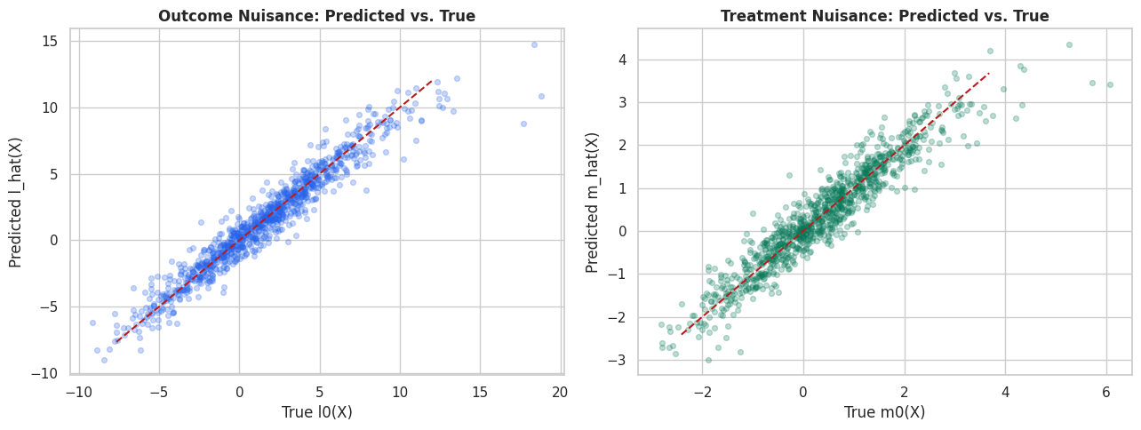
Nuisance Predictions Against Truth
Because this is a simulation, we can directly compare DoubleML’s out-of-fold nuisance predictions to the true nuisance functions.
This cell extracts the stored predictions from the gradient-boosted DoubleML model and computes RMSE, MAE, correlation, and observed-target R-squared.
The nuisance predictions are far from perfect, but they capture enough of the assignment and outcome structure to reduce the confounding bias substantially.
Visual Nuisance Diagnostics
The next figure compares predicted nuisance functions against the true nuisance functions. Again, this is possible only because the data are synthetic.
The important practical habit is the same for real data: inspect nuisance behavior instead of treating the effect estimate as a black box.
The treatment nuisance is often especially important in PLR because residualized treatment variation forms the denominator of the score. If m_hat(X) leaves systematic assignment patterns in the residual, the final slope can remain biased.
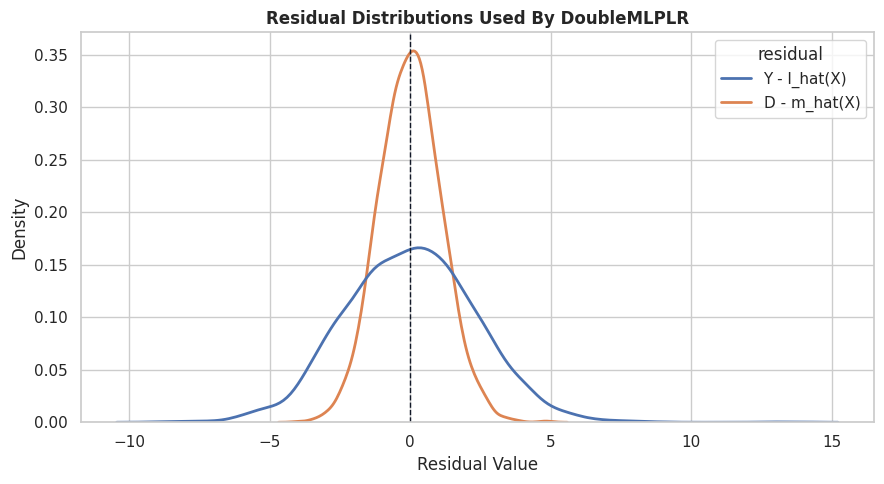
Residual Distribution Diagnostics
The residuals used by DoubleML should have meaningful spread. If the treatment residual is nearly zero for most units, then the design has weak residual treatment variation after controlling for X.
This cell compares the residualized treatment and outcome distributions from the gradient-boosting DoubleML fit.
The residualized treatment has enough spread to estimate a slope. If it collapsed near zero, the analysis would be warning us that the observed controls nearly determine treatment, leaving little quasi-experimental variation.
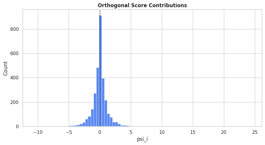
Orthogonal Score Values
DoubleML stores the score contributions psi. Large or highly skewed score contributions can signal instability, influential rows, or a need for more careful diagnostics.
Here we summarize and plot the score contributions from the gradient-boosted PLR fit.
The score is centered near zero at the fitted estimate, which is exactly what the estimating equation requires. The tails remind us that a small set of observations can still matter for uncertainty.
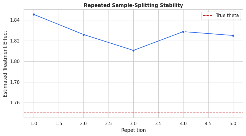
Repeated Sample Splitting
The estimate can vary slightly depending on how folds are drawn. Repeated sample splitting reruns the cross-fitting procedure under multiple splits and aggregates the result.
This cell uses a lighter gradient-boosting learner so the repeated-split check stays fast. The goal is not to tune the best learner; it is to see whether the estimate is stable across split draws.
Small movement across repetitions is normal. Large movement would suggest unstable nuisance learning, weak residual treatment variation, or a need for more observations, different learners, or a sharper design.
Split Stability Plot
The next figure shows the repeated-split estimates with the true effect as a reference line. It is a quick visual check for fold sensitivity.
This stability check is a lightweight guardrail. It does not validate identification, but it helps detect whether the numerical estimate is fragile to the random fold split.
Bootstrap Confidence Interval
DoubleML can compute bootstrap-based inference. For a single treatment, the ordinary confidence interval and bootstrap interval are often similar, but bootstrap tools become especially useful for joint inference and multiple parameters.
We run a moderate bootstrap here to keep the tutorial fast.
The bootstrap interval is another uncertainty summary around the same identifying design. It does not address omitted variables or bad controls; it quantifies sampling uncertainty conditional on the model and assumptions.
A Small Sensitivity Check
PLR still relies on observed-control identification. If important unobserved variables affect both treatment and outcome, the estimate can be biased.
DoubleML includes sensitivity tools for supported models. We run a small illustrative sensitivity scenario here and save the text summary. A later notebook in this tutorial series will go deeper into sensitivity analysis.
The sensitivity output should be read as a robustness exercise, not as proof that unobserved confounding is absent. It asks how strong omitted-confounder relationships would need to be under the chosen scenario.
When PLR Is The Wrong Tool
PLR is powerful, but it is not universal.
Use a different design when:
The treatment is binary and the target is ATE or ATT: consider DoubleMLIRM.
The treatment is endogenous even after observed controls: consider an IV design such as DoubleMLPLIV if a credible instrument exists.
The effect is expected to vary strongly across groups: combine PLR with heterogeneity tools or move to a model that targets CATE/GATE/BLP explicitly.
The data are panel, event-time, sample-selection, or discontinuity data: use the corresponding design rather than forcing a PLR setup.
The available controls include post-treatment variables: redesign the feature set before estimating.
The estimator should follow the causal question. Do not choose PLR just because it is convenient.
Reporting Checklist
This checklist turns the notebook into a reusable applied workflow. A credible PLR report should describe not only the estimate but also the design, role assignment, nuisance models, uncertainty, and limitations.
reporting_checklist = pd.DataFrame( [ {"item": "Causal question", "status": "Stated as effect of exposure_intensity on weekly_value."}, {"item": "Treatment type", "status": "Continuous dose; PLR is appropriate for a constant-slope estimand."}, {"item": "Control timing", "status": "All controls are pre-treatment by construction in this synthetic dataset."}, {"item": "Nuisance learners", "status": "Compared regularized linear and gradient-boosted nuisance models."}, {"item": "Cross-fitting", "status": "Used five folds; manually demonstrated residualization and used DoubleMLPLR."}, {"item": "Uncertainty", "status": "Reported standard errors, confidence intervals, and a bootstrap interval."}, {"item": "Stability", "status": "Checked repeated sample splitting."}, {"item": "Sensitivity", "status": "Ran a small illustrative unobserved-confounding sensitivity scenario."}, {"item": "Main limitation", "status": "Synthetic truth is known here; real use requires defensible observed-control identification."}, ])save_table(reporting_checklist, "plr_reporting_checklist")display(reporting_checklist)
item
status
0
Causal question
Stated as effect of exposure_intensity on week...
1
Treatment type
Continuous dose; PLR is appropriate for a cons...
2
Control timing
All controls are pre-treatment by construction...
3
Nuisance learners
Compared regularized linear and gradient-boost...
4
Cross-fitting
Used five folds; manually demonstrated residua...
5
Uncertainty
Reported standard errors, confidence intervals...
6
Stability
Checked repeated sample splitting.
7
Sensitivity
Ran a small illustrative unobserved-confoundin...
8
Main limitation
Synthetic truth is known here; real use requir...
The checklist is deliberately plain. Good causal reporting is often about making assumptions and diagnostics visible, not about adding more model complexity.
Report Template
The next cell writes a short markdown report template using the main estimate from the gradient-boosted PLR model. This can be adapted for real analyses by replacing the synthetic-data checks with design-specific evidence.
main_row = plr_summary.loc[plr_summary["estimator"] =="Gradient boosting nuisance PLR"].iloc[0]report_text =f"""# PLR Effect Estimate Report Template## Causal QuestionEstimate the constant-slope effect of `exposure_intensity` on `weekly_value`, adjusting for pre-treatment controls.## EstimatorThe main estimator is `DoubleMLPLR` with the partialling-out score, five-fold cross-fitting, and histogram gradient-boosting nuisance learners for `ml_l` and `ml_m`.## Main Estimate- Estimated effect: {main_row['theta_hat']:.4f}- Standard error: {main_row['std_error']:.4f}- 95 percent confidence interval: [{main_row['ci_95_lower']:.4f}, {main_row['ci_95_upper']:.4f}]## Diagnostics Included- Baseline comparisons against naive and linearly adjusted OLS.- Manual cross-fitted residualization.- Nuisance learner RMSE checks.- Residual distribution checks.- Orthogonal score contribution checks.- Repeated sample-splitting stability.- Bootstrap confidence interval.- Small illustrative sensitivity analysis.## Required AssumptionsThe PLR estimate relies on observed-control identification: after adjusting for the selected pre-treatment controls, residual treatment variation is as-good-as-random for the outcome. The model does not solve omitted confounding or bad-control problems by itself.""".strip()report_path = REPORT_DIR /f"{NOTEBOOK_PREFIX}_plr_report_template.md"report_path.write_text(report_text)print(report_text)
# PLR Effect Estimate Report Template

## Causal Question
Estimate the constant-slope effect of `exposure_intensity` on `weekly_value`, adjusting for pre-treatment controls.

## Estimator
The main estimator is `DoubleMLPLR` with the partialling-out score, five-fold cross-fitting, and histogram gradient-boosting nuisance learners for `ml_l` and `ml_m`.

## Main Estimate
- Estimated effect: 1.8012
- Standard error: 0.0211
- 95 percent confidence interval: [1.7598, 1.8427]

## Diagnostics Included
- Baseline comparisons against naive and linearly adjusted OLS.
- Manual cross-fitted residualization.
- Nuisance learner RMSE checks.
- Residual distribution checks.
- Orthogonal score contribution checks.
- Repeated sample-splitting stability.
- Bootstrap confidence interval.
- Small illustrative sensitivity analysis.

## Required Assumptions
The PLR estimate relies on observed-control identification: after adjusting for the selected pre-treatment controls, residual treatment variation is as-good-as-random for the outcome. The model does not solve omitted confounding or bad-control problems by itself.
This report template keeps the estimate attached to its assumptions. That is the right posture for DoubleML: the package helps estimate a design-based target, but the design itself still has to be argued.
Artifact Manifest
The final cell lists the artifacts produced by this notebook. This makes it easier to find saved tables, figures, datasets, and reports later.
The PLR notebook is now complete. The next natural topic is the partially linear instrumental-variable model, where the treatment may still be endogenous after observed controls and a credible instrument is needed.