DoubleML Tutorial 02: Data Backend, DoubleMLData, And Design Setup
This notebook is about the part of DoubleML that looks simple but carries a lot of causal responsibility: the data backend. Before fitting a model, DoubleML needs to know which column is the outcome, which column is the treatment, which columns are controls, which columns are instruments, which columns define clusters or panels, and which columns are design-specific variables such as running scores or selection indicators.
The data backend is not just a convenience wrapper. It is where the causal design becomes an executable object. If the column roles are wrong, the estimand is wrong. If a post-treatment variable is placed in the controls, the nuisance model can adjust away part of the effect. If an instrument is accidentally treated as an ordinary control, the IV design is no longer represented. If clustered observations are treated as independent, uncertainty can be overstated.
This tutorial therefore focuses on design setup, schema checks, and backend construction before model fitting. The actual estimators come in later notebooks.
Estimated runtime: less than 1 minute.
Learning Goals
By the end of this notebook, you should be able to:
explain why variable roles define the causal estimand;
build DoubleMLData objects for standard, IV, multi-treatment, and clustered designs;
understand when DoubleMLPanelData, DoubleMLRDDData, and DoubleMLSSMData are relevant;
create a repeatable data audit before fitting any DoubleML model;
detect common setup mistakes such as missing values, overlapping roles, post-treatment controls, and weak treatment variation;
save a data-design report that can be reused before model fitting.
Tutorial Flow
The notebook follows a practical workflow:
define the theory of data roles and estimands;
create a synthetic master dataset with many possible design columns;
audit missingness, numeric types, variation, correlations, and role conflicts;
construct standard DoubleMLData objects;
construct IV, multi-treatment, clustered, panel, RDD, and sample-selection backends;
show common mistakes and how to catch them early;
finish with a reusable design checklist and artifact manifest.
Setup
This cell imports the scientific Python stack, configures output folders, and imports DoubleML. We suppress known non-substantive notebook warnings so the executed notebook stays readable.
from pathlib import Pathimport inspectimport osimport warningsPROJECT_ROOT = Path.cwd().resolve()if PROJECT_ROOT.name =="doubleml": PROJECT_ROOT = PROJECT_ROOT.parents[2]OUTPUT_DIR = PROJECT_ROOT /"notebooks"/"tutorials"/"doubleml"/"outputs"DATASET_DIR = OUTPUT_DIR /"datasets"FIGURE_DIR = OUTPUT_DIR /"figures"TABLE_DIR = OUTPUT_DIR /"tables"REPORT_DIR = OUTPUT_DIR /"reports"MATPLOTLIB_CACHE_DIR = OUTPUT_DIR /"matplotlib_cache"for directory in [DATASET_DIR, FIGURE_DIR, TABLE_DIR, REPORT_DIR, MATPLOTLIB_CACHE_DIR]: directory.mkdir(parents=True, exist_ok=True)os.environ.setdefault("MPLCONFIGDIR", str(MATPLOTLIB_CACHE_DIR))warnings.filterwarnings("ignore", category=FutureWarning)warnings.filterwarnings("ignore", message="IProgress not found.*")warnings.filterwarnings("ignore", message=".*does not have valid feature names.*")warnings.filterwarnings("ignore", message="DoubleMLDIDData is deprecated.*")import numpy as npimport pandas as pdimport matplotlib.pyplot as pltimport seaborn as snsfrom IPython.display import displayimport doubleml as dmlNOTEBOOK_PREFIX ="02"RANDOM_SEED =42sns.set_theme(style="whitegrid", context="notebook")plt.rcParams.update({"figure.dpi": 120, "savefig.dpi": 160})print(f"Project root: {PROJECT_ROOT}")print(f"Output folder: {OUTPUT_DIR}")print(f"DoubleML version: {getattr(dml, '__version__', 'not exposed')}")
The setup mirrors the earlier notebooks so outputs are organized consistently. All generated files in this notebook use the 02_ prefix.
Package Versions
Backend behavior and constructor signatures can change across versions, so we record the environment used for this run.
from importlib import metadatapackages = ["doubleml", "numpy", "pandas", "scikit-learn", "matplotlib", "seaborn"]version_rows = []for package in packages:try: version = metadata.version(package)except metadata.PackageNotFoundError: version =None version_rows.append({"package": package, "version": version})version_table = pd.DataFrame(version_rows)version_table.to_csv(TABLE_DIR /f"{NOTEBOOK_PREFIX}_package_versions.csv", index=False)display(version_table)
package
version
0
doubleml
0.11.2
1
numpy
2.4.4
2
pandas
3.0.2
3
scikit-learn
1.6.1
4
matplotlib
3.10.9
5
seaborn
0.13.2
This table is especially useful for a backend tutorial because class names and preferred containers can evolve over time.
Theory: Data Roles Define The Estimand
A DoubleML estimator does not discover the role of each column. You tell it the roles. That role assignment defines which score is evaluated and which nuisance functions are estimated.
For a standard unconfoundedness design, a simplified role map is:
Y: the outcome we want to explain causally;
D: the treatment or exposure whose effect is targeted;
X: pre-treatment controls used to make treatment assignment as-good-as-random conditional on X;
optional clusters: groups that affect dependence in the data;
optional instruments Z: variables that shift treatment but affect the outcome only through treatment under IV assumptions.
For other designs, the backend may also need:
t_col: a time column for panel or DID-style data;
id_col: a unit identifier for panel data;
score_col: the running variable in an RDD setup;
s_col: a selection indicator for sample-selection models.
The central rule is: if a column’s role is conceptually wrong, a successful Python object can still encode a bad causal design.
The following table turns this theory into a role glossary. This is the checklist to keep beside every DoubleML data object.
role_glossary = pd.DataFrame( [ {"role": "outcome","typical_argument": "y_col","causal_meaning": "Final outcome whose causal response is being studied.","common_mistake": "Using an intermediate or post-treatment measure as the outcome by accident.", }, {"role": "treatment","typical_argument": "d_cols","causal_meaning": "Exposure, policy, product change, or intervention variable whose effect is targeted.","common_mistake": "Mixing multiple treatments without deciding whether the estimand is joint or separate.", }, {"role": "controls","typical_argument": "x_cols","causal_meaning": "Pre-treatment adjustment variables used by nuisance learners.","common_mistake": "Including post-treatment mediators or colliders as controls.", }, {"role": "instruments","typical_argument": "z_cols","causal_meaning": "Variables that shift treatment but are excluded from the outcome equation except through treatment.","common_mistake": "Treating an instrument like an ordinary confounder or using a weak instrument.", }, {"role": "clusters","typical_argument": "cluster_cols","causal_meaning": "Group identifiers for dependence across rows.","common_mistake": "Ignoring repeated users, markets, schools, stores, or sessions as independent rows.", }, {"role": "time and unit identifiers","typical_argument": "t_col, id_col","causal_meaning": "Panel structure for repeated observations over time.","common_mistake": "Using row order instead of explicit time and unit columns.", }, {"role": "running score","typical_argument": "score_col","causal_meaning": "RDD assignment variable around a cutoff.","common_mistake": "Using a transformed treatment indicator instead of the underlying running variable.", }, {"role": "selection indicator","typical_argument": "s_col","causal_meaning": "Indicator for whether the outcome is observed or the row is selected into the analytic sample.","common_mistake": "Dropping unselected rows before modeling selection.", }, ])role_glossary.to_csv(TABLE_DIR /f"{NOTEBOOK_PREFIX}_role_glossary.csv", index=False)display(role_glossary)
role
typical_argument
causal_meaning
common_mistake
0
outcome
y_col
Final outcome whose causal response is being s...
Using an intermediate or post-treatment measur...
1
treatment
d_cols
Exposure, policy, product change, or intervent...
Mixing multiple treatments without deciding wh...
2
controls
x_cols
Pre-treatment adjustment variables used by nui...
Including post-treatment mediators or collider...
3
instruments
z_cols
Variables that shift treatment but are exclude...
Treating an instrument like an ordinary confou...
4
clusters
cluster_cols
Group identifiers for dependence across rows.
Ignoring repeated users, markets, schools, sto...
5
time and unit identifiers
t_col, id_col
Panel structure for repeated observations over...
Using row order instead of explicit time and u...
6
running score
score_col
RDD assignment variable around a cutoff.
Using a transformed treatment indicator instea...
7
selection indicator
s_col
Indicator for whether the outcome is observed ...
Dropping unselected rows before modeling selec...
The glossary should feel conservative. Most DoubleML mistakes are not exotic math failures; they are role-assignment mistakes made before the estimator starts.
Installed Data Containers
The next cell inspects the data-container classes available in the installed DoubleML version. This makes the notebook version-aware and shows which constructor arguments matter.
container_names = ["DoubleMLData","DoubleMLClusterData","DoubleMLPanelData","DoubleMLDIDData","DoubleMLRDDData","DoubleMLSSMData",]container_rows = []for name in container_names: cls =getattr(dml, name, None)if cls isNone: container_rows.append({"container": name, "available": False, "signature": None, "note": "not available"})continue doc = inspect.getdoc(cls) or"" first_doc_line = doc.splitlines()[0] if doc else"" note ="available"if"deprecated"in doc.lower(): note ="available but not preferred in this version" container_rows.append( {"container": name,"available": True,"signature": str(inspect.signature(cls)),"note": note,"doc_summary": first_doc_line, } )container_table = pd.DataFrame(container_rows)container_table.to_csv(TABLE_DIR /f"{NOTEBOOK_PREFIX}_container_signatures.csv", index=False)display(container_table)
container
available
signature
note
doc_summary
0
DoubleMLData
True
(data, y_col, d_cols, x_cols=None, z_cols=None...
available
Double machine learning data-backend.
1
DoubleMLClusterData
True
(data, y_col, d_cols, cluster_cols, x_cols=Non...
available but not preferred in this version
Backwards compatibility wrapper for DoubleMLDa...
2
DoubleMLPanelData
True
(data, y_col, d_cols, t_col, id_col, x_cols=No...
available
Double machine learning data-backend for panel...
3
DoubleMLDIDData
True
(data, y_col, d_cols, x_cols=None, z_cols=None...
available
Double machine learning data-backend for Diffe...
4
DoubleMLRDDData
True
(data, y_col, d_cols, score_col, x_cols=None, ...
available
Double machine learning data-backend for Regre...
5
DoubleMLSSMData
True
(data, y_col, d_cols, x_cols=None, z_cols=None...
available
Double machine learning data-backend for Sampl...
The preferred starting point is DoubleMLData. Specialized containers become useful when the design itself needs extra structure, such as unit-time panels, RDD running scores, or sample-selection indicators.
Create A Master Teaching Dataset
We now create one synthetic master dataset containing columns for several possible designs. Not every column belongs in every design. That is deliberate: a realistic data table often contains outcomes, treatments, controls, instruments, identifiers, timestamps, post-treatment variables, and helper columns all at once.
The point of the backend workflow is to choose the correct subset and assign roles carefully.
The master table contains more columns than any single design should use. The next sections will carve it into different DoubleML backend objects.
Variable Dictionary
A variable dictionary is the first line of defense against role confusion. We mark each column’s conceptual role and whether it is safe to use as a pre-treatment control in standard effect-estimation designs.
The row for post_treatment_engagement is especially important. It is predictive of the outcome, but it is not a valid standard control if the target is the effect of treatment on outcome.
Basic Data Audit
A backend object can be created only when the data satisfies practical requirements: finite values, variation in treatment, expected data types, and no accidental missingness. This audit is intentionally generic so it can be reused before any DoubleML model.
The audit shows no missingness and enough variation in the treatment columns. It also reminds us that identifier columns are numeric, which means they could accidentally slip into controls if we select columns mechanically.
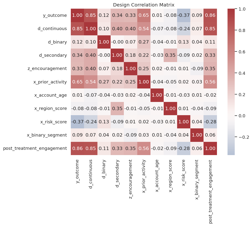
Correlation And Design Pressure
Correlation is not a causal design, but it is a useful diagnostic. Here we inspect treatment, outcome, instrument, and control associations to understand the structure of the teaching data.
The post-treatment variable is highly related to the outcome and treatment, which is exactly why it is tempting and dangerous as a control. The instrument is related to the continuous treatment, which is useful for IV examples but still requires exclusion assumptions in real applications.
Backend Helper Functions
The next helper functions summarize DoubleML data objects in tables. This makes the output easy to compare across standard, IV, cluster, panel, RDD, and sample-selection designs.
The overlap helper catches one of the most common setup errors: the same column being assigned as both treatment and control, or as both instrument and control.
Standard DoubleMLData For PLR
The standard cross-sectional backend uses DoubleMLData. We start with a continuous-treatment design suitable for PLR-style estimators.
The printed object should show one outcome, one treatment, five covariates, no instruments, and the full row count. This confirms the standard PLR-ready backend.
Now we save a compact backend summary. This is useful when comparing many design objects in one notebook.
backend_summaries = [ summarize_backend("standard_plr_continuous_treatment", plr_backend,"Continuous treatment with pre-treatment controls for PLR-style estimators.", )]backend_summary_table = pd.DataFrame(backend_summaries)backend_summary_table.to_csv(TABLE_DIR /f"{NOTEBOOK_PREFIX}_backend_summary_initial.csv", index=False)display(backend_summary_table)
backend_name
backend_class
outcome
treatments
controls
instruments
clusters
time_col
id_col
score_col
selection_col
n_obs
design_note
0
standard_plr_continuous_treatment
DoubleMLData
y_outcome
d_continuous
x_prior_activity, x_account_age, x_region_scor...
None
None
None
None
900
Continuous treatment with pre-treatment contro...
The first backend is deliberately simple. The later backend objects add one design feature at a time.
Binary-Treatment Backend For IRM
For binary-treatment models such as IRM, the backend still uses DoubleMLData. The difference is conceptual: d_cols now points to a binary treatment, and later model classes will use propensity-score-style nuisance functions.
The treated and control shares are both comfortably away from zero. That does not prove overlap, but it catches the extreme failure where one group is nearly absent.
Instrumental-Variable Backend
An IV setup adds z_cols. The instrument must be assigned explicitly; otherwise the backend will treat the design as non-IV. The package cannot verify the exclusion restriction for us, but the data object can represent the intended instrument role.
The instrument is related to the treatment in this synthetic data. In real IV work, relevance is only one requirement; exclusion and independence are design assumptions that need separate evidence.
Multi-Treatment Backend
DoubleMLData can hold multiple treatments. The argument use_other_treat_as_covariate controls whether other treatment variables are automatically included as controls when one treatment is targeted.
This is a subtle modeling choice. If treatments are jointly assigned, using the other treatment as a covariate changes the estimand from a total effect toward a partial effect holding the other treatment fixed.
multi_treatment_backend = dml.DoubleMLData( master_df, y_col="y_outcome", d_cols=["d_continuous", "d_secondary"], x_cols=standard_x_cols, use_other_treat_as_covariate=True,)multi_treatment_backend_no_auto = dml.DoubleMLData( master_df, y_col="y_outcome", d_cols=["d_continuous", "d_secondary"], x_cols=standard_x_cols, use_other_treat_as_covariate=False,)multi_treatment_policy = pd.DataFrame( [ {"backend": "use_other_treat_as_covariate_true","use_other_treat_as_covariate": True,"design_meaning": "Estimate each treatment effect while treating the other treatment as an additional adjustment variable.", }, {"backend": "use_other_treat_as_covariate_false","use_other_treat_as_covariate": False,"design_meaning": "Do not automatically adjust for the other treatment; use when the estimand is defined that way.", }, ])multi_treatment_policy.to_csv(TABLE_DIR /f"{NOTEBOOK_PREFIX}_multi_treatment_policy.csv", index=False)display(multi_treatment_policy)print(multi_treatment_backend)
The object prints both treatments. The policy table is the important part: multi-treatment designs need an estimand decision before fitting.
Clustered Backend
Cluster columns represent dependence across rows. Examples include repeated users, schools, stores, geographies, or sessions. In this installed version, cluster columns can be supplied directly to DoubleMLData, which is the preferred modern pattern.
The cluster audit shows enough groups and rows per group for a teaching example. In real work, very few clusters or highly unbalanced clusters should be flagged before inference.
Panel Backend
Panel data has repeated observations for units over time. The DoubleMLPanelData backend requires both a time column and a unit identifier. We create a compact long-format panel dataset from scratch so the structure is obvious.
The panel backend records the unit and time roles explicitly. This is safer than relying on row order or dataframe sorting.
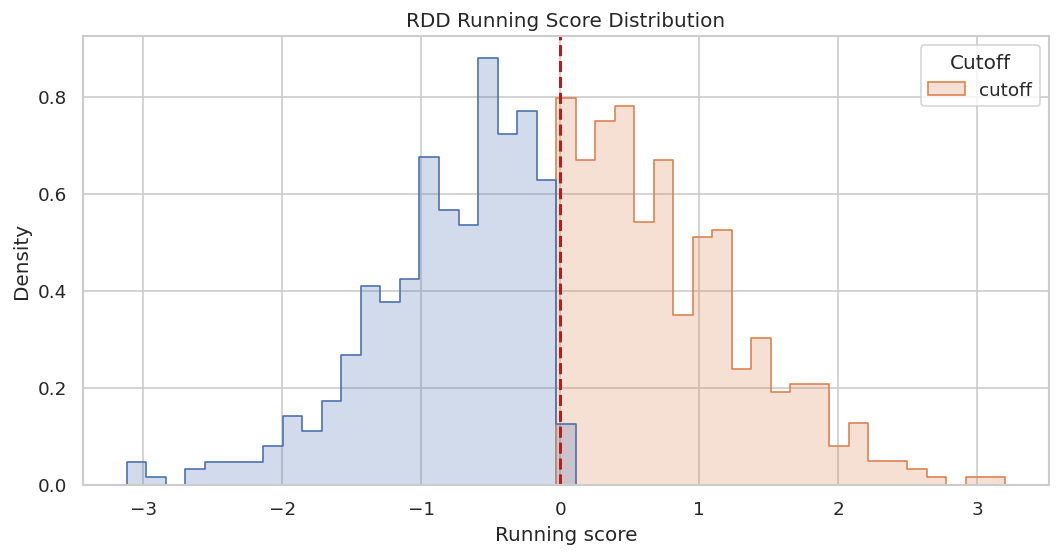
RDD Backend
Regression discontinuity designs require a running score and a treatment assignment around a cutoff. DoubleMLRDDData records the running score through score_col. The treatment indicator is still supplied through d_cols.
The RDD audit checks local support around the cutoff. A running score with no observations near the cutoff would be a design problem before any model fitting.
The next figure shows the running score distribution and the cutoff. It is a quick visual check that the data has observations on both sides.
The distribution has support on both sides of zero. Later RDD modeling will need stronger checks, but this is the right backend-level starting point.
Sample-Selection Backend
Sample-selection models use a selection indicator, supplied as s_col. The key idea is that outcome observation or analytic inclusion may not be random. The backend needs the selection column so the model can represent that design.
The selected share is neither zero nor one, so the selection indicator has variation. That is the first minimal requirement for a sample-selection design.
Combined Backend Summary
Now we collect all constructed backend objects into one table. This table gives a compact view of how the same master data can support different designs when roles are assigned differently.
backend_objects = [ ("standard_plr_continuous_treatment", plr_backend, "Continuous treatment with pre-treatment controls."), ("standard_irm_binary_treatment", irm_backend, "Binary treatment with pre-treatment controls."), ("iv_pliv_continuous_treatment", iv_backend, "Continuous treatment plus instrument."), ("multi_treatment", multi_treatment_backend, "Two treatment columns with other treatment used as covariate."), ("clustered_plr", cluster_backend, "Continuous treatment with cluster identifier."), ("panel_long_format", panel_backend, "Repeated unit-time observations."), ("rdd_running_score", rdd_backend, "RDD score and cutoff treatment."), ("sample_selection", selection_backend, "Selection indicator supplied."),]backend_summary_table = pd.DataFrame([summarize_backend(*item) for item in backend_objects])backend_summary_table.to_csv(TABLE_DIR /f"{NOTEBOOK_PREFIX}_backend_summary_table.csv", index=False)display(backend_summary_table)
backend_name
backend_class
outcome
treatments
controls
instruments
clusters
time_col
id_col
score_col
selection_col
n_obs
design_note
0
standard_plr_continuous_treatment
DoubleMLData
y_outcome
d_continuous
x_prior_activity, x_account_age, x_region_scor...
NaN
NaN
NaN
NaN
900
Continuous treatment with pre-treatment controls.
1
standard_irm_binary_treatment
DoubleMLData
y_outcome
d_binary
x_prior_activity, x_account_age, x_region_scor...
NaN
NaN
NaN
NaN
900
Binary treatment with pre-treatment controls.
2
iv_pliv_continuous_treatment
DoubleMLData
y_outcome
d_continuous
x_prior_activity, x_account_age, x_region_scor...
z_encouragement
NaN
NaN
NaN
NaN
900
Continuous treatment plus instrument.
3
multi_treatment
DoubleMLData
y_outcome
d_continuous, d_secondary
x_prior_activity, x_account_age, x_region_scor...
NaN
NaN
NaN
NaN
900
Two treatment columns with other treatment use...
4
clustered_plr
DoubleMLData
y_outcome
d_continuous
x_prior_activity, x_account_age, x_region_scor...
cluster_id
NaN
NaN
NaN
NaN
900
Continuous treatment with cluster identifier.
5
panel_long_format
DoubleMLPanelData
y_outcome
d_continuous
x_baseline, x_time_varying
time_period
unit_id
NaN
NaN
720
Repeated unit-time observations.
6
rdd_running_score
DoubleMLRDDData
y_outcome
d_rdd
x_prior_activity, x_account_age, x_region_scor...
NaN
NaN
running_score
NaN
900
RDD score and cutoff treatment.
7
sample_selection
DoubleMLSSMData
y_outcome
d_binary
x_prior_activity, x_account_age, x_region_scor...
NaN
NaN
NaN
selected
900
Selection indicator supplied.
This table is the core artifact of the notebook. It shows the role assignment that each later estimator would inherit.
Common Mistake: Overlapping Roles
DoubleML will often catch impossible role assignments, but it is better to catch them deliberately in your own audit. Here we create a mistaken role map that assigns d_continuous as both treatment and control.
The overlap audit catches the problem before model construction. This kind of check is worth automating in serious projects.
Common Mistake: Post-Treatment Controls
A post-treatment variable may be highly predictive of the outcome, but it is usually unsafe as a standard control for the total effect of treatment. This cell flags controls that are not allowed by the variable dictionary.
proposed_controls_with_bad_control = standard_x_cols + ["post_treatment_engagement"]allowed_lookup = variable_dictionary.set_index("column")["allowed_as_standard_control"].to_dict()post_treatment_control_check = pd.DataFrame( [ {"control": col,"allowed_as_standard_control": bool(allowed_lookup.get(col, False)),"role_family": variable_dictionary.set_index("column").loc[col, "role_family"] if col in allowed_lookup else"unknown", }for col in proposed_controls_with_bad_control ])post_treatment_control_check["problem"] =~post_treatment_control_check["allowed_as_standard_control"]post_treatment_control_check.to_csv(TABLE_DIR /f"{NOTEBOOK_PREFIX}_post_treatment_control_check.csv", index=False)display(post_treatment_control_check)
control
allowed_as_standard_control
role_family
problem
0
x_prior_activity
True
pre-treatment control
False
1
x_account_age
True
pre-treatment control
False
2
x_region_score
True
pre-treatment control
False
3
x_risk_score
True
pre-treatment control
False
4
x_binary_segment
True
pre-treatment control
False
5
post_treatment_engagement
False
post-treatment variable
True
The post-treatment variable is flagged. A backend object might still be constructible with that column, but the causal design would be different and usually not what we want for a total treatment effect.
Common Mistake: Missing Or Non-Finite Values
DoubleML backend constructors enforce finite controls by default. Here we intentionally create a missing value in one control column, catch the constructor error, and record the result as an audit table.
The constructor failure is helpful. It prevents silent fitting with an invalid design matrix. In applied work, decide on imputation or row exclusion before creating the backend object.
Common Mistake: Weak Treatment Variation
For binary-treatment designs, a backend can be created even if one group is tiny. That is a design warning because propensity and outcome nuisance models need support in both groups. This cell creates a reusable treatment-variation audit.
Both binary treatment examples have support in each group. This does not guarantee overlap conditional on controls, but it clears the first backend-level check.
Common Mistake: Mechanical Control Selection
A tempting shortcut is to define controls as every numeric column except outcome and treatment. That shortcut can accidentally include identifiers, instruments, post-treatment variables, running scores, and selection indicators.
This cell contrasts mechanical controls with approved controls from the variable dictionary.
mechanical_controls = [ col for col in master_df.select_dtypes(include=[np.number]).columnsif col notin ["y_outcome", "d_continuous"]]approved_controls = variable_dictionary.loc[variable_dictionary["allowed_as_standard_control"], "column"].tolist()mechanical_control_audit = pd.DataFrame( [ {"column": col,"selected_mechanically": col in mechanical_controls,"approved_standard_control": col in approved_controls,"role_family": variable_dictionary.set_index("column").loc[col, "role_family"],"problem_if_used_as_standard_control": (col in mechanical_controls) and (col notin approved_controls), }for col in mechanical_controls ])mechanical_control_audit.to_csv(TABLE_DIR /f"{NOTEBOOK_PREFIX}_mechanical_control_audit.csv", index=False)display(mechanical_control_audit)
column
selected_mechanically
approved_standard_control
role_family
problem_if_used_as_standard_control
0
user_id
True
False
identifier
True
1
cluster_id
True
False
cluster
True
2
time_period
True
False
time
True
3
d_binary
True
False
binary treatment
True
4
d_secondary
True
False
secondary treatment
True
5
z_encouragement
True
False
instrument
True
6
x_prior_activity
True
True
pre-treatment control
False
7
x_account_age
True
True
pre-treatment control
False
8
x_region_score
True
True
pre-treatment control
False
9
x_risk_score
True
True
pre-treatment control
False
10
x_binary_segment
True
True
pre-treatment control
False
11
post_treatment_engagement
True
False
post-treatment variable
True
12
running_score
True
False
RDD running score
True
13
d_rdd
True
False
RDD treatment
True
14
selected
True
False
selection indicator
True
The audit shows why column-selection shortcuts are dangerous. Numeric type is not the same thing as causal admissibility.
Design Readiness Matrix
This matrix summarizes which checks matter for each design family. It is a bridge from backend construction to model fitting in later notebooks.
This matrix is intentionally conservative. Passing a backend constructor is a starting point, not a complete design validation.
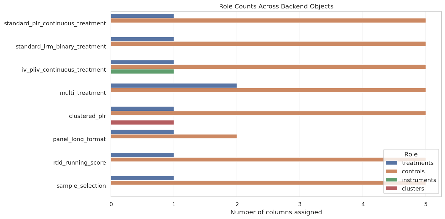
Visual Summary Of Backend Choices
The following plot counts how many columns are assigned to major roles in each backend object. It gives a quick visual overview of how role complexity changes across designs.
The plot shows that the same dataset supports different backend role structures. The backend should match the causal question, not the other way around.
Backend Construction Checklist
This checklist turns the notebook into a reusable pre-fit workflow. It should be completed before choosing nuisance learners or fitting a DoubleML estimator.
backend_checklist = pd.DataFrame( [ {"step": "State the estimand", "question": "What effect is targeted: continuous effect, ATE, IV effect, DID effect, RDD effect, or selection-adjusted effect?"}, {"step": "Define outcome", "question": "Is the outcome measured after treatment and aligned with the causal question?"}, {"step": "Define treatment", "question": "Is treatment continuous, binary, multi-valued, instrumented, or cutoff-assigned?"}, {"step": "Define controls", "question": "Are controls pre-treatment variables, not mediators, colliders, identifiers, or post-treatment consequences?"}, {"step": "Define instruments", "question": "If using IV, are instruments assigned through z_cols and backed by relevance/exclusion arguments?"}, {"step": "Define dependence structure", "question": "Are clusters, units, and time columns represented explicitly when rows are dependent?"}, {"step": "Audit missingness", "question": "Are all outcome, treatment, control, instrument, and design-specific columns finite or intentionally handled?"}, {"step": "Audit variation", "question": "Does treatment, instrument, running score, or selection indicator have enough support?"}, {"step": "Save backend summary", "question": "Can another analyst see exactly which columns were assigned to each role?"}, ])backend_checklist.to_csv(TABLE_DIR /f"{NOTEBOOK_PREFIX}_backend_construction_checklist.csv", index=False)display(backend_checklist)
step
question
0
State the estimand
What effect is targeted: continuous effect, AT...
1
Define outcome
Is the outcome measured after treatment and al...
2
Define treatment
Is treatment continuous, binary, multi-valued,...
3
Define controls
Are controls pre-treatment variables, not medi...
4
Define instruments
If using IV, are instruments assigned through ...
5
Define dependence structure
Are clusters, units, and time columns represen...
6
Audit missingness
Are all outcome, treatment, control, instrumen...
7
Audit variation
Does treatment, instrument, running score, or ...
8
Save backend summary
Can another analyst see exactly which columns ...
The checklist is the main habit to carry forward. A careful backend setup makes the estimator notebooks much easier and less error-prone.
Reusable Backend Report Template
The final report template is a short markdown file that can be filled before model fitting. It is intentionally focused on design and column roles.
backend_report_template ="""# DoubleML Backend Design Report## 1. Causal QuestionState the treatment, outcome, target population, and estimand.## 2. Backend ClassName the DoubleML backend class used and explain why it matches the design.## 3. Column Roles- Outcome column:- Treatment column(s):- Control columns:- Instrument column(s):- Cluster column(s):- Unit/time columns:- Running score column:- Selection column:## 4. Excluded ColumnsList columns intentionally excluded from controls, especially identifiers, instruments, post-treatment variables, colliders, mediators, and target leakage columns.## 5. Data AuditSummarize missingness, finite-value checks, data types, treatment variation, binary-treatment support, instrument support, cluster counts, panel balance, RDD cutoff support, or selection support as relevant.## 6. Assumption NotesState the identification assumptions that must be defended outside the backend object.## 7. Ready For Model Fitting?State what remains to check before fitting: nuisance learner choice, sample splitting, tuning, inference, and sensitivity."""report_path = REPORT_DIR /f"{NOTEBOOK_PREFIX}_backend_design_report_template.md"report_path.write_text(backend_report_template)print(report_path)
The template keeps the backend work visible. It is much easier to review a DoubleML analysis when the column roles are documented before model fitting begins.
Artifact Manifest
The final cell records all 02_* files created by the notebook.
The backend is where the causal design becomes machine-readable. The main lesson is simple: choose columns by causal role, not by convenience, data type, or predictive power.
The next notebook moves from backend setup into DoubleMLPLR, where we estimate continuous-treatment effects using the data roles introduced here.