causal-learn Tutorial 15: Benchmarking, Stability, And Sensitivity

A single causal discovery run is rarely enough. Discovery algorithms make assumptions about independence tests, scores, linearity, noise, hidden variables, sample size, and tuning choices. If a learned graph changes completely when one of those choices changes, the graph should be treated as a fragile hypothesis rather than a reliable structure.

This notebook builds a compact benchmarking workflow for causal-learn. We will simulate data from a known observed DAG, run several algorithm families, and then stress-test the learned graphs across sample size, noise, tuning settings, nonlinearity, and hidden confounding.

The goal is not to crown one universal best algorithm. The goal is to learn how to report causal discovery results honestly: what was stable, what changed, and which assumptions each method needed.

Estimated runtime: about 2-5 minutes. Most cells are fast; the repeated benchmark grids do several PC, GES, and DirectLiNGAM fits.

Learning Goals

By the end of this notebook, you should be able to:

• design a small benchmark with known graph truth;
• compare constraint-based, score-based, and functional causal discovery methods;
• separate skeleton recovery from edge direction recovery;
• run sample-size, noise, tuning, and seed stability checks;
• recognize when hidden confounding or nonlinear structure breaks an observed-DAG benchmark;
• produce compact benchmark tables and figures suitable for a causal discovery report.

Notebook Flow

We will work in this order:

1. Set up imports, outputs, algorithms, and graph helpers.
2. Define a reusable six-variable teaching DAG.
3. Simulate baseline data and draw the true graph.
4. Run PC, GES, and DirectLiNGAM on the same baseline data.
5. Compare skeleton and direction metrics.
6. Run sample-size and seed stability checks.
7. Run noise and tuning sensitivity checks.
8. Run stress scenarios: Gaussian noise, nonlinear effects, and hidden confounding.
9. Run a targeted FCI check under hidden confounding.
10. Save reporting guidance and an artifact manifest.

Benchmarking Philosophy

Causal discovery benchmarking has a subtle trap: a method can look excellent on data generated exactly from its assumptions and weak elsewhere. That does not make the method bad. It means the benchmark must say what assumptions were tested.

This notebook uses three representative methods:

• PC: constraint-based discovery using conditional independence tests;
• GES: score-based search using a decomposable graph score;
• DirectLiNGAM: functional causal discovery for linear non-Gaussian models.

We evaluate two graph layers separately. Skeleton metrics ask whether the right variables are adjacent, ignoring arrow direction. Directed metrics ask whether arrows point the same way as the true DAG. This separation matters because PC and GES often return partially directed equivalence-class graphs, while LiNGAM returns a directed graph.

Setup

This cell imports the scientific stack, causal-learn algorithms, and plotting utilities. It also applies the same local BIC-score compatibility wrapper used in earlier notebooks, which keeps GES working cleanly in this Python and NumPy environment without editing the installed package on disk.

from pathlib import Path
import os
import re
import time
import warnings

PROJECT_ROOT = Path.cwd().resolve()
if PROJECT_ROOT.name == "causal_learn":
    PROJECT_ROOT = PROJECT_ROOT.parents[2]

OUTPUT_DIR = PROJECT_ROOT / "notebooks" / "tutorials" / "causal_learn" / "outputs"
DATASET_DIR = OUTPUT_DIR / "datasets"
FIGURE_DIR = OUTPUT_DIR / "figures"
TABLE_DIR = OUTPUT_DIR / "tables"
REPORT_DIR = OUTPUT_DIR / "reports"
MATPLOTLIB_CACHE_DIR = OUTPUT_DIR / "matplotlib_cache"

for directory in [DATASET_DIR, FIGURE_DIR, TABLE_DIR, REPORT_DIR, MATPLOTLIB_CACHE_DIR]:
    directory.mkdir(parents=True, exist_ok=True)

os.environ.setdefault("MPLCONFIGDIR", str(MATPLOTLIB_CACHE_DIR))
warnings.filterwarnings("ignore", category=FutureWarning)
warnings.filterwarnings("ignore", message="IProgress not found.*")
warnings.filterwarnings("ignore", message="Using 'local_score_BIC_from_cov' instead for efficiency")

import numpy as np
import pandas as pd
import matplotlib.pyplot as plt
import seaborn as sns
from matplotlib.patches import FancyArrowPatch, FancyBboxPatch
from IPython.display import display
from sklearn.preprocessing import StandardScaler

from causallearn.search.ConstraintBased.PC import pc
from causallearn.search.ConstraintBased.FCI import fci
import causallearn.search.ScoreBased.GES as ges_module
from causallearn.search.ScoreBased.GES import ges
from causallearn.search.FCMBased.lingam.direct_lingam import DirectLiNGAM

NOTEBOOK_PREFIX = "15"
RANDOM_SEED = 42
sns.set_theme(style="whitegrid", context="notebook")
plt.rcParams.update({"figure.dpi": 120, "savefig.dpi": 160})

print(f"Project root: {PROJECT_ROOT}")
print(f"Outputs: {OUTPUT_DIR}")

Project root: /home/apex/Documents/ranking_sys
Outputs: /home/apex/Documents/ranking_sys/notebooks/tutorials/causal_learn/outputs

The setup confirms where the notebook writes files. All generated artifacts in this notebook use the 15_ prefix.

Package Versions

Benchmark results are easier to reproduce when package versions are saved alongside the output tables.

import causallearn
import sklearn

version_table = pd.DataFrame(
    [
        {"package": "numpy", "version": np.__version__},
        {"package": "pandas", "version": pd.__version__},
        {"package": "scikit-learn", "version": sklearn.__version__},
        {"package": "causal-learn", "version": getattr(causallearn, "__version__", "not exposed")},
    ]
)
version_table.to_csv(TABLE_DIR / f"{NOTEBOOK_PREFIX}_package_versions.csv", index=False)
display(version_table)

	package	version
0	numpy	2.4.4
1	pandas	3.0.2
2	scikit-learn	1.6.1
3	causal-learn	not exposed

The exact versions are now saved. This matters because graph search and numerical thresholds can shift slightly across library releases.

GES BIC Compatibility Wrapper

This wrapper keeps the GES BIC score numerically safe when recent NumPy versions return one-element matrix objects. The score formula is unchanged; we only convert a one-element result into a Python scalar.

def local_score_BIC_from_cov(Data, i, PAi, parameters=None):
    """Safe local BIC score used by GES in this notebook."""
    cov, n = Data
    lambda_value = 1.0 if parameters is None or parameters.get("lambda_value") is None else parameters.get("lambda_value")
    parent_indices = list(PAi)
    if len(parent_indices) == 0:
        residual_variance = cov[i, i]
    else:
        yX = cov[np.ix_([i], parent_indices)]
        XX = cov[np.ix_(parent_indices, parent_indices)]
        beta = np.linalg.solve(XX, yX.T)
        residual_variance = cov[i, i] - float((yX @ beta).item())
    residual_variance = max(float(residual_variance), 1e-12)
    return float(-(n / 2) * np.log(residual_variance) - (len(parent_indices) + 1) * lambda_value * np.log(n) / 2)


ges_module.local_score_BIC_from_cov = local_score_BIC_from_cov
print("GES BIC score wrapper is active.")

GES BIC score wrapper is active.

The wrapper is active for this notebook session only. It does not modify the installed package files.

Define The Benchmark DAG

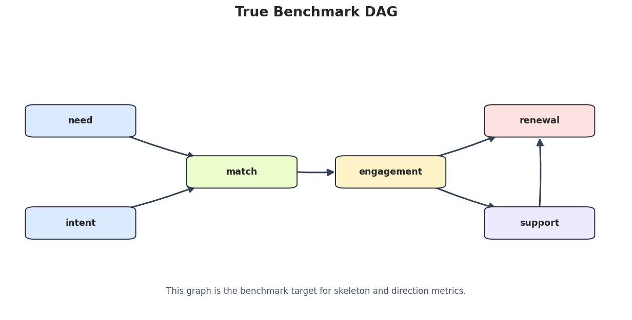
The benchmark graph has six variables and six directed edges. It is small enough to run many times, but rich enough to include a collider, a chain, and a downstream variable with two parents.

VARIABLES = ["need", "intent", "match", "engagement", "support", "renewal"]
VAR_INDEX = {name: i for i, name in enumerate(VARIABLES)}

TRUE_EDGES = [
    ("need", "match"),
    ("intent", "match"),
    ("match", "engagement"),
    ("engagement", "support"),
    ("engagement", "renewal"),
    ("support", "renewal"),
]

true_edge_table = pd.DataFrame(TRUE_EDGES, columns=["source", "target"])
true_edge_table["edge_type"] = "-->"
true_edge_table["run"] = "truth"
true_edge_table = true_edge_table[["run", "source", "edge_type", "target"]]
true_edge_table.to_csv(TABLE_DIR / f"{NOTEBOOK_PREFIX}_true_edges.csv", index=False)
display(true_edge_table)

	run	source	edge_type	target
0	truth	need	-->	match
1	truth	intent	-->	match
2	truth	match	-->	engagement
3	truth	engagement	-->	support
4	truth	engagement	-->	renewal
5	truth	support	-->	renewal

This truth table is used by all benchmark metrics. The same true graph is intentionally used across stress scenarios so we can see when violated assumptions create extra or missing observed relationships.

Simulate Data From The DAG

The simulator can generate several regimes from the same graph:

• linear Laplace noise for a baseline that favors DirectLiNGAM;
• linear Gaussian noise for Markov-equivalence-focused methods;
• nonlinear transformations for a simple functional misspecification check;
• hidden common causes that violate causal sufficiency.

The hidden-confounding regime should be read carefully: once a hidden common cause exists, the observed DAG is no longer a complete causal graph.

def draw_noise(rng, family, scale, n_samples):
    if family == "laplace":
        return rng.laplace(loc=0.0, scale=scale, size=n_samples)
    if family == "gaussian":
        return rng.normal(loc=0.0, scale=scale, size=n_samples)
    if family == "student_t":
        return rng.standard_t(df=4, size=n_samples) * scale / np.sqrt(2)
    raise ValueError(f"Unknown noise family: {family}")


def simulate_benchmark_data(
    n_samples=600,
    seed=RANDOM_SEED,
    noise_family="laplace",
    noise_scale=1.0,
    nonlinear=False,
    hidden_strength=0.0,
):
    """Simulate the six-variable benchmark graph."""
    rng = np.random.default_rng(seed)
    hidden = draw_noise(rng, noise_family, scale=1.0, n_samples=n_samples)

    need = draw_noise(rng, noise_family, noise_scale, n_samples) + hidden_strength * hidden
    intent = draw_noise(rng, noise_family, noise_scale, n_samples) + hidden_strength * hidden

    if nonlinear:
        match = 0.70 * np.tanh(need) + 0.60 * intent + draw_noise(rng, noise_family, noise_scale, n_samples)
        engagement = 0.75 * np.tanh(match) + draw_noise(rng, noise_family, noise_scale, n_samples)
    else:
        match = 0.70 * need + 0.60 * intent + draw_noise(rng, noise_family, noise_scale, n_samples)
        engagement = 0.75 * match + draw_noise(rng, noise_family, noise_scale, n_samples)

    support = -0.65 * engagement + draw_noise(rng, noise_family, noise_scale, n_samples)
    renewal = 0.65 * engagement - 0.45 * support + draw_noise(rng, noise_family, noise_scale, n_samples) + hidden_strength * hidden

    raw = pd.DataFrame(
        {
            "need": need,
            "intent": intent,
            "match": match,
            "engagement": engagement,
            "support": support,
            "renewal": renewal,
        }
    )
    scaled = pd.DataFrame(StandardScaler().fit_transform(raw), columns=VARIABLES)
    return scaled


baseline_df = simulate_benchmark_data(n_samples=600, seed=RANDOM_SEED, noise_family="laplace")
baseline_df.to_csv(DATASET_DIR / f"{NOTEBOOK_PREFIX}_baseline_linear_laplace.csv", index=False)
display(baseline_df.head())

	need	intent	match	engagement	support	renewal
0	-0.051522	0.054419	0.135313	0.193165	0.428653	-0.282088
1	0.463170	0.028769	0.415003	0.733303	-0.370460	-0.020052
2	1.054700	0.731401	0.225194	0.504820	-0.687442	0.540102
3	0.359936	0.349238	0.593094	1.194669	-0.439526	0.480990
4	1.687358	-2.190891	0.231224	0.628663	-1.310662	1.701560

The baseline data are standardized because PC, GES, and DirectLiNGAM all work more cleanly when variables are on comparable scales.

Baseline Data Audit

Before benchmarking algorithms, check the basic shape and correlation structure of the baseline data.

baseline_audit = pd.DataFrame(
    {
        "mean": baseline_df.mean(),
        "std": baseline_df.std(),
        "min": baseline_df.min(),
        "max": baseline_df.max(),
        "missing_rate": baseline_df.isna().mean(),
    }
).reset_index(names="variable")

baseline_corr = baseline_df.corr()
baseline_audit.to_csv(TABLE_DIR / f"{NOTEBOOK_PREFIX}_baseline_data_audit.csv", index=False)
baseline_corr.to_csv(TABLE_DIR / f"{NOTEBOOK_PREFIX}_baseline_correlation.csv")

display(baseline_audit.round(3))

fig, ax = plt.subplots(figsize=(8, 6))
sns.heatmap(baseline_corr, cmap="vlag", center=0, annot=True, fmt=".2f", square=True, ax=ax)
ax.set_title("Baseline Correlation Matrix")
plt.tight_layout()
fig.savefig(FIGURE_DIR / f"{NOTEBOOK_PREFIX}_baseline_correlation.png", dpi=160, bbox_inches="tight")
plt.show()

	variable	mean	std	min	max	missing_rate
0	need	0.0	1.001	-4.521	4.407	0.0
1	intent	-0.0	1.001	-4.537	4.370	0.0
2	match	-0.0	1.001	-3.492	3.720	0.0
3	engagement	0.0	1.001	-3.438	3.419	0.0
4	support	-0.0	1.001	-4.207	3.496	0.0
5	renewal	-0.0	1.001	-3.730	3.149	0.0

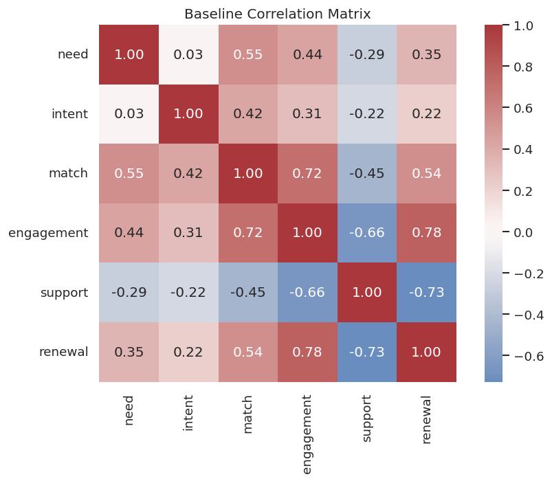
The correlation matrix shows strong relationships along the graph paths, but correlation alone cannot decide which adjacencies are direct or which way arrows point.

Draw The True DAG

The figure below is the benchmark target. The same box-and-arrow style is used across the tutorial series to keep graph outputs readable.

def trim_edge_to_box(start, end, box_w=0.15, box_h=0.085, gap=0.012):
    x0, y0 = start
    x1, y1 = end
    dx = x1 - x0
    dy = y1 - y0
    distance = (dx**2 + dy**2) ** 0.5
    if distance == 0:
        return start, end
    ux, uy = dx / distance, dy / distance
    candidates = []
    if abs(ux) > 1e-9:
        candidates.append((box_w / 2) / abs(ux))
    if abs(uy) > 1e-9:
        candidates.append((box_h / 2) / abs(uy))
    offset = min(candidates) + gap
    return (x0 + ux * offset, y0 + uy * offset), (x1 - ux * offset, y1 - uy * offset)


def draw_box_graph(edge_df, title, path, note=None):
    positions = {
        "need": (0.12, 0.68),
        "intent": (0.12, 0.32),
        "match": (0.38, 0.50),
        "engagement": (0.62, 0.50),
        "support": (0.86, 0.32),
        "renewal": (0.86, 0.68),
    }
    colors = {
        "need": "#dbeafe",
        "intent": "#dbeafe",
        "match": "#ecfccb",
        "engagement": "#fef3c7",
        "support": "#ede9fe",
        "renewal": "#fee2e2",
    }
    fig, ax = plt.subplots(figsize=(13, 6))
    ax.set_axis_off()
    ax.set_xlim(0, 1)
    ax.set_ylim(0, 1)

    for row in edge_df.itertuples(index=False):
        if row.source not in positions or row.target not in positions:
            continue
        start, end = trim_edge_to_box(positions[row.source], positions[row.target])
        edge_type = row.edge_type
        color = "#334155" if edge_type == "-->" else "#64748b"
        arrowstyle = "-|>" if edge_type == "-->" else "-"
        arrow = FancyArrowPatch(
            start,
            end,
            arrowstyle=arrowstyle,
            mutation_scale=17,
            linewidth=1.8,
            color=color,
            connectionstyle="arc3,rad=0.03",
            zorder=2,
        )
        ax.add_patch(arrow)

    for variable, (x, y) in positions.items():
        rect = FancyBboxPatch(
            (x - 0.075, y - 0.043),
            0.15,
            0.086,
            boxstyle="round,pad=0.014",
            facecolor=colors[variable],
            edgecolor="#1f2937",
            linewidth=1.15,
            zorder=4,
        )
        ax.add_patch(rect)
        ax.text(x, y, variable, ha="center", va="center", fontsize=10.5, fontweight="bold", zorder=5)

    if note:
        ax.text(0.5, 0.08, note, ha="center", va="center", fontsize=10, color="#475569")
    ax.set_title(title, pad=16, fontsize=16, fontweight="bold")
    fig.savefig(path, dpi=160, bbox_inches="tight")
    plt.show()


draw_box_graph(
    true_edge_table,
    "True Benchmark DAG",
    FIGURE_DIR / f"{NOTEBOOK_PREFIX}_true_benchmark_dag.png",
    note="This graph is the benchmark target for skeleton and direction metrics.",
)

This DAG is intentionally simple, but it contains enough structure to test adjacency recovery, collider handling, and downstream parent selection.

Graph Parsing And Metrics

The next helpers standardize graph outputs from PC, GES, FCI, and DirectLiNGAM. We score two layers:

• skeleton metrics: whether the correct variable pairs are adjacent;
• directed metrics: whether directed arrows match the true direction.

Partially directed or undirected edges count for skeleton recovery but not for directed recovery.

def parse_causallearn_edge(edge):
    text = str(edge).strip()
    edge_tokens = [" --> ", " <-- ", " <-> ", " o-> ", " <-o ", " o-o ", " --- "]
    for token in edge_tokens:
        if token in text:
            left, right = text.split(token)
            if token == " <-- ":
                return {"source": right.strip(), "edge_type": "-->", "target": left.strip()}
            if token == " <-o ":
                return {"source": right.strip(), "edge_type": "o->", "target": left.strip()}
            return {"source": left.strip(), "edge_type": token.strip(), "target": right.strip()}
    raise ValueError(f"Could not parse edge: {text}")


def graph_to_edge_table(graph, label):
    rows = [parse_causallearn_edge(edge) for edge in graph.get_graph_edges()]
    edge_table = pd.DataFrame(rows, columns=["source", "edge_type", "target"])
    edge_table.insert(0, "run", label)
    return edge_table


def lingam_to_edge_table(adjacency_matrix, label, threshold=0.12):
    rows = []
    for target in VARIABLES:
        for source in VARIABLES:
            if source == target:
                continue
            coefficient = float(adjacency_matrix[VAR_INDEX[target], VAR_INDEX[source]])
            if abs(coefficient) >= threshold:
                rows.append(
                    {
                        "run": label,
                        "source": source,
                        "edge_type": "-->",
                        "target": target,
                        "coefficient": coefficient,
                        "abs_coefficient": abs(coefficient),
                    }
                )
    return pd.DataFrame(rows, columns=["run", "source", "edge_type", "target", "coefficient", "abs_coefficient"])


def skeleton_pairs(edge_df):
    if edge_df.empty:
        return set()
    return {tuple(sorted((row.source, row.target))) for row in edge_df.itertuples(index=False)}


def directed_pairs(edge_df):
    if edge_df.empty:
        return set()
    return {(row.source, row.target) for row in edge_df.itertuples(index=False) if row.edge_type == "-->"}


TRUE_DIRECTED = set(TRUE_EDGES)
TRUE_SKELETON = {tuple(sorted(edge)) for edge in TRUE_EDGES}


def summarize_against_truth(edge_df, label, scenario="baseline"):
    learned_skeleton = skeleton_pairs(edge_df)
    learned_directed = directed_pairs(edge_df)
    skeleton_tp = learned_skeleton & TRUE_SKELETON
    skeleton_fp = learned_skeleton - TRUE_SKELETON
    skeleton_fn = TRUE_SKELETON - learned_skeleton
    directed_tp = learned_directed & TRUE_DIRECTED
    directed_fp = learned_directed - TRUE_DIRECTED
    directed_fn = TRUE_DIRECTED - learned_directed
    reversed_true_edges = {(target, source) for source, target in learned_directed} & TRUE_DIRECTED

    skeleton_precision = len(skeleton_tp) / len(learned_skeleton) if learned_skeleton else np.nan
    skeleton_recall = len(skeleton_tp) / len(TRUE_SKELETON)
    skeleton_f1 = 2 * skeleton_precision * skeleton_recall / (skeleton_precision + skeleton_recall) if skeleton_precision + skeleton_recall > 0 else np.nan
    directed_precision = len(directed_tp) / len(learned_directed) if learned_directed else np.nan
    directed_recall = len(directed_tp) / len(TRUE_DIRECTED)
    directed_f1 = 2 * directed_precision * directed_recall / (directed_precision + directed_recall) if directed_precision + directed_recall > 0 else np.nan

    return pd.DataFrame(
        [
            {
                "scenario": scenario,
                "method": label,
                "reported_edges": len(edge_df),
                "skeleton_precision": skeleton_precision,
                "skeleton_recall": skeleton_recall,
                "skeleton_f1": skeleton_f1,
                "directed_precision": directed_precision,
                "directed_recall": directed_recall,
                "directed_f1": directed_f1,
                "extra_adjacencies": len(skeleton_fp),
                "missed_adjacencies": len(skeleton_fn),
                "reversed_true_edges": len(reversed_true_edges),
                "extra_adjacency_list": " | ".join(f"{a}--{b}" for a, b in sorted(skeleton_fp)),
                "missed_adjacency_list": " | ".join(f"{a}--{b}" for a, b in sorted(skeleton_fn)),
            }
        ]
    )

The metric functions make the benchmark transparent. A partially directed PC or GES graph can still score well on skeleton recovery while receiving lower directed recall.

Algorithm Runners

This cell wraps PC, GES, FCI, and DirectLiNGAM so later benchmark grids can call them consistently. We keep the defaults conservative and expose the main tuning knobs.

def run_pc(data_df, alpha=0.01, label="PC_FisherZ"):
    start = time.perf_counter()
    result = pc(
        data_df.to_numpy(),
        alpha=alpha,
        indep_test="fisherz",
        stable=True,
        show_progress=False,
        node_names=VARIABLES,
    )
    elapsed = time.perf_counter() - start
    return graph_to_edge_table(result.G, label), elapsed


def run_ges(data_df, lambda_value=1.0, label="GES_BIC"):
    start = time.perf_counter()
    record = ges(
        data_df.to_numpy(),
        score_func="local_score_BIC_from_cov",
        node_names=VARIABLES,
        parameters={"lambda_value": lambda_value},
    )
    elapsed = time.perf_counter() - start
    return graph_to_edge_table(record["G"], label), elapsed


def run_direct_lingam(data_df, threshold=0.12, label="DirectLiNGAM"):
    start = time.perf_counter()
    model = DirectLiNGAM(random_state=RANDOM_SEED)
    model.fit(data_df.to_numpy())
    elapsed = time.perf_counter() - start
    edge_table = lingam_to_edge_table(model.adjacency_matrix_, label=label, threshold=threshold)
    return edge_table, elapsed, model


def run_fci(data_df, alpha=0.01, label="FCI_FisherZ"):
    start = time.perf_counter()
    graph, _ = fci(
        data_df.to_numpy(),
        independence_test_method="fisherz",
        alpha=alpha,
        show_progress=False,
        node_names=VARIABLES,
    )
    elapsed = time.perf_counter() - start
    return graph_to_edge_table(graph, label), elapsed


def run_benchmark_methods(data_df, scenario="baseline", pc_alpha=0.01, ges_lambda=1.0, lingam_threshold=0.12):
    rows = []
    edges = []

    pc_edges, pc_elapsed = run_pc(data_df, alpha=pc_alpha, label="PC_FisherZ")
    rows.append(summarize_against_truth(pc_edges, "PC_FisherZ", scenario).assign(elapsed_seconds=pc_elapsed))
    edges.append(pc_edges.assign(scenario=scenario, elapsed_seconds=pc_elapsed))

    ges_edges, ges_elapsed = run_ges(data_df, lambda_value=ges_lambda, label="GES_BIC")
    rows.append(summarize_against_truth(ges_edges, "GES_BIC", scenario).assign(elapsed_seconds=ges_elapsed))
    edges.append(ges_edges.assign(scenario=scenario, elapsed_seconds=ges_elapsed))

    lingam_edges, lingam_elapsed, _ = run_direct_lingam(data_df, threshold=lingam_threshold, label="DirectLiNGAM")
    rows.append(summarize_against_truth(lingam_edges, "DirectLiNGAM", scenario).assign(elapsed_seconds=lingam_elapsed))
    edges.append(lingam_edges.assign(scenario=scenario, elapsed_seconds=lingam_elapsed))

    return pd.concat(rows, ignore_index=True), pd.concat(edges, ignore_index=True)

These wrappers are intentionally small. They avoid hidden defaults in the benchmark loops and make each algorithm’s tuning parameters visible.

Baseline Algorithm Comparison

Now we run PC, GES, and DirectLiNGAM on the same baseline data. This is the cleanest comparison because the data are linear, acyclic, causally sufficient, and non-Gaussian.

baseline_metrics, baseline_edges = run_benchmark_methods(baseline_df, scenario="linear_laplace_baseline")
baseline_metrics.to_csv(TABLE_DIR / f"{NOTEBOOK_PREFIX}_baseline_method_metrics.csv", index=False)
baseline_edges.to_csv(TABLE_DIR / f"{NOTEBOOK_PREFIX}_baseline_method_edges.csv", index=False)

display(baseline_metrics.round(4))
display(baseline_edges)

	scenario	method	reported_edges	skeleton_precision	skeleton_recall	skeleton_f1	directed_precision	directed_recall	directed_f1	extra_adjacencies	missed_adjacencies	reversed_true_edges	extra_adjacency_list	missed_adjacency_list	elapsed_seconds
0	linear_laplace_baseline	PC_FisherZ	6	1.0	1.0	1.0	1.0	0.8333	0.9091	0	0	0			0.0070
1	linear_laplace_baseline	GES_BIC	6	1.0	1.0	1.0	1.0	0.8333	0.9091	0	0	0			0.0116
2	linear_laplace_baseline	DirectLiNGAM	6	1.0	1.0	1.0	1.0	1.0000	1.0000	0	0	0			0.0247

	run	source	edge_type	target	scenario	elapsed_seconds	coefficient	abs_coefficient
0	PC_FisherZ	need	-->	match	linear_laplace_baseline	0.006988	NaN	NaN
1	PC_FisherZ	intent	-->	match	linear_laplace_baseline	0.006988	NaN	NaN
2	PC_FisherZ	match	-->	engagement	linear_laplace_baseline	0.006988	NaN	NaN
3	PC_FisherZ	engagement	-->	support	linear_laplace_baseline	0.006988	NaN	NaN
4	PC_FisherZ	engagement	-->	renewal	linear_laplace_baseline	0.006988	NaN	NaN
5	PC_FisherZ	support	---	renewal	linear_laplace_baseline	0.006988	NaN	NaN
6	GES_BIC	need	-->	match	linear_laplace_baseline	0.011578	NaN	NaN
7	GES_BIC	intent	-->	match	linear_laplace_baseline	0.011578	NaN	NaN
8	GES_BIC	match	-->	engagement	linear_laplace_baseline	0.011578	NaN	NaN
9	GES_BIC	engagement	-->	support	linear_laplace_baseline	0.011578	NaN	NaN
10	GES_BIC	engagement	-->	renewal	linear_laplace_baseline	0.011578	NaN	NaN
11	GES_BIC	support	---	renewal	linear_laplace_baseline	0.011578	NaN	NaN
12	DirectLiNGAM	need	-->	match	linear_laplace_baseline	0.024743	0.534778	0.534778
13	DirectLiNGAM	intent	-->	match	linear_laplace_baseline	0.024743	0.409543	0.409543
14	DirectLiNGAM	match	-->	engagement	linear_laplace_baseline	0.024743	0.709682	0.709682
15	DirectLiNGAM	engagement	-->	support	linear_laplace_baseline	0.024743	-0.657750	0.657750
16	DirectLiNGAM	engagement	-->	renewal	linear_laplace_baseline	0.024743	0.537382	0.537382
17	DirectLiNGAM	support	-->	renewal	linear_laplace_baseline	0.024743	-0.371057	0.371057

The baseline is deliberately friendly to all three methods. PC and GES usually recover the correct skeleton and many directions; DirectLiNGAM can recover all directions because the data match its linear non-Gaussian assumptions.

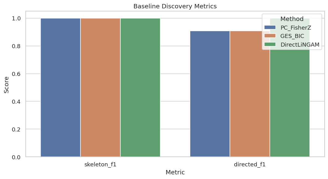
Plot Baseline Metrics

A compact metric plot lets us see the skeleton-versus-direction distinction immediately.

baseline_plot = baseline_metrics.melt(
    id_vars="method",
    value_vars=["skeleton_f1", "directed_f1"],
    var_name="metric",
    value_name="score",
)

fig, ax = plt.subplots(figsize=(9, 5))
sns.barplot(data=baseline_plot, x="metric", y="score", hue="method", ax=ax)
ax.set_title("Baseline Discovery Metrics")
ax.set_xlabel("Metric")
ax.set_ylabel("Score")
ax.set_ylim(0, 1.05)
ax.legend(title="Method")
plt.tight_layout()
fig.savefig(FIGURE_DIR / f"{NOTEBOOK_PREFIX}_baseline_method_metrics.png", dpi=160, bbox_inches="tight")
plt.show()

The plot shows why benchmark reports should not collapse everything into one number. Recovering adjacencies and orienting arrows are related but different tasks.

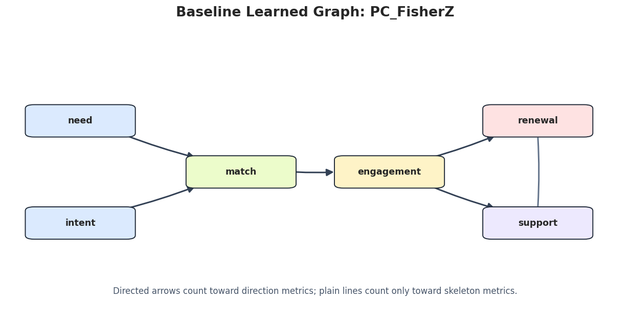
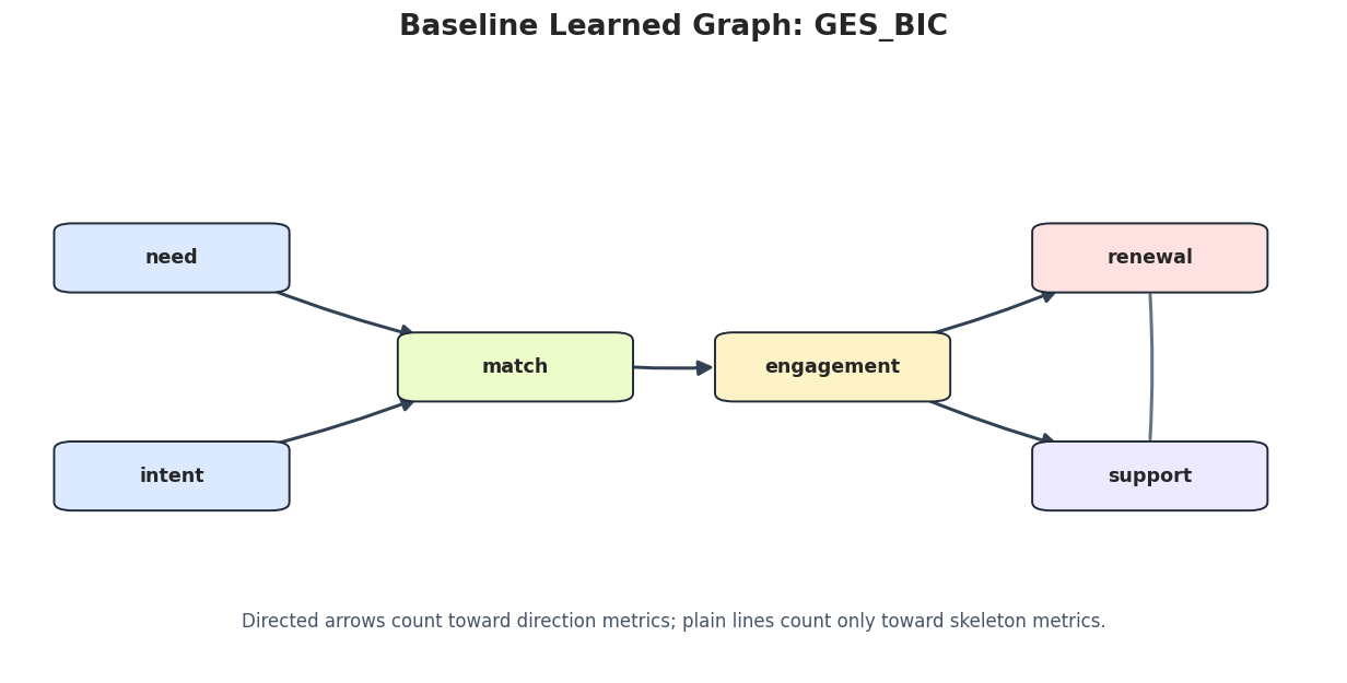
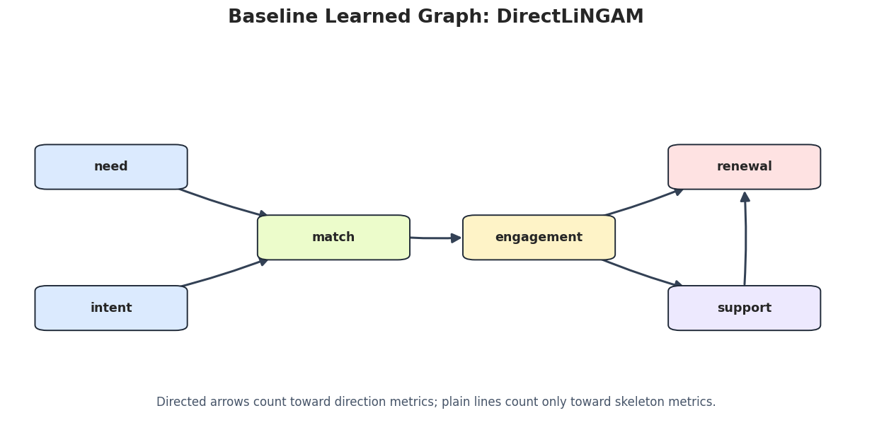
Draw Baseline Learned Graphs

The next cell saves one graph image per method. Undirected or partially oriented edges are drawn as plain lines so they are not mistaken for confirmed arrow directions.

for method_name in baseline_edges["run"].unique():
    method_edges = baseline_edges[baseline_edges["run"] == method_name].copy()
    draw_box_graph(
        method_edges,
        f"Baseline Learned Graph: {method_name}",
        FIGURE_DIR / f"{NOTEBOOK_PREFIX}_baseline_{method_name.lower()}_graph.png",
        note="Directed arrows count toward direction metrics; plain lines count only toward skeleton metrics.",
    )

These plots are useful for qualitative review. The metric table tells us what changed; the graph drawings make the change easier to inspect.

Sample-Size And Seed Stability

A stable discovery method should not depend on one lucky sample. This grid varies sample size and random seed, then reruns all three benchmark methods.

stability_metric_rows = []
stability_edge_rows = []
for n_samples in [150, 300, 600, 1_000]:
    for seed in range(3):
        sample_df = simulate_benchmark_data(n_samples=n_samples, seed=seed, noise_family="laplace")
        metrics, edges = run_benchmark_methods(sample_df, scenario=f"n_{n_samples}_seed_{seed}")
        metrics["n_samples"] = n_samples
        metrics["seed"] = seed
        edges["n_samples"] = n_samples
        edges["seed"] = seed
        stability_metric_rows.append(metrics)
        stability_edge_rows.append(edges)

sample_seed_metrics = pd.concat(stability_metric_rows, ignore_index=True)
sample_seed_edges = pd.concat(stability_edge_rows, ignore_index=True)
sample_seed_summary = sample_seed_metrics.groupby(["method", "n_samples"], as_index=False).agg(
    runs=("seed", "count"),
    mean_skeleton_f1=("skeleton_f1", "mean"),
    min_skeleton_f1=("skeleton_f1", "min"),
    mean_directed_f1=("directed_f1", "mean"),
    min_directed_f1=("directed_f1", "min"),
    mean_elapsed_seconds=("elapsed_seconds", "mean"),
)

sample_seed_metrics.to_csv(TABLE_DIR / f"{NOTEBOOK_PREFIX}_sample_seed_metrics.csv", index=False)
sample_seed_edges.to_csv(TABLE_DIR / f"{NOTEBOOK_PREFIX}_sample_seed_edges.csv", index=False)
sample_seed_summary.to_csv(TABLE_DIR / f"{NOTEBOOK_PREFIX}_sample_seed_summary.csv", index=False)

display(sample_seed_summary.round(4))

	method	n_samples	runs	mean_skeleton_f1	min_skeleton_f1	mean_directed_f1	min_directed_f1	mean_elapsed_seconds
0	DirectLiNGAM	150	3	1.0000	1.0000	1.0000	1.0000	0.0190
1	DirectLiNGAM	300	3	1.0000	1.0000	1.0000	1.0000	0.0200
2	DirectLiNGAM	600	3	1.0000	1.0000	1.0000	1.0000	0.0223
3	DirectLiNGAM	1000	3	1.0000	1.0000	1.0000	1.0000	0.0240
4	GES_BIC	150	3	1.0000	1.0000	0.9091	0.9091	0.0118
5	GES_BIC	300	3	1.0000	1.0000	0.9091	0.9091	0.0119
6	GES_BIC	600	3	1.0000	1.0000	0.9091	0.9091	0.0125
7	GES_BIC	1000	3	0.9744	0.9231	0.9138	0.9091	0.0138
8	PC_FisherZ	150	3	0.9697	0.9091	0.8485	0.7273	0.0098
9	PC_FisherZ	300	3	1.0000	1.0000	0.9091	0.9091	0.0065
10	PC_FisherZ	600	3	1.0000	1.0000	0.9091	0.9091	0.0072
11	PC_FisherZ	1000	3	1.0000	1.0000	0.9091	0.9091	0.0070

The summary shows how recovery improves as the sample grows. Small samples can preserve the rough skeleton while making directions less reliable.

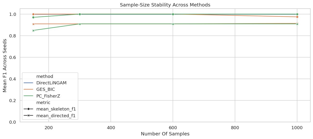
Plot Sample-Size Stability

The line plot uses the mean F1 scores across seeds for each sample size.

sample_plot = sample_seed_summary.melt(
    id_vars=["method", "n_samples"],
    value_vars=["mean_skeleton_f1", "mean_directed_f1"],
    var_name="metric",
    value_name="score",
)

fig, ax = plt.subplots(figsize=(11, 5))
sns.lineplot(data=sample_plot, x="n_samples", y="score", hue="method", style="metric", markers=True, dashes=False, ax=ax)
ax.set_title("Sample-Size Stability Across Methods")
ax.set_xlabel("Number Of Samples")
ax.set_ylabel("Mean F1 Across Seeds")
ax.set_ylim(0, 1.05)
plt.tight_layout()
fig.savefig(FIGURE_DIR / f"{NOTEBOOK_PREFIX}_sample_size_stability.png", dpi=160, bbox_inches="tight")
plt.show()

The plot makes the practical sample-size story visible. If the directed score is unstable at small n, a report should avoid strong directional claims from that region.

Noise Sensitivity

Next we hold sample size fixed and vary the measurement noise scale. Higher noise weakens the signal-to-noise ratio and can make direct adjacencies harder to recover.

noise_metric_rows = []
for noise_scale in [0.60, 1.00, 1.40, 1.80]:
    sample_df = simulate_benchmark_data(n_samples=600, seed=RANDOM_SEED, noise_family="laplace", noise_scale=noise_scale)
    metrics, _ = run_benchmark_methods(sample_df, scenario=f"noise_{noise_scale:.2f}")
    metrics["noise_scale"] = noise_scale
    noise_metric_rows.append(metrics)

noise_sensitivity = pd.concat(noise_metric_rows, ignore_index=True)
noise_sensitivity.to_csv(TABLE_DIR / f"{NOTEBOOK_PREFIX}_noise_sensitivity.csv", index=False)
display(noise_sensitivity[["method", "noise_scale", "skeleton_f1", "directed_f1", "extra_adjacencies", "missed_adjacencies", "reversed_true_edges"]].round(4))

	method	noise_scale	skeleton_f1	directed_f1	extra_adjacencies	missed_adjacencies	reversed_true_edges
0	PC_FisherZ	0.6	1.0	0.9091	0	0	0
1	GES_BIC	0.6	1.0	0.9091	0	0	0
2	DirectLiNGAM	0.6	1.0	1.0000	0	0	0
3	PC_FisherZ	1.0	1.0	0.9091	0	0	0
4	GES_BIC	1.0	1.0	0.9091	0	0	0
5	DirectLiNGAM	1.0	1.0	1.0000	0	0	0
6	PC_FisherZ	1.4	1.0	0.9091	0	0	0
7	GES_BIC	1.4	1.0	0.9091	0	0	0
8	DirectLiNGAM	1.4	1.0	1.0000	0	0	0
9	PC_FisherZ	1.8	1.0	0.9091	0	0	0
10	GES_BIC	1.8	1.0	0.9091	0	0	0
11	DirectLiNGAM	1.8	1.0	1.0000	0	0	0

Noise sensitivity is a useful robustness check because real datasets rarely have the clean signal strength used in synthetic demos.

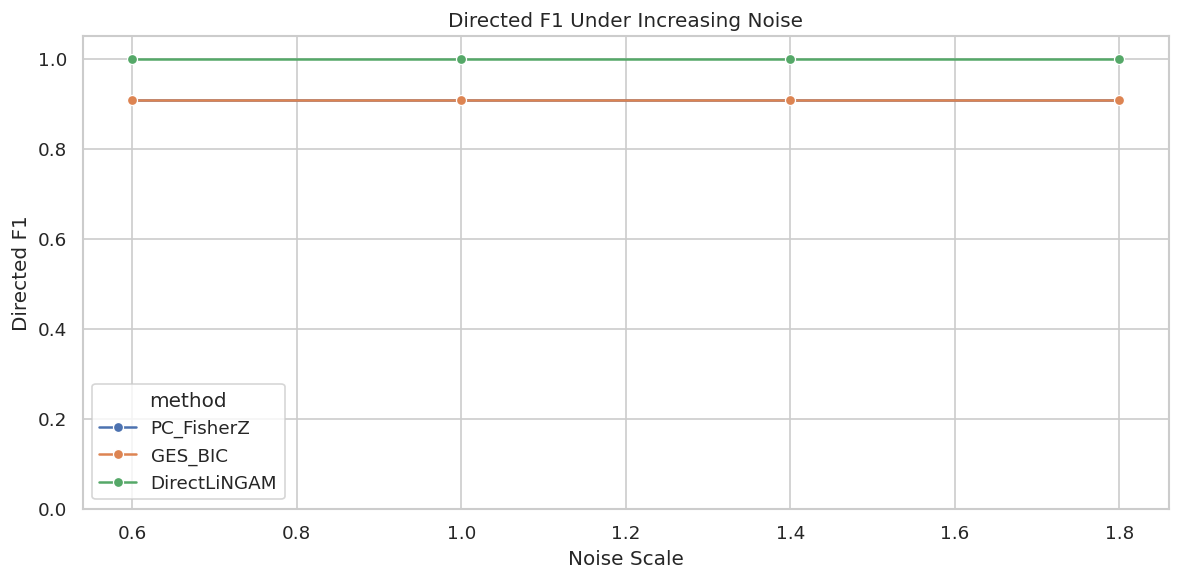
Plot Noise Sensitivity

The next figure tracks directed F1 as noise increases. Skeleton scores are saved in the table above; the directed score is usually the more fragile layer.

fig, ax = plt.subplots(figsize=(10, 5))
sns.lineplot(data=noise_sensitivity, x="noise_scale", y="directed_f1", hue="method", marker="o", ax=ax)
ax.set_title("Directed F1 Under Increasing Noise")
ax.set_xlabel("Noise Scale")
ax.set_ylabel("Directed F1")
ax.set_ylim(0, 1.05)
plt.tight_layout()
fig.savefig(FIGURE_DIR / f"{NOTEBOOK_PREFIX}_noise_sensitivity.png", dpi=160, bbox_inches="tight")
plt.show()

If a method’s directed score drops sharply as noise increases, its arrow claims should be reported with caution in low-signal applications.

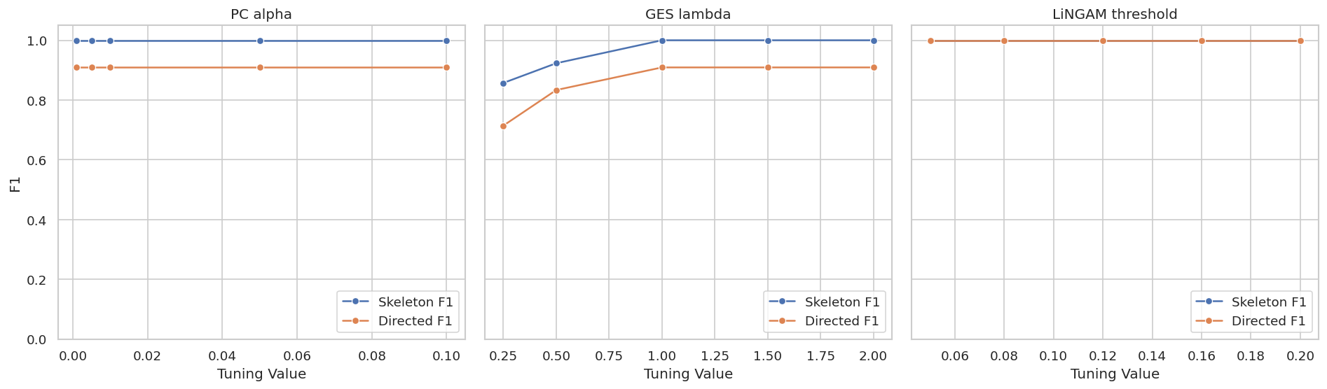
Tuning Sensitivity: PC Alpha

PC depends on a conditional-independence significance level. Larger alpha values tend to remove fewer edges, while smaller values tend to remove more edges. The right value is data-dependent, so it should be scanned rather than hidden.

pc_alpha_rows = []
for alpha in [0.001, 0.005, 0.01, 0.05, 0.10]:
    edges, elapsed = run_pc(baseline_df, alpha=alpha, label="PC_FisherZ")
    metrics = summarize_against_truth(edges, "PC_FisherZ", scenario=f"pc_alpha_{alpha}")
    metrics["alpha"] = alpha
    metrics["elapsed_seconds"] = elapsed
    pc_alpha_rows.append(metrics)

pc_alpha_sensitivity = pd.concat(pc_alpha_rows, ignore_index=True)
pc_alpha_sensitivity.to_csv(TABLE_DIR / f"{NOTEBOOK_PREFIX}_pc_alpha_sensitivity.csv", index=False)
display(pc_alpha_sensitivity[["alpha", "reported_edges", "skeleton_f1", "directed_f1", "extra_adjacencies", "missed_adjacencies"]].round(4))

	alpha	reported_edges	skeleton_f1	directed_f1	extra_adjacencies	missed_adjacencies
0	0.001	6	1.0	0.9091	0	0
1	0.005	6	1.0	0.9091	0	0
2	0.010	6	1.0	0.9091	0	0
3	0.050	6	1.0	0.9091	0	0
4	0.100	6	1.0	0.9091	0	0

The PC alpha scan shows whether the learned graph is stable across reasonable independence-test thresholds.

Tuning Sensitivity: GES Penalty

GES uses a score penalty. Larger penalties favor simpler graphs. Smaller penalties can admit extra edges. We scan the penalty multiplier used by the local BIC score.

ges_lambda_rows = []
for lambda_value in [0.25, 0.50, 1.00, 1.50, 2.00]:
    edges, elapsed = run_ges(baseline_df, lambda_value=lambda_value, label="GES_BIC")
    metrics = summarize_against_truth(edges, "GES_BIC", scenario=f"ges_lambda_{lambda_value}")
    metrics["lambda_value"] = lambda_value
    metrics["elapsed_seconds"] = elapsed
    ges_lambda_rows.append(metrics)

ges_lambda_sensitivity = pd.concat(ges_lambda_rows, ignore_index=True)
ges_lambda_sensitivity.to_csv(TABLE_DIR / f"{NOTEBOOK_PREFIX}_ges_lambda_sensitivity.csv", index=False)
display(ges_lambda_sensitivity[["lambda_value", "reported_edges", "skeleton_f1", "directed_f1", "extra_adjacencies", "missed_adjacencies"]].round(4))

	lambda_value	reported_edges	skeleton_f1	directed_f1	extra_adjacencies	missed_adjacencies
0	0.25	8	0.8571	0.7143	2	0
1	0.50	7	0.9231	0.8333	1	0
2	1.00	6	1.0000	0.9091	0	0
3	1.50	6	1.0000	0.9091	0	0
4	2.00	6	1.0000	0.9091	0	0

The GES penalty scan makes the sparsity tradeoff explicit. A benchmark should say which penalty produced the reported graph.

Tuning Sensitivity: DirectLiNGAM Coefficient Threshold

DirectLiNGAM returns a weighted adjacency matrix. To report a graph, we need a coefficient threshold. This cell fits DirectLiNGAM once and scans several thresholds.

_, _, baseline_lingam_model = run_direct_lingam(baseline_df, threshold=0.12, label="DirectLiNGAM")
lingam_threshold_rows = []
lingam_threshold_edges = []
for threshold in [0.05, 0.08, 0.12, 0.16, 0.20]:
    edges = lingam_to_edge_table(baseline_lingam_model.adjacency_matrix_, label="DirectLiNGAM", threshold=threshold)
    metrics = summarize_against_truth(edges, "DirectLiNGAM", scenario=f"lingam_threshold_{threshold}")
    metrics["threshold"] = threshold
    lingam_threshold_rows.append(metrics)
    lingam_threshold_edges.append(edges.assign(threshold=threshold))

lingam_threshold_sensitivity = pd.concat(lingam_threshold_rows, ignore_index=True)
lingam_threshold_edge_table = pd.concat(lingam_threshold_edges, ignore_index=True)
lingam_threshold_sensitivity.to_csv(TABLE_DIR / f"{NOTEBOOK_PREFIX}_lingam_threshold_sensitivity.csv", index=False)
lingam_threshold_edge_table.to_csv(TABLE_DIR / f"{NOTEBOOK_PREFIX}_lingam_threshold_edges.csv", index=False)
display(lingam_threshold_sensitivity[["threshold", "reported_edges", "skeleton_f1", "directed_f1", "extra_adjacencies", "missed_adjacencies"]].round(4))

	threshold	reported_edges	skeleton_f1	directed_f1	extra_adjacencies	missed_adjacencies
0	0.05	6	1.0	1.0	0	0
1	0.08	6	1.0	1.0	0	0
2	0.12	6	1.0	1.0	0	0
3	0.16	6	1.0	1.0	0	0
4	0.20	6	1.0	1.0	0	0

The threshold scan is a reminder that weighted-output algorithms still require a reporting rule. A low threshold can over-report weak edges; a high threshold can drop true but weaker effects.

Plot Tuning Sensitivity

This plot puts the main tuning scans on one page. Each panel uses the method-specific tuning parameter, so read the x-axis labels separately.

tuning_plot_frames = [
    pc_alpha_sensitivity.assign(tuning_family="PC alpha", tuning_value=pc_alpha_sensitivity["alpha"]),
    ges_lambda_sensitivity.assign(tuning_family="GES lambda", tuning_value=ges_lambda_sensitivity["lambda_value"]),
    lingam_threshold_sensitivity.assign(tuning_family="LiNGAM threshold", tuning_value=lingam_threshold_sensitivity["threshold"]),
]
tuning_plot = pd.concat(tuning_plot_frames, ignore_index=True)

fig, axes = plt.subplots(1, 3, figsize=(16, 4.8), sharey=True)
for ax, family in zip(axes, ["PC alpha", "GES lambda", "LiNGAM threshold"]):
    subset = tuning_plot[tuning_plot["tuning_family"] == family]
    sns.lineplot(data=subset, x="tuning_value", y="skeleton_f1", marker="o", label="Skeleton F1", ax=ax)
    sns.lineplot(data=subset, x="tuning_value", y="directed_f1", marker="o", label="Directed F1", ax=ax)
    ax.set_title(family)
    ax.set_xlabel("Tuning Value")
    ax.set_ylabel("F1")
    ax.set_ylim(0, 1.05)
    ax.legend(loc="lower right")
plt.tight_layout()
fig.savefig(FIGURE_DIR / f"{NOTEBOOK_PREFIX}_tuning_sensitivity.png", dpi=160, bbox_inches="tight")
plt.show()

Stable regions are more reassuring than isolated peaks. In an applied report, a graph chosen from a narrow peak should be described as sensitive to tuning.

Assumption Stress Scenarios

The baseline was friendly. Now we deliberately perturb the assumptions:

• linear_laplace: baseline linear non-Gaussian data;
• linear_gaussian: directions are harder for LiNGAM because non-Gaussianity is removed;
• nonlinear_laplace: linear algorithms are misspecified;
• hidden_confounding: causal sufficiency is violated by an unobserved common cause.

The hidden-confounding scores are not a fair observed-DAG target; they are included to show how observed-DAG methods can become unstable when a key assumption fails.

stress_configs = [
    {"scenario": "linear_laplace", "noise_family": "laplace", "nonlinear": False, "hidden_strength": 0.0},
    {"scenario": "linear_gaussian", "noise_family": "gaussian", "nonlinear": False, "hidden_strength": 0.0},
    {"scenario": "nonlinear_laplace", "noise_family": "laplace", "nonlinear": True, "hidden_strength": 0.0},
    {"scenario": "hidden_confounding", "noise_family": "laplace", "nonlinear": False, "hidden_strength": 1.0},
]

stress_metric_rows = []
stress_edge_rows = []
for config in stress_configs:
    scenario_df = simulate_benchmark_data(
        n_samples=700,
        seed=3,
        noise_family=config["noise_family"],
        nonlinear=config["nonlinear"],
        hidden_strength=config["hidden_strength"],
    )
    scenario_df.to_csv(DATASET_DIR / f"{NOTEBOOK_PREFIX}_{config['scenario']}.csv", index=False)
    metrics, edges = run_benchmark_methods(scenario_df, scenario=config["scenario"])
    metrics["noise_family"] = config["noise_family"]
    metrics["nonlinear"] = config["nonlinear"]
    metrics["hidden_strength"] = config["hidden_strength"]
    stress_metric_rows.append(metrics)
    stress_edge_rows.append(edges)

stress_metrics = pd.concat(stress_metric_rows, ignore_index=True)
stress_edges = pd.concat(stress_edge_rows, ignore_index=True)
stress_metrics.to_csv(TABLE_DIR / f"{NOTEBOOK_PREFIX}_assumption_stress_metrics.csv", index=False)
stress_edges.to_csv(TABLE_DIR / f"{NOTEBOOK_PREFIX}_assumption_stress_edges.csv", index=False)

display(stress_metrics[["scenario", "method", "skeleton_f1", "directed_f1", "extra_adjacencies", "missed_adjacencies", "reversed_true_edges"]].round(4))

	scenario	method	skeleton_f1	directed_f1	extra_adjacencies	missed_adjacencies	reversed_true_edges
0	linear_laplace	PC_FisherZ	1.0000	0.9091	0	0	0
1	linear_laplace	GES_BIC	0.9231	0.9231	1	0	0
2	linear_laplace	DirectLiNGAM	1.0000	1.0000	0	0	0
3	linear_gaussian	PC_FisherZ	1.0000	0.9091	0	0	0
4	linear_gaussian	GES_BIC	1.0000	0.9091	0	0	0
5	linear_gaussian	DirectLiNGAM	0.8571	0.4286	2	0	3
6	nonlinear_laplace	PC_FisherZ	1.0000	0.9091	0	0	0
7	nonlinear_laplace	GES_BIC	1.0000	0.9091	0	0	0
8	nonlinear_laplace	DirectLiNGAM	0.9231	0.7692	1	0	1
9	hidden_confounding	PC_FisherZ	0.8000	0.3636	3	0	1
10	hidden_confounding	GES_BIC	0.7500	0.3333	4	0	1
11	hidden_confounding	DirectLiNGAM	0.7500	0.5000	4	0	2

The stress table shows which failures are algorithm-specific and which are assumption-level. Gaussian noise mainly weakens DirectLiNGAM direction recovery; hidden confounding can create extra adjacencies or misleading directions for observed-DAG methods.

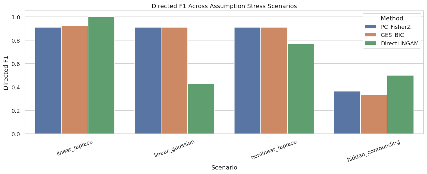
Plot Assumption Stress Results

The next figure compares directed F1 across the stress scenarios. Skeleton details are saved in the table above.

fig, ax = plt.subplots(figsize=(12, 5))
sns.barplot(data=stress_metrics, x="scenario", y="directed_f1", hue="method", ax=ax)
ax.set_title("Directed F1 Across Assumption Stress Scenarios")
ax.set_xlabel("Scenario")
ax.set_ylabel("Directed F1")
ax.set_ylim(0, 1.05)
ax.tick_params(axis="x", rotation=20)
ax.legend(title="Method")
plt.tight_layout()
fig.savefig(FIGURE_DIR / f"{NOTEBOOK_PREFIX}_assumption_stress_directed_f1.png", dpi=160, bbox_inches="tight")
plt.show()

The plot turns the warning into something visible. A method that performs beautifully under one data-generating regime can become much less reliable under another.

Targeted Hidden-Confounding Check With FCI

FCI is designed for settings where hidden common causes may exist. This cell runs FCI only on the hidden-confounding scenario. The goal is not to score FCI against the same observed DAG, because the target graph type is different. The goal is to inspect whether the output marks possible hidden structure.

hidden_df = pd.read_csv(DATASET_DIR / f"{NOTEBOOK_PREFIX}_hidden_confounding.csv")
fci_edges, fci_elapsed = run_fci(hidden_df, alpha=0.01, label="FCI_FisherZ_hidden")
fci_edges["elapsed_seconds"] = fci_elapsed
fci_edges.to_csv(TABLE_DIR / f"{NOTEBOOK_PREFIX}_hidden_fci_edges.csv", index=False)
display(fci_edges)
print(f"FCI elapsed seconds: {fci_elapsed:.4f}")

renewal --> support

	run	source	edge_type	target	elapsed_seconds
0	FCI_FisherZ_hidden	need	o-o	intent	0.016929
1	FCI_FisherZ_hidden	need	o-o	match	0.016929
2	FCI_FisherZ_hidden	need	o->	renewal	0.016929
3	FCI_FisherZ_hidden	intent	o-o	match	0.016929
4	FCI_FisherZ_hidden	intent	o->	renewal	0.016929
5	FCI_FisherZ_hidden	match	o-o	engagement	0.016929
6	FCI_FisherZ_hidden	engagement	-->	support	0.016929
7	FCI_FisherZ_hidden	engagement	-->	renewal	0.016929
8	FCI_FisherZ_hidden	renewal	-->	support	0.016929

FCI elapsed seconds: 0.0169

FCI uses endpoint marks that should be read differently from a DAG. Bidirected or partially marked edges are signs that hidden structure may be involved, not ordinary directed arrows from the observed DAG benchmark.

Edge Stability Signatures

Stability can also be summarized by graph signatures. The next cell counts how many unique graphs each method produced across the sample-size and seed grid.

def edge_signature(edge_df):
    if edge_df.empty:
        return "empty"
    return " | ".join(sorted(f"{row.source} {row.edge_type} {row.target}" for row in edge_df.itertuples(index=False)))

signature_rows = []
for (method, n_samples, seed), group in sample_seed_edges.groupby(["run", "n_samples", "seed"]):
    signature_rows.append(
        {
            "method": method,
            "n_samples": n_samples,
            "seed": seed,
            "edge_signature": edge_signature(group),
            "reported_edges": len(group),
        }
    )

signature_table = pd.DataFrame(signature_rows)
signature_summary = signature_table.groupby(["method", "n_samples"], as_index=False).agg(
    unique_graphs=("edge_signature", "nunique"),
    min_reported_edges=("reported_edges", "min"),
    max_reported_edges=("reported_edges", "max"),
)
signature_table.to_csv(TABLE_DIR / f"{NOTEBOOK_PREFIX}_edge_signatures.csv", index=False)
signature_summary.to_csv(TABLE_DIR / f"{NOTEBOOK_PREFIX}_edge_signature_summary.csv", index=False)
display(signature_summary)

	method	n_samples	unique_graphs	min_reported_edges	max_reported_edges
0	DirectLiNGAM	150	1	6	6
1	DirectLiNGAM	300	1	6	6
2	DirectLiNGAM	600	1	6	6
3	DirectLiNGAM	1000	1	6	6
4	GES_BIC	150	1	6	6
5	GES_BIC	300	1	6	6
6	GES_BIC	600	1	6	6
7	GES_BIC	1000	2	6	7
8	PC_FisherZ	150	2	5	6
9	PC_FisherZ	300	1	6	6
10	PC_FisherZ	600	1	6	6
11	PC_FisherZ	1000	1	6	6

Unique graph counts help distinguish stable metrics from stable graphs. Two graphs can have the same F1 score but disagree about which specific edge changed.

Runtime Summary

Runtime is part of method selection. A method that is statistically attractive but too slow for repeated sensitivity checks may be hard to use responsibly on a larger graph.

runtime_summary = pd.concat(
    [
        baseline_metrics.assign(source_table="baseline"),
        sample_seed_metrics.assign(source_table="sample_seed"),
        noise_sensitivity.assign(source_table="noise"),
        stress_metrics.assign(source_table="stress"),
    ],
    ignore_index=True,
).groupby("method", as_index=False).agg(
    runs=("elapsed_seconds", "count"),
    median_elapsed_seconds=("elapsed_seconds", "median"),
    max_elapsed_seconds=("elapsed_seconds", "max"),
)
runtime_summary.to_csv(TABLE_DIR / f"{NOTEBOOK_PREFIX}_runtime_summary.csv", index=False)
display(runtime_summary.round(4))

	method	runs	median_elapsed_seconds	max_elapsed_seconds
0	DirectLiNGAM	21	0.0221	0.0254
1	GES_BIC	21	0.0120	0.0207
2	PC_FisherZ	21	0.0070	0.0114

The runtime table is small here because the graph has only six variables. On wider graphs, runtime and stability checks become a much bigger part of practical method choice.

Benchmark Reporting Checklist

A benchmark should make its assumptions and fragility visible. This checklist is a reusable template for reporting causal discovery comparisons.

reporting_checklist = pd.DataFrame(
    [
        {
            "item": "Graph target",
            "what_to_report": "Whether metrics target a DAG, CPDAG, PAG, skeleton, or weighted adjacency matrix.",
            "why_it_matters": "Different algorithms return different graph objects and should not be collapsed casually.",
        },
        {
            "item": "Data-generating assumptions",
            "what_to_report": "Linearity, noise family, causal sufficiency, stationarity, and sample size.",
            "why_it_matters": "Benchmark performance only applies to the assumptions actually tested.",
        },
        {
            "item": "Skeleton and direction metrics",
            "what_to_report": "Report adjacency recovery separately from arrow-direction recovery.",
            "why_it_matters": "Partially directed graphs can have correct adjacencies but unresolved directions.",
        },
        {
            "item": "Tuning settings",
            "what_to_report": "PC alpha, GES penalty, coefficient threshold, and any prior knowledge used.",
            "why_it_matters": "Graph output can change materially across tuning choices.",
        },
        {
            "item": "Stability checks",
            "what_to_report": "Seed, sample-size, noise, resampling, and graph-signature stability.",
            "why_it_matters": "A single graph can hide high variance across plausible datasets.",
        },
        {
            "item": "Assumption stress tests",
            "what_to_report": "Nonlinearity, Gaussian noise, hidden confounding, missingness, or selection stress.",
            "why_it_matters": "Failure modes are often more informative than the clean baseline result.",
        },
        {
            "item": "Claim strength",
            "what_to_report": "Whether learned edges are final claims, candidate hypotheses, or diagnostic signals.",
            "why_it_matters": "Causal discovery rarely justifies strong claims without domain and design support.",
        },
    ]
)
reporting_checklist.to_csv(TABLE_DIR / f"{NOTEBOOK_PREFIX}_reporting_checklist.csv", index=False)
display(reporting_checklist)

	item	what_to_report	why_it_matters
0	Graph target	Whether metrics target a DAG, CPDAG, PAG, skel...	Different algorithms return different graph ob...
1	Data-generating assumptions	Linearity, noise family, causal sufficiency, s...	Benchmark performance only applies to the assu...
2	Skeleton and direction metrics	Report adjacency recovery separately from arro...	Partially directed graphs can have correct adj...
3	Tuning settings	PC alpha, GES penalty, coefficient threshold, ...	Graph output can change materially across tuni...
4	Stability checks	Seed, sample-size, noise, resampling, and grap...	A single graph can hide high variance across p...
5	Assumption stress tests	Nonlinearity, Gaussian noise, hidden confoundi...	Failure modes are often more informative than ...
6	Claim strength	Whether learned edges are final claims, candid...	Causal discovery rarely justifies strong claim...

The checklist is intentionally conservative. Good benchmarking does not make a graph automatically true; it makes the graph’s support and fragility easier to inspect.

Artifact Manifest

The final cell lists the datasets, tables, and figures saved by this notebook.

artifact_paths = sorted(
    list(DATASET_DIR.glob(f"{NOTEBOOK_PREFIX}_*"))
    + list(TABLE_DIR.glob(f"{NOTEBOOK_PREFIX}_*"))
    + list(FIGURE_DIR.glob(f"{NOTEBOOK_PREFIX}_*"))
    + list(REPORT_DIR.glob(f"{NOTEBOOK_PREFIX}_*"))
)
artifact_manifest = pd.DataFrame(
    [
        {
            "artifact_type": path.parent.name,
            "path": str(path.relative_to(OUTPUT_DIR)),
            "size_kb": round(path.stat().st_size / 1024, 2),
        }
        for path in artifact_paths
    ]
)
artifact_manifest.to_csv(TABLE_DIR / f"{NOTEBOOK_PREFIX}_artifact_manifest.csv", index=False)
display(artifact_manifest)

	artifact_type	path	size_kb
0	datasets	datasets/15_baseline_linear_laplace.csv	69.35
1	datasets	datasets/15_hidden_confounding.csv	80.75
2	datasets	datasets/15_linear_gaussian.csv	80.51
3	datasets	datasets/15_linear_laplace.csv	80.89
4	datasets	datasets/15_nonlinear_laplace.csv	80.93
5	figures	figures/15_assumption_stress_directed_f1.png	81.85
6	figures	figures/15_baseline_correlation.png	97.04
7	figures	figures/15_baseline_directlingam_graph.png	64.14
8	figures	figures/15_baseline_ges_bic_graph.png	63.58
9	figures	figures/15_baseline_method_metrics.png	42.96
10	figures	figures/15_baseline_pc_fisherz_graph.png	63.35
11	figures	figures/15_noise_sensitivity.png	47.06
12	figures	figures/15_sample_size_stability.png	73.45
13	figures	figures/15_true_benchmark_dag.png	57.20
14	figures	figures/15_tuning_sensitivity.png	59.04
15	tables	tables/15_assumption_stress_edges.csv	7.14
16	tables	tables/15_assumption_stress_metrics.csv	2.12
17	tables	tables/15_baseline_correlation.csv	0.68
18	tables	tables/15_baseline_data_audit.csv	0.57
19	tables	tables/15_baseline_method_edges.csv	1.65
20	tables	tables/15_baseline_method_metrics.csv	0.56
21	tables	tables/15_edge_signature_summary.csv	0.31
22	tables	tables/15_edge_signatures.csv	5.25
23	tables	tables/15_ges_lambda_sensitivity.csv	0.90
24	tables	tables/15_hidden_fci_edges.csv	0.55
25	tables	tables/15_lingam_threshold_edges.csv	2.29
26	tables	tables/15_lingam_threshold_sensitivity.csv	0.59
27	tables	tables/15_noise_sensitivity.csv	1.43
28	tables	tables/15_package_versions.csv	0.08
29	tables	tables/15_pc_alpha_sensitivity.csv	0.80
30	tables	tables/15_reporting_checklist.csv	1.22
31	tables	tables/15_runtime_summary.csv	0.22
32	tables	tables/15_sample_seed_edges.csv	18.02
33	tables	tables/15_sample_seed_metrics.csv	4.03
34	tables	tables/15_sample_seed_summary.csv	1.03
35	tables	tables/15_true_edges.csv	0.18

The notebook leaves us with a practical benchmark pattern: start from a known graph, compare methods by graph layer, scan tuning settings, test stability, then stress the assumptions before making any causal claim from a discovered graph.