causal-learn Tutorial 14: Hidden Representation Learning With GIN

Many causal discovery examples assume every important variable is observed directly. Real datasets are often messier. We may observe several noisy measurements of a hidden construct, but not the construct itself. For example, a latent state such as user need, satisfaction, health status, or product-market fit may only appear through multiple proxy measurements.

This notebook introduces the causal-learn GIN tools for linear non-Gaussian latent-variable models. GIN stands for Generalized Independent Noise. The practical idea is to use observed proxy variables to recover latent clusters and a causal order among latent constructs under strong structural assumptions.

We will simulate a small dataset with two hidden variables and six observed indicators. Then we will run GIN_MI, compare it with the independence-test version of GIN, evaluate recovered clusters against known truth, and stress-test the method when indicators become noisy or cross-loaded.

Estimated runtime: about 1-2 minutes. The baseline is fast; the sensitivity grid runs several small GIN fits.

Learning Goals

By the end of this notebook, you should be able to:

• explain why latent-variable discovery is different from observed-variable DAG discovery;
• simulate a linear non-Gaussian latent-variable model with observed indicators;
• run causal-learn’s GIN implementation and read the returned clusters;
• evaluate recovered latent clusters with cluster purity and adjusted Rand index;
• distinguish cluster recovery from latent causal ordering;
• recognize failure modes such as weak indicators, noisy indicators, and cross-loadings.

Notebook Flow

We will work in a sequence that mirrors a careful applied workflow:

1. Set up imports, outputs, and plotting style.
2. Define a latent-variable data-generating process with known truth.
3. Audit observed indicators and their correlation structure.
4. Draw the true latent measurement graph.
5. Run GIN_MI and inspect the learned latent clusters.
6. Compare learned clusters with true latent groups.
7. Compare GIN_MI with the independence-test version of GIN.
8. Run sensitivity checks for sample size, measurement noise, latent noise shape, and cross-loading.
9. Save reporting guidance and an artifact manifest.

Why Hidden Representation Learning Matters

Observed-variable graph discovery asks for edges among measured columns. Hidden representation learning asks a different question: which unobserved constructs could explain groups of measured columns, and how might those constructs be causally ordered?

This matters because proxy variables are not interchangeable with the construct they measure. If three indicators all measure the same hidden factor, drawing causal arrows among those indicators can be misleading. A latent-variable view instead says: these observed variables are children of a hidden parent, and the hidden parent is the object we may want to reason about.

GIN In Plain Language

GIN-style methods are designed for linear non-Gaussian latent-variable models. The observed variables are generated from hidden variables plus independent noise. Under the right assumptions, certain linear combinations of observed indicators should be independent of variables outside the indicator group. GIN uses this property to find clusters of indicators and then infer a causal order among the latent variables.

Two details are important:

• GIN is not a generic clustering algorithm. It relies on causal and distributional assumptions.
• The output latent labels such as L1 and L2 are discovered labels, not the original names from the simulator. We must map them back to truth using their observed indicators.

What GIN Can And Cannot Claim

GIN can suggest that a set of observed variables share a latent parent, and it can propose an order among recovered latent groups. In this notebook, we can score that proposal because the synthetic truth is known.

In real data, the learned latent graph should be treated as a candidate measurement structure. Stronger claims require domain review, alternative specifications, sensitivity checks, and preferably external validation. Cross-loaded indicators, weak proxies, hidden subgroups, nonlinear measurement, and Gaussian noise can all make the output less reliable.

Setup

This cell imports the packages used in the notebook and creates output folders. The matplotlib cache path avoids noisy cache warnings in restricted environments.

from pathlib import Path
import os
import time
import warnings

PROJECT_ROOT = Path.cwd().resolve()
if PROJECT_ROOT.name == "causal_learn":
    PROJECT_ROOT = PROJECT_ROOT.parents[2]

OUTPUT_DIR = PROJECT_ROOT / "notebooks" / "tutorials" / "causal_learn" / "outputs"
DATASET_DIR = OUTPUT_DIR / "datasets"
FIGURE_DIR = OUTPUT_DIR / "figures"
TABLE_DIR = OUTPUT_DIR / "tables"
REPORT_DIR = OUTPUT_DIR / "reports"
MATPLOTLIB_CACHE_DIR = OUTPUT_DIR / "matplotlib_cache"

for directory in [DATASET_DIR, FIGURE_DIR, TABLE_DIR, REPORT_DIR, MATPLOTLIB_CACHE_DIR]:
    directory.mkdir(parents=True, exist_ok=True)

os.environ.setdefault("MPLCONFIGDIR", str(MATPLOTLIB_CACHE_DIR))
warnings.filterwarnings("ignore", category=FutureWarning)
warnings.filterwarnings("ignore", message="IProgress not found.*")

import numpy as np
import pandas as pd
import matplotlib.pyplot as plt
import seaborn as sns
from matplotlib.patches import FancyArrowPatch, FancyBboxPatch
from IPython.display import display
from sklearn.metrics import adjusted_rand_score
from sklearn.preprocessing import StandardScaler

from causallearn.search.HiddenCausal.GIN.GIN import GIN, GIN_MI

NOTEBOOK_PREFIX = "14"
RANDOM_SEED = 42
sns.set_theme(style="whitegrid", context="notebook")
plt.rcParams.update({"figure.dpi": 120, "savefig.dpi": 160})

print(f"Project root: {PROJECT_ROOT}")
print(f"Outputs: {OUTPUT_DIR}")

Project root: /home/apex/Documents/ranking_sys
Outputs: /home/apex/Documents/ranking_sys/notebooks/tutorials/causal_learn/outputs

The output paths follow the same convention as the earlier tutorial notebooks. Every file created here begins with 14_.

Package Versions

Version tracking is useful because latent discovery methods combine numerical linear algebra, independence testing, and graph conventions.

import causallearn
import sklearn

version_table = pd.DataFrame(
    [
        {"package": "numpy", "version": np.__version__},
        {"package": "pandas", "version": pd.__version__},
        {"package": "scikit-learn", "version": sklearn.__version__},
        {"package": "causal-learn", "version": getattr(causallearn, "__version__", "not exposed")},
    ]
)
version_table.to_csv(TABLE_DIR / f"{NOTEBOOK_PREFIX}_package_versions.csv", index=False)
display(version_table)

	package	version
0	numpy	2.4.4
1	pandas	3.0.2
2	scikit-learn	1.6.1
3	causal-learn	not exposed

Saving these versions makes it easier to reproduce the exact graph and cluster outputs later.

Define The Latent Measurement Model

The synthetic dataset has two hidden variables:

• latent_need: an upstream hidden construct;
• latent_value: a downstream hidden construct caused by latent_need.

Each latent variable has three observed indicators. The observed indicators are noisy measurements, not causes of each other. This is exactly the kind of setting where an observed-variable graph can be less natural than a latent measurement graph.

OBSERVED_VARIABLES = [
    "X1_need_search",
    "X2_need_depth",
    "X3_need_variety",
    "X4_value_click",
    "X5_value_watch",
    "X6_value_return",
]

OBSERVED_LABELS = [f"X{i}" for i in range(1, len(OBSERVED_VARIABLES) + 1)]
OBSERVED_NAME_MAP = dict(zip(OBSERVED_LABELS, OBSERVED_VARIABLES))

TRUE_LATENT_GROUPS = {
    "latent_need": [0, 1, 2],
    "latent_value": [3, 4, 5],
}
TRUE_LATENT_ORDER = ["latent_need", "latent_value"]
TRUE_CLUSTER_LABELS = np.array([0, 0, 0, 1, 1, 1])

indicator_metadata = pd.DataFrame(
    [
        {
            "observed_index": i,
            "gin_label": f"X{i + 1}",
            "observed_variable": OBSERVED_VARIABLES[i],
            "true_latent": latent,
        }
        for latent, members in TRUE_LATENT_GROUPS.items()
        for i in members
    ]
).sort_values("observed_index")
indicator_metadata.to_csv(TABLE_DIR / f"{NOTEBOOK_PREFIX}_indicator_metadata.csv", index=False)
display(indicator_metadata)

	observed_index	gin_label	observed_variable	true_latent
0	0	X1	X1_need_search	latent_need
1	1	X2	X2_need_depth	latent_need
2	2	X3	X3_need_variety	latent_need
3	3	X4	X4_value_click	latent_value
4	4	X5	X5_value_watch	latent_value
5	5	X6	X6_value_return	latent_value

This metadata table is essential because causal-learn labels observed variables as X1, X2, and so on. The table maps those algorithm labels back to meaningful column names.

Simulate Latent Indicator Data

The simulator creates non-Gaussian hidden variables and non-Gaussian measurement noise. The downstream latent variable depends on the upstream latent variable. Each observed indicator is a noisy linear measurement of its own latent parent.

The function also has knobs for later stress tests: higher measurement noise, Gaussian noise, weak indicators, and cross-loading from the wrong latent factor.

def draw_noise(rng, distribution, scale, size):
    if distribution == "laplace":
        return rng.laplace(loc=0.0, scale=scale, size=size)
    if distribution == "gaussian":
        return rng.normal(loc=0.0, scale=scale, size=size)
    raise ValueError(f"Unknown distribution: {distribution}")


def simulate_latent_indicator_data(
    n_samples=500,
    seed=RANDOM_SEED,
    measurement_noise=0.25,
    latent_noise_distribution="laplace",
    weak_value_indicators=False,
    cross_loading_strength=0.0,
):
    """Simulate two latent variables and six observed indicators."""
    rng = np.random.default_rng(seed)
    latent_need = draw_noise(rng, latent_noise_distribution, scale=1.0, size=n_samples)
    latent_value = 0.80 * latent_need + draw_noise(rng, latent_noise_distribution, scale=0.80, size=n_samples)

    indicator_rows = []
    observed_columns = []
    latent_values = {"latent_need": latent_need, "latent_value": latent_value}

    loadings = {
        "latent_need": [1.00, 0.85, 1.15],
        "latent_value": [1.00, 0.85, 1.15] if not weak_value_indicators else [1.00, 0.25, 0.20],
    }

    for latent_name, member_indices in TRUE_LATENT_GROUPS.items():
        latent = latent_values[latent_name]
        for local_position, observed_index in enumerate(member_indices):
            loading = loadings[latent_name][local_position]
            indicator = loading * latent + draw_noise(rng, latent_noise_distribution, scale=measurement_noise, size=n_samples)
            if latent_name == "latent_value" and local_position == 2 and cross_loading_strength > 0:
                indicator = indicator + cross_loading_strength * latent_need
            observed_columns.append(indicator)
            indicator_rows.append(
                {
                    "observed_index": observed_index,
                    "observed_variable": OBSERVED_VARIABLES[observed_index],
                    "true_latent": latent_name,
                    "loading": loading,
                    "cross_loading_from_latent_need": cross_loading_strength if latent_name == "latent_value" and local_position == 2 else 0.0,
                }
            )

    observed = np.column_stack(observed_columns)
    observed = StandardScaler().fit_transform(observed)
    observed_df = pd.DataFrame(observed, columns=OBSERVED_VARIABLES)
    latent_df = pd.DataFrame(latent_values)
    loading_df = pd.DataFrame(indicator_rows).sort_values("observed_index")
    return observed_df, latent_df, loading_df


observed_df, latent_df, loading_df = simulate_latent_indicator_data()
observed_df.to_csv(DATASET_DIR / f"{NOTEBOOK_PREFIX}_synthetic_observed_indicators.csv", index=False)
latent_df.to_csv(DATASET_DIR / f"{NOTEBOOK_PREFIX}_synthetic_latent_truth.csv", index=False)
loading_df.to_csv(TABLE_DIR / f"{NOTEBOOK_PREFIX}_true_indicator_loadings.csv", index=False)

display(observed_df.head())
display(loading_df)

	X1_need_search	X2_need_depth	X3_need_variety	X4_value_click	X5_value_watch	X6_value_return
0	0.210734	0.674549	0.798217	0.312065	0.932810	0.726086
1	-0.107946	0.452515	-0.094703	0.766822	0.733792	0.730695
2	0.700340	0.864484	1.342414	1.947996	1.436003	0.682666
3	0.160189	0.332632	0.452165	0.438866	0.401892	0.322598
4	-1.189448	-1.021969	-1.457619	-0.903877	-1.103179	-0.748391

	observed_index	observed_variable	true_latent	loading	cross_loading_from_latent_need
0	0	X1_need_search	latent_need	1.00	0.0
1	1	X2_need_depth	latent_need	0.85	0.0
2	2	X3_need_variety	latent_need	1.15	0.0
3	3	X4_value_click	latent_value	1.00	0.0
4	4	X5_value_watch	latent_value	0.85	0.0
5	5	X6_value_return	latent_value	1.15	0.0

The observed dataset contains only indicators. The latent truth is saved for evaluation, but the GIN algorithm only receives the observed indicator matrix.

Basic Data Audit

Before any latent discovery step, inspect observed indicator scale and missingness. GIN expects a numeric matrix with no missing values.

data_audit = pd.DataFrame(
    {
        "mean": observed_df.mean(),
        "std": observed_df.std(),
        "min": observed_df.min(),
        "max": observed_df.max(),
        "missing_rate": observed_df.isna().mean(),
    }
).reset_index(names="observed_variable")

data_audit.to_csv(TABLE_DIR / f"{NOTEBOOK_PREFIX}_data_audit.csv", index=False)
display(data_audit.round(3))

	observed_variable	mean	std	min	max	missing_rate
0	X1_need_search	-0.0	1.001	-3.415	4.856	0.0
1	X2_need_depth	0.0	1.001	-3.350	4.999	0.0
2	X3_need_variety	0.0	1.001	-3.672	5.048	0.0
3	X4_value_click	0.0	1.001	-2.871	3.827	0.0
4	X5_value_watch	0.0	1.001	-3.111	4.065	0.0
5	X6_value_return	0.0	1.001	-3.053	3.913	0.0

The indicators are standardized and complete. That keeps the focus on latent structure rather than preprocessing problems.

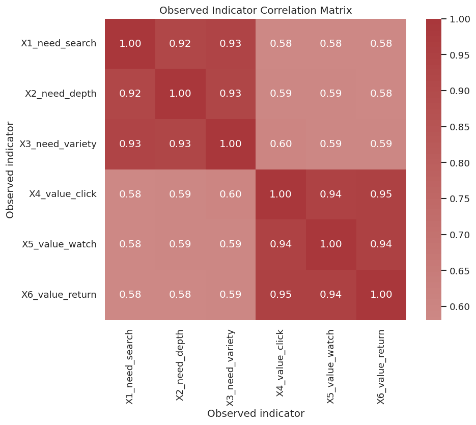
Correlation Structure Of Indicators

If the measurement model is clean, indicators of the same latent variable should be strongly correlated with each other. Indicators across different latent variables can also be correlated because the latent variables are causally connected.

indicator_correlation = observed_df.corr()
indicator_correlation.to_csv(TABLE_DIR / f"{NOTEBOOK_PREFIX}_indicator_correlation.csv")

fig, ax = plt.subplots(figsize=(8.5, 7))
sns.heatmap(indicator_correlation, cmap="vlag", center=0, annot=True, fmt=".2f", square=True, ax=ax)
ax.set_title("Observed Indicator Correlation Matrix")
ax.set_xlabel("Observed indicator")
ax.set_ylabel("Observed indicator")
plt.tight_layout()
fig.savefig(FIGURE_DIR / f"{NOTEBOOK_PREFIX}_indicator_correlation_heatmap.png", dpi=160, bbox_inches="tight")
plt.show()

The block pattern is visible: the first three indicators move together, and the last three indicators move together. Cross-block correlation is also present because the upstream latent factor causes the downstream latent factor.

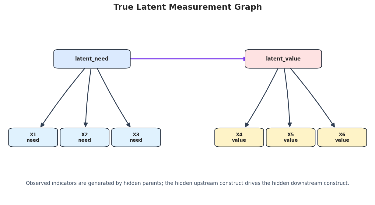
Draw The True Latent Measurement Graph

The true graph has latent variables at the top and observed indicators below. The measured columns are children of hidden parents, not peers in a simple observed-variable DAG.

def add_box(ax, xy, label, color, width=0.16, height=0.075, fontsize=10):
    x, y = xy
    patch = FancyBboxPatch(
        (x - width / 2, y - height / 2),
        width,
        height,
        boxstyle="round,pad=0.014",
        facecolor=color,
        edgecolor="#1f2937",
        linewidth=1.15,
        zorder=4,
    )
    ax.add_patch(patch)
    ax.text(x, y, label, ha="center", va="center", fontsize=fontsize, fontweight="bold", zorder=5)


def boundary_points(start, end, width=0.16, height=0.075, gap=0.012):
    x0, y0 = start
    x1, y1 = end
    dx = x1 - x0
    dy = y1 - y0
    distance = (dx**2 + dy**2) ** 0.5
    if distance == 0:
        return start, end
    ux, uy = dx / distance, dy / distance
    candidates = []
    if abs(ux) > 1e-9:
        candidates.append((width / 2) / abs(ux))
    if abs(uy) > 1e-9:
        candidates.append((height / 2) / abs(uy))
    offset = min(candidates) + gap
    return (x0 + ux * offset, y0 + uy * offset), (x1 - ux * offset, y1 - uy * offset)


def add_arrow(ax, start, end, color="#334155", rad=0.0, lw=1.7):
    start_edge, end_edge = boundary_points(start, end)
    arrow = FancyArrowPatch(
        start_edge,
        end_edge,
        arrowstyle="-|>",
        mutation_scale=17,
        linewidth=lw,
        color=color,
        connectionstyle=f"arc3,rad={rad}",
        zorder=2,
    )
    ax.add_patch(arrow)


def draw_true_measurement_graph(path):
    fig, ax = plt.subplots(figsize=(13, 6.5))
    ax.set_axis_off()
    ax.set_xlim(0, 1)
    ax.set_ylim(0, 1)

    positions = {
        "latent_need": (0.24, 0.78),
        "latent_value": (0.76, 0.78),
        "X1": (0.08, 0.35),
        "X2": (0.22, 0.35),
        "X3": (0.36, 0.35),
        "X4": (0.64, 0.35),
        "X5": (0.78, 0.35),
        "X6": (0.92, 0.35),
    }

    add_arrow(ax, positions["latent_need"], positions["latent_value"], color="#7c3aed", lw=2.0)
    for label in ["X1", "X2", "X3"]:
        add_arrow(ax, positions["latent_need"], positions[label], rad=0.03)
    for label in ["X4", "X5", "X6"]:
        add_arrow(ax, positions["latent_value"], positions[label], rad=-0.03)

    add_box(ax, positions["latent_need"], "latent_need", "#dbeafe", width=0.18)
    add_box(ax, positions["latent_value"], "latent_value", "#fee2e2", width=0.18)
    for label in ["X1", "X2", "X3"]:
        add_box(ax, positions[label], f"{label}\nneed", "#e0f2fe", width=0.105, fontsize=9.3)
    for label in ["X4", "X5", "X6"]:
        add_box(ax, positions[label], f"{label}\nvalue", "#fef3c7", width=0.105, fontsize=9.3)

    ax.text(
        0.5,
        0.10,
        "Observed indicators are generated by hidden parents; the hidden upstream construct drives the hidden downstream construct.",
        ha="center",
        va="center",
        fontsize=10,
        color="#475569",
    )
    ax.set_title("True Latent Measurement Graph", pad=18, fontsize=16, fontweight="bold")
    fig.savefig(path, dpi=160, bbox_inches="tight")
    plt.show()


draw_true_measurement_graph(FIGURE_DIR / f"{NOTEBOOK_PREFIX}_true_latent_measurement_graph.png")

This is the graph we want the GIN workflow to recover at a high level: two indicator clusters and an upstream-to-downstream latent order.

Helper Functions For GIN Output

GIN_MI returns a graph and a list of observed-index clusters. The helper functions below convert those clusters into readable tables, score cluster quality, and draw a learned measurement graph.

def observed_index_to_gin_label(index):
    return f"X{index + 1}"


def observed_index_to_name(index):
    return OBSERVED_VARIABLES[index]


def cluster_table_from_order(causal_order):
    rows = []
    for order_position, cluster in enumerate(causal_order, start=1):
        for observed_index in cluster:
            true_latent = indicator_metadata.loc[indicator_metadata["observed_index"].eq(observed_index), "true_latent"].iloc[0]
            rows.append(
                {
                    "learned_latent": f"L{order_position}",
                    "order_position": order_position,
                    "observed_index": observed_index,
                    "gin_label": observed_index_to_gin_label(observed_index),
                    "observed_variable": observed_index_to_name(observed_index),
                    "true_latent": true_latent,
                }
            )
    return pd.DataFrame(rows).sort_values(["order_position", "observed_index"]).reset_index(drop=True)


def predicted_cluster_labels(causal_order, n_observed=len(OBSERVED_VARIABLES)):
    labels = np.full(n_observed, fill_value=-1, dtype=int)
    for cluster_id, cluster in enumerate(causal_order):
        for observed_index in cluster:
            labels[observed_index] = cluster_id
    return labels


def summarize_cluster_quality(causal_order):
    table = cluster_table_from_order(causal_order)
    cluster_rows = []
    for learned_latent, group in table.groupby("learned_latent", sort=False):
        counts = group["true_latent"].value_counts()
        cluster_rows.append(
            {
                "learned_latent": learned_latent,
                "order_position": int(group["order_position"].iloc[0]),
                "members": ", ".join(group["gin_label"]),
                "member_names": ", ".join(group["observed_variable"]),
                "majority_true_latent": counts.index[0],
                "cluster_size": len(group),
                "cluster_purity": counts.iloc[0] / len(group),
            }
        )
    cluster_summary = pd.DataFrame(cluster_rows)
    ari = adjusted_rand_score(TRUE_CLUSTER_LABELS, predicted_cluster_labels(causal_order))
    majority_order = cluster_summary.sort_values("order_position")["majority_true_latent"].tolist()
    order_matches_truth = majority_order == TRUE_LATENT_ORDER
    metrics = pd.DataFrame(
        [
            {
                "n_clusters": len(cluster_summary),
                "adjusted_rand_index": ari,
                "mean_cluster_purity": cluster_summary["cluster_purity"].mean() if len(cluster_summary) else np.nan,
                "order_matches_truth": order_matches_truth,
                "learned_majority_order": " -> ".join(majority_order),
            }
        ]
    )
    return table, cluster_summary, metrics


def graph_edges_to_table(graph, method):
    return pd.DataFrame({"method": method, "edge": [str(edge) for edge in graph.get_graph_edges()]})

The adjusted Rand index scores cluster agreement without caring about the arbitrary latent labels. The order check is separate because a method can recover the right clusters but still reverse the latent order.

Run GIN-MI

GIN_MI is the mutual-information-style variant exposed in causal-learn. It is fast on this small dataset and usually recovers the two indicator groups cleanly.

start_time = time.perf_counter()
gin_mi_graph, gin_mi_order = GIN_MI(observed_df.to_numpy())
gin_mi_elapsed = time.perf_counter() - start_time

gin_mi_cluster_table, gin_mi_cluster_summary, gin_mi_metrics = summarize_cluster_quality(gin_mi_order)
gin_mi_metrics["method"] = "GIN_MI"
gin_mi_metrics["elapsed_seconds"] = gin_mi_elapsed

gin_mi_edges = graph_edges_to_table(gin_mi_graph, "GIN_MI")

gin_mi_cluster_table.to_csv(TABLE_DIR / f"{NOTEBOOK_PREFIX}_gin_mi_cluster_assignments.csv", index=False)
gin_mi_cluster_summary.to_csv(TABLE_DIR / f"{NOTEBOOK_PREFIX}_gin_mi_cluster_summary.csv", index=False)
gin_mi_metrics.to_csv(TABLE_DIR / f"{NOTEBOOK_PREFIX}_gin_mi_metrics.csv", index=False)
gin_mi_edges.to_csv(TABLE_DIR / f"{NOTEBOOK_PREFIX}_gin_mi_graph_edges.csv", index=False)

display(gin_mi_cluster_table)
display(gin_mi_cluster_summary)
display(gin_mi_metrics.round(4))
display(gin_mi_edges)

	learned_latent	order_position	observed_index	gin_label	observed_variable	true_latent
0	L1	1	0	X1	X1_need_search	latent_need
1	L1	1	1	X2	X2_need_depth	latent_need
2	L1	1	2	X3	X3_need_variety	latent_need
3	L2	2	3	X4	X4_value_click	latent_value
4	L2	2	4	X5	X5_value_watch	latent_value
5	L2	2	5	X6	X6_value_return	latent_value

	learned_latent	order_position	members	member_names	majority_true_latent	cluster_size	cluster_purity
0	L1	1	X1, X2, X3	X1_need_search, X2_need_depth, X3_need_variety	latent_need	3	1.0
1	L2	2	X4, X5, X6	X4_value_click, X5_value_watch, X6_value_return	latent_value	3	1.0

	n_clusters	adjusted_rand_index	mean_cluster_purity	order_matches_truth	learned_majority_order	method	elapsed_seconds
0	2	1.0	1.0	True	latent_need -> latent_value	GIN_MI	0.5371

	method	edge
0	GIN_MI	L1 --> X1
1	GIN_MI	L1 --> X2
2	GIN_MI	L1 --> X3
3	GIN_MI	L1 --> L2
4	GIN_MI	L2 --> X4
5	GIN_MI	L2 --> X5
6	GIN_MI	L2 --> X6

The baseline run recovers the two indicator clusters and the expected latent order. The discovered latent labels are arbitrary, but the member indicators make the learned constructs readable.

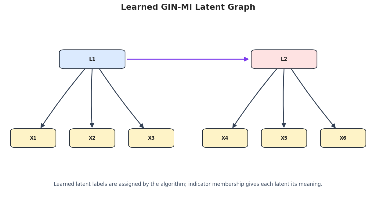
Draw The Learned GIN-MI Measurement Graph

This drawing uses the learned clusters rather than the simulator’s latent labels. The top labels L1, L2, and so on come from the learned order returned by GIN-MI.

def draw_learned_gin_graph(cluster_summary, path, title="Learned GIN-MI Latent Graph"):
    fig, ax = plt.subplots(figsize=(13, 6.5))
    ax.set_axis_off()
    ax.set_xlim(0, 1)
    ax.set_ylim(0, 1)

    cluster_summary = cluster_summary.sort_values("order_position").reset_index(drop=True)
    n_clusters = len(cluster_summary)
    latent_x = np.linspace(0.24, 0.76, n_clusters) if n_clusters > 1 else np.array([0.50])
    latent_positions = {}
    observed_positions = {}

    for i, row in cluster_summary.iterrows():
        latent = row["learned_latent"]
        x_center = latent_x[i]
        latent_positions[latent] = (x_center, 0.78)
        members = row["members"].split(", ")
        offsets = np.linspace(-0.16, 0.16, len(members)) if len(members) > 1 else np.array([0.0])
        for member, offset in zip(members, offsets):
            observed_positions[member] = (x_center + offset, 0.35)

    ordered_latents = cluster_summary["learned_latent"].tolist()
    for left, right in zip(ordered_latents[:-1], ordered_latents[1:]):
        add_arrow(ax, latent_positions[left], latent_positions[right], color="#7c3aed", lw=2.0)

    for latent in ordered_latents:
        member_labels = cluster_summary.loc[cluster_summary["learned_latent"].eq(latent), "members"].iloc[0].split(", ")
        for member in member_labels:
            add_arrow(ax, latent_positions[latent], observed_positions[member], rad=0.03)

    palette = ["#dbeafe", "#fee2e2", "#dcfce7", "#ede9fe"]
    for i, latent in enumerate(ordered_latents):
        add_box(ax, latent_positions[latent], latent, palette[i % len(palette)], width=0.15)
    for member, xy in observed_positions.items():
        add_box(ax, xy, member, "#fef3c7", width=0.095, fontsize=9.3)

    ax.text(
        0.5,
        0.10,
        "Learned latent labels are assigned by the algorithm; indicator membership gives each latent its meaning.",
        ha="center",
        va="center",
        fontsize=10,
        color="#475569",
    )
    ax.set_title(title, pad=18, fontsize=16, fontweight="bold")
    fig.savefig(path, dpi=160, bbox_inches="tight")
    plt.show()


draw_learned_gin_graph(gin_mi_cluster_summary, FIGURE_DIR / f"{NOTEBOOK_PREFIX}_gin_mi_learned_graph.png")

The learned graph has the same high-level shape as the true graph: one latent group for the first three indicators and one latent group for the last three indicators.

Compare With The Independence-Test GIN Variant

causal-learn also exposes GIN, which can use hsic or kci independence testing. On small examples, this version can be more conservative about which indicators it assigns to a cluster. We run the hsic option here because it is quick enough for a tutorial notebook.

start_time = time.perf_counter()
gin_hsic_graph, gin_hsic_order = GIN(observed_df.to_numpy(), indep_test_method="hsic", alpha=0.05)
gin_hsic_elapsed = time.perf_counter() - start_time

gin_hsic_cluster_table, gin_hsic_cluster_summary, gin_hsic_metrics = summarize_cluster_quality(gin_hsic_order)
gin_hsic_metrics["method"] = "GIN_hsic"
gin_hsic_metrics["elapsed_seconds"] = gin_hsic_elapsed

gin_hsic_edges = graph_edges_to_table(gin_hsic_graph, "GIN_hsic")

gin_hsic_cluster_table.to_csv(TABLE_DIR / f"{NOTEBOOK_PREFIX}_gin_hsic_cluster_assignments.csv", index=False)
gin_hsic_cluster_summary.to_csv(TABLE_DIR / f"{NOTEBOOK_PREFIX}_gin_hsic_cluster_summary.csv", index=False)
gin_hsic_metrics.to_csv(TABLE_DIR / f"{NOTEBOOK_PREFIX}_gin_hsic_metrics.csv", index=False)
gin_hsic_edges.to_csv(TABLE_DIR / f"{NOTEBOOK_PREFIX}_gin_hsic_graph_edges.csv", index=False)

display(gin_hsic_cluster_table)
display(gin_hsic_cluster_summary)
display(gin_hsic_metrics.round(4))
display(gin_hsic_edges)

	learned_latent	order_position	observed_index	gin_label	observed_variable	true_latent
0	L1	1	0	X1	X1_need_search	latent_need
1	L1	1	1	X2	X2_need_depth	latent_need
2	L1	1	2	X3	X3_need_variety	latent_need
3	L1	1	3	X4	X4_value_click	latent_value
4	L1	1	5	X6	X6_value_return	latent_value

	learned_latent	order_position	members	member_names	majority_true_latent	cluster_size	cluster_purity
0	L1	1	X1, X2, X3, X4, X6	X1_need_search, X2_need_depth, X3_need_variety...	latent_need	5	0.6

	n_clusters	adjusted_rand_index	mean_cluster_purity	order_matches_truth	learned_majority_order	method	elapsed_seconds
0	1	0.0	0.6	False	latent_need	GIN_hsic	0.8384

	method	edge
0	GIN_hsic	L1 --> X1
1	GIN_hsic	L1 --> X2
2	GIN_hsic	L1 --> X3
3	GIN_hsic	L1 --> X4
4	GIN_hsic	L1 --> X6

The HSIC-based run may assign fewer indicators than GIN-MI on this finite sample. That is a useful reminder that algorithm settings and independence tests affect the recovered measurement structure.

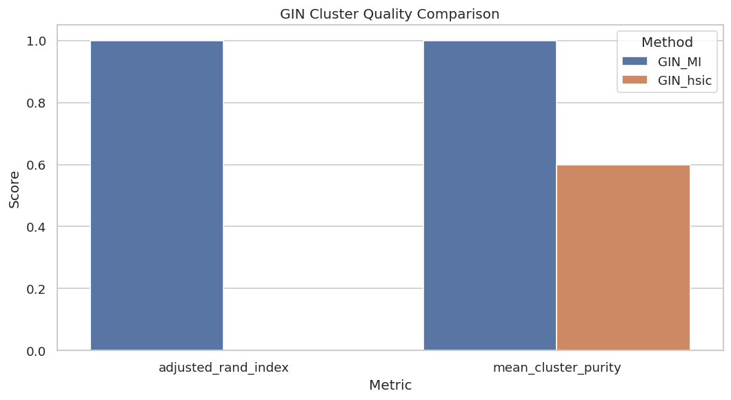
Method Comparison Table

The next table compares GIN-MI and HSIC-based GIN using cluster quality, latent order agreement, and runtime.

method_comparison = pd.concat([gin_mi_metrics, gin_hsic_metrics], ignore_index=True)
method_comparison = method_comparison[
    ["method", "n_clusters", "adjusted_rand_index", "mean_cluster_purity", "order_matches_truth", "learned_majority_order", "elapsed_seconds"]
]
method_comparison.to_csv(TABLE_DIR / f"{NOTEBOOK_PREFIX}_method_comparison.csv", index=False)
display(method_comparison.round(4))

	method	n_clusters	adjusted_rand_index	mean_cluster_purity	order_matches_truth	learned_majority_order	elapsed_seconds
0	GIN_MI	2	1.0	1.0	True	latent_need -> latent_value	0.5371
1	GIN_hsic	1	0.0	0.6	False	latent_need	0.8384

This comparison separates cluster recovery from causal order recovery. In latent discovery, both pieces matter, and either one can become unstable.

Plot Method Comparison

A simple bar plot helps compare cluster quality across the two GIN variants.

method_plot = method_comparison.melt(
    id_vars="method",
    value_vars=["adjusted_rand_index", "mean_cluster_purity"],
    var_name="metric",
    value_name="score",
)

fig, ax = plt.subplots(figsize=(9, 5))
sns.barplot(data=method_plot, x="metric", y="score", hue="method", ax=ax)
ax.set_title("GIN Cluster Quality Comparison")
ax.set_xlabel("Metric")
ax.set_ylabel("Score")
ax.set_ylim(0, 1.05)
ax.legend(title="Method")
plt.tight_layout()
fig.savefig(FIGURE_DIR / f"{NOTEBOOK_PREFIX}_method_comparison.png", dpi=160, bbox_inches="tight")
plt.show()

GIN-MI is the cleaner baseline for this notebook. The HSIC version is still useful to show how a stricter independence-testing route can behave differently.

Sensitivity To Sample Size And Measurement Noise

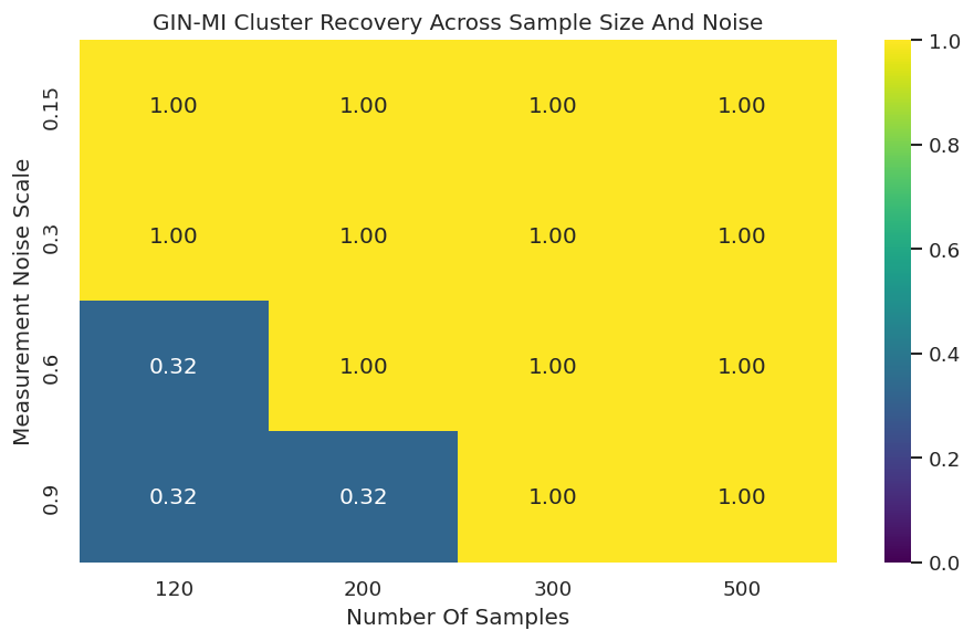
Latent cluster recovery depends on having enough observations and strong enough indicators. We scan sample size and measurement noise to see when the recovered clusters remain stable.

sensitivity_rows = []
for n_samples in [120, 200, 300, 500]:
    for measurement_noise in [0.15, 0.30, 0.60, 0.90]:
        candidate_df, _, _ = simulate_latent_indicator_data(
            n_samples=n_samples,
            seed=RANDOM_SEED,
            measurement_noise=measurement_noise,
        )
        start_time = time.perf_counter()
        _, candidate_order = GIN_MI(candidate_df.to_numpy())
        elapsed = time.perf_counter() - start_time
        _, _, metrics = summarize_cluster_quality(candidate_order)
        row = metrics.iloc[0].to_dict()
        row.update(
            {
                "n_samples": n_samples,
                "measurement_noise": measurement_noise,
                "elapsed_seconds": elapsed,
            }
        )
        sensitivity_rows.append(row)

noise_sensitivity = pd.DataFrame(sensitivity_rows)
noise_sensitivity.to_csv(TABLE_DIR / f"{NOTEBOOK_PREFIX}_sample_noise_sensitivity.csv", index=False)
display(noise_sensitivity[["n_samples", "measurement_noise", "n_clusters", "adjusted_rand_index", "mean_cluster_purity", "order_matches_truth", "elapsed_seconds"]].round(4))

	n_samples	measurement_noise	n_clusters	adjusted_rand_index	mean_cluster_purity	order_matches_truth	elapsed_seconds
0	120	0.15	2	1.0000	1.000	True	0.0461
1	120	0.30	2	1.0000	1.000	True	0.0524
2	120	0.60	2	0.3243	0.875	True	0.0489
3	120	0.90	2	0.3243	0.875	True	0.0407
4	200	0.15	2	1.0000	1.000	True	0.0812
5	200	0.30	2	1.0000	1.000	False	0.0891
6	200	0.60	2	1.0000	1.000	False	0.0840
7	200	0.90	2	0.3243	0.875	True	0.0810
8	300	0.15	2	1.0000	1.000	True	0.2057
9	300	0.30	2	1.0000	1.000	True	0.2056
10	300	0.60	2	1.0000	1.000	True	0.1998
11	300	0.90	2	1.0000	1.000	True	0.2037
12	500	0.15	2	1.0000	1.000	True	0.4466
13	500	0.30	2	1.0000	1.000	True	0.3664
14	500	0.60	2	1.0000	1.000	True	0.3637
15	500	0.90	2	1.0000	1.000	True	0.3533

The grid shows the main practical pattern: with more observations, the correct indicator clusters are more robust to noisy measurement. With very small samples and high noise, clusters can mix indicators from different latent parents.

Plot Sample And Noise Sensitivity

The heatmap shows adjusted Rand index across the sample-size and noise grid. Values near one mean the recovered indicator clusters match the true groups.

ari_heatmap = noise_sensitivity.pivot(index="measurement_noise", columns="n_samples", values="adjusted_rand_index")

fig, ax = plt.subplots(figsize=(8, 5))
sns.heatmap(ari_heatmap, annot=True, fmt=".2f", cmap="viridis", vmin=0, vmax=1, ax=ax)
ax.set_title("GIN-MI Cluster Recovery Across Sample Size And Noise")
ax.set_xlabel("Number Of Samples")
ax.set_ylabel("Measurement Noise Scale")
plt.tight_layout()
fig.savefig(FIGURE_DIR / f"{NOTEBOOK_PREFIX}_sample_noise_sensitivity.png", dpi=160, bbox_inches="tight")
plt.show()

The heatmap makes the failure region easy to see. A latent discovery report should include this kind of stress check whenever the strength of the indicators is uncertain.

Sensitivity To Non-Gaussian Assumptions

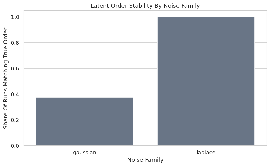
GIN is motivated by linear non-Gaussian latent-variable structure. The next cell compares Laplace and Gaussian noise across several random seeds. Cluster recovery can still look good under Gaussian noise in this simple example, but the latent order becomes less stable.

noise_family_rows = []
for distribution in ["laplace", "gaussian"]:
    for seed in range(8):
        candidate_df, _, _ = simulate_latent_indicator_data(
            n_samples=300,
            seed=seed,
            measurement_noise=0.25,
            latent_noise_distribution=distribution,
        )
        start_time = time.perf_counter()
        _, candidate_order = GIN_MI(candidate_df.to_numpy())
        elapsed = time.perf_counter() - start_time
        _, _, metrics = summarize_cluster_quality(candidate_order)
        row = metrics.iloc[0].to_dict()
        row.update({"noise_family": distribution, "seed": seed, "elapsed_seconds": elapsed})
        noise_family_rows.append(row)

noise_family_sensitivity = pd.DataFrame(noise_family_rows)
noise_family_sensitivity.to_csv(TABLE_DIR / f"{NOTEBOOK_PREFIX}_noise_family_sensitivity.csv", index=False)
display(noise_family_sensitivity[["noise_family", "seed", "adjusted_rand_index", "mean_cluster_purity", "order_matches_truth", "learned_majority_order", "elapsed_seconds"]].round(4))

	noise_family	seed	adjusted_rand_index	mean_cluster_purity	order_matches_truth	learned_majority_order	elapsed_seconds
0	laplace	0	1.0	1.0	True	latent_need -> latent_value	0.1601
1	laplace	1	1.0	1.0	True	latent_need -> latent_value	0.1729
2	laplace	2	1.0	1.0	True	latent_need -> latent_value	0.1832
3	laplace	3	1.0	1.0	True	latent_need -> latent_value	0.1897
4	laplace	4	1.0	1.0	True	latent_need -> latent_value	0.1940
5	laplace	5	1.0	1.0	True	latent_need -> latent_value	0.1918
6	laplace	6	1.0	1.0	True	latent_need -> latent_value	0.2077
7	laplace	7	1.0	1.0	True	latent_need -> latent_value	0.2031
8	gaussian	0	1.0	1.0	True	latent_need -> latent_value	0.1896
9	gaussian	1	1.0	1.0	True	latent_need -> latent_value	0.1915
10	gaussian	2	1.0	1.0	False	latent_value -> latent_need	0.1952
11	gaussian	3	1.0	1.0	False	latent_value -> latent_need	0.2099
12	gaussian	4	1.0	1.0	False	latent_value -> latent_need	0.1937
13	gaussian	5	1.0	1.0	False	latent_value -> latent_need	0.1978
14	gaussian	6	1.0	1.0	True	latent_need -> latent_value	0.2007
15	gaussian	7	1.0	1.0	False	latent_value -> latent_need	0.2042

This table separates two outcomes. The indicator clusters can remain correct while the latent order flips across seeds, especially when the distributional assumptions are weakened.

Plot Latent Order Stability

The next plot counts how often the learned majority order matches the true latent order for each noise family.

order_stability = noise_family_sensitivity.groupby("noise_family", as_index=False).agg(
    runs=("seed", "count"),
    ari_mean=("adjusted_rand_index", "mean"),
    order_match_rate=("order_matches_truth", "mean"),
)
order_stability.to_csv(TABLE_DIR / f"{NOTEBOOK_PREFIX}_noise_family_order_stability.csv", index=False)

fig, ax = plt.subplots(figsize=(8, 5))
sns.barplot(data=order_stability, x="noise_family", y="order_match_rate", color="#64748b", ax=ax)
ax.set_title("Latent Order Stability By Noise Family")
ax.set_xlabel("Noise Family")
ax.set_ylabel("Share Of Runs Matching True Order")
ax.set_ylim(0, 1.05)
plt.tight_layout()
fig.savefig(FIGURE_DIR / f"{NOTEBOOK_PREFIX}_noise_family_order_stability.png", dpi=160, bbox_inches="tight")
plt.show()

display(order_stability.round(4))

	noise_family	runs	ari_mean	order_match_rate
0	gaussian	8	1.0	0.375
1	laplace	8	1.0	1.000

The plot shows why cluster recovery and latent order recovery should be reported separately. A clean clustering result does not automatically make the direction among latent constructs stable.

Cross-Loading Stress Test

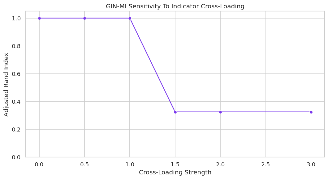
A clean measurement model says each indicator belongs to one latent parent. Real indicators often cross-load: one observed variable partly measures more than one hidden construct. The next test gradually contaminates one downstream indicator with the upstream latent factor.

cross_loading_rows = []
for cross_loading_strength in [0.0, 0.5, 1.0, 1.5, 2.0, 3.0]:
    candidate_df, _, loading_info = simulate_latent_indicator_data(
        n_samples=300,
        seed=RANDOM_SEED,
        measurement_noise=0.25,
        cross_loading_strength=cross_loading_strength,
    )
    start_time = time.perf_counter()
    _, candidate_order = GIN_MI(candidate_df.to_numpy())
    elapsed = time.perf_counter() - start_time
    cluster_table, cluster_summary, metrics = summarize_cluster_quality(candidate_order)
    row = metrics.iloc[0].to_dict()
    row.update(
        {
            "cross_loading_strength": cross_loading_strength,
            "elapsed_seconds": elapsed,
            "learned_clusters": " | ".join(cluster_summary["members"].tolist()),
        }
    )
    cross_loading_rows.append(row)

cross_loading_sensitivity = pd.DataFrame(cross_loading_rows)
cross_loading_sensitivity.to_csv(TABLE_DIR / f"{NOTEBOOK_PREFIX}_cross_loading_sensitivity.csv", index=False)
display(cross_loading_sensitivity[["cross_loading_strength", "n_clusters", "adjusted_rand_index", "mean_cluster_purity", "order_matches_truth", "learned_clusters"]].round(4))

	cross_loading_strength	n_clusters	adjusted_rand_index	mean_cluster_purity	order_matches_truth	learned_clusters
0	0.0	2	1.0000	1.000	True	X1, X2, X3 | X4, X5, X6
1	0.5	2	1.0000	1.000	True	X1, X2, X3 | X4, X5, X6
2	1.0	2	1.0000	1.000	True	X1, X2, X3 | X4, X5, X6
3	1.5	2	0.3243	0.875	True	X1, X2, X3, X6 | X4, X5
4	2.0	2	0.3243	0.875	True	X1, X2, X3, X6 | X4, X5
5	3.0	2	0.3243	0.875	True	X1, X2, X3, X6 | X4, X5

Once the cross-loading becomes large, the contaminated indicator moves into the wrong learned cluster. This is a useful failure mode because it matches a common real-data problem: proxy variables often measure multiple constructs.

Plot Cross-Loading Sensitivity

The plot shows how cluster quality changes as one indicator becomes less clean.

fig, ax = plt.subplots(figsize=(9, 5))
sns.lineplot(
    data=cross_loading_sensitivity,
    x="cross_loading_strength",
    y="adjusted_rand_index",
    marker="o",
    color="#7c3aed",
    ax=ax,
)
ax.set_title("GIN-MI Sensitivity To Indicator Cross-Loading")
ax.set_xlabel("Cross-Loading Strength")
ax.set_ylabel("Adjusted Rand Index")
ax.set_ylim(0, 1.05)
plt.tight_layout()
fig.savefig(FIGURE_DIR / f"{NOTEBOOK_PREFIX}_cross_loading_sensitivity.png", dpi=160, bbox_inches="tight")
plt.show()

The decline marks the point where the clean single-parent measurement assumption is no longer a good description of the observed indicators.

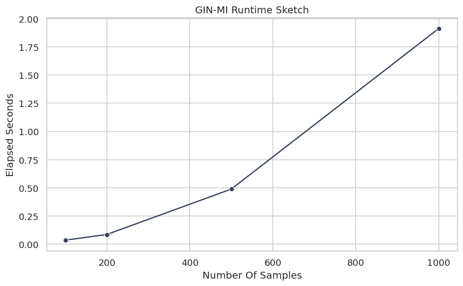
Runtime Sketch

GIN-MI is fast on six observed variables, but runtime still grows with sample size and the number of observed indicators. This small benchmark varies the sample size for the baseline six-indicator model.

runtime_rows = []
for n_samples in [100, 200, 500, 1_000]:
    candidate_df, _, _ = simulate_latent_indicator_data(n_samples=n_samples, seed=RANDOM_SEED)
    start_time = time.perf_counter()
    GIN_MI(candidate_df.to_numpy())
    elapsed = time.perf_counter() - start_time
    runtime_rows.append({"n_samples": n_samples, "n_observed_variables": len(OBSERVED_VARIABLES), "elapsed_seconds": elapsed})

runtime_table = pd.DataFrame(runtime_rows)
runtime_table.to_csv(TABLE_DIR / f"{NOTEBOOK_PREFIX}_runtime_sketch.csv", index=False)
display(runtime_table.round(4))

	n_samples	n_observed_variables	elapsed_seconds
0	100	6	0.0366
1	200	6	0.0869
2	500	6	0.4894
3	1000	6	1.9133

This is a local runtime sketch, not a universal benchmark. It does show why the tutorial keeps the sensitivity grid small.

Plot Runtime Sketch

The line plot gives a quick sense of the local cost as the number of rows increases.

fig, ax = plt.subplots(figsize=(8, 5))
sns.lineplot(data=runtime_table, x="n_samples", y="elapsed_seconds", marker="o", color="#334155", ax=ax)
ax.set_title("GIN-MI Runtime Sketch")
ax.set_xlabel("Number Of Samples")
ax.set_ylabel("Elapsed Seconds")
plt.tight_layout()
fig.savefig(FIGURE_DIR / f"{NOTEBOOK_PREFIX}_runtime_sketch.png", dpi=160, bbox_inches="tight")
plt.show()

The runtime remains manageable here. With many observed variables, the cluster search can become the expensive part.

Practical Reporting Checklist

A GIN analysis should report the measurement assumptions as clearly as the graph output. The next checklist records what a reader needs to know before trusting a latent discovery result.

reporting_checklist = pd.DataFrame(
    [
        {
            "item": "Observed indicator map",
            "what_to_report": "Which measured columns are candidate indicators and how they were selected.",
            "why_it_matters": "GIN learns latent groups from observed indicators; irrelevant columns can distort clusters.",
        },
        {
            "item": "Measurement model assumption",
            "what_to_report": "Whether indicators are expected to have one latent parent or possible cross-loadings.",
            "why_it_matters": "Cross-loaded indicators can move into the wrong learned cluster.",
        },
        {
            "item": "Distributional assumption",
            "what_to_report": "Whether non-Gaussianity is plausible or checked.",
            "why_it_matters": "The method is designed for linear non-Gaussian latent-variable structure.",
        },
        {
            "item": "Cluster quality diagnostics",
            "what_to_report": "Cluster membership, cluster size, stability, and domain meaning.",
            "why_it_matters": "The latent labels are arbitrary until the indicator membership gives them meaning.",
        },
        {
            "item": "Latent order stability",
            "what_to_report": "Whether the learned order changes across seeds, samples, or plausible preprocessing choices.",
            "why_it_matters": "Correct clusters do not guarantee a stable causal order among latent constructs.",
        },
        {
            "item": "Sensitivity checks",
            "what_to_report": "Noise, weak indicators, cross-loading, alternative tests, and sample-size checks.",
            "why_it_matters": "Latent discovery can look clean in one specification and fragile in another.",
        },
        {
            "item": "Claim strength",
            "what_to_report": "Whether the output is used as a candidate measurement graph or a causal conclusion.",
            "why_it_matters": "Latent-variable discovery needs external support before strong claims are made.",
        },
    ]
)
reporting_checklist.to_csv(TABLE_DIR / f"{NOTEBOOK_PREFIX}_reporting_checklist.csv", index=False)
display(reporting_checklist)

	item	what_to_report	why_it_matters
0	Observed indicator map	Which measured columns are candidate indicator...	GIN learns latent groups from observed indicat...
1	Measurement model assumption	Whether indicators are expected to have one la...	Cross-loaded indicators can move into the wron...
2	Distributional assumption	Whether non-Gaussianity is plausible or checked.	The method is designed for linear non-Gaussian...
3	Cluster quality diagnostics	Cluster membership, cluster size, stability, a...	The latent labels are arbitrary until the indi...
4	Latent order stability	Whether the learned order changes across seeds...	Correct clusters do not guarantee a stable cau...
5	Sensitivity checks	Noise, weak indicators, cross-loading, alterna...	Latent discovery can look clean in one specifi...
6	Claim strength	Whether the output is used as a candidate meas...	Latent-variable discovery needs external suppo...

The checklist is intentionally conservative. GIN can be a powerful way to reason about hidden constructs, but the assumptions must travel with the result.

Artifact Manifest

The final cell lists the datasets, tables, and figures created by this notebook.

artifact_paths = sorted(
    list(DATASET_DIR.glob(f"{NOTEBOOK_PREFIX}_*"))
    + list(TABLE_DIR.glob(f"{NOTEBOOK_PREFIX}_*"))
    + list(FIGURE_DIR.glob(f"{NOTEBOOK_PREFIX}_*"))
    + list(REPORT_DIR.glob(f"{NOTEBOOK_PREFIX}_*"))
)
artifact_manifest = pd.DataFrame(
    [
        {
            "artifact_type": path.parent.name,
            "path": str(path.relative_to(OUTPUT_DIR)),
            "size_kb": round(path.stat().st_size / 1024, 2),
        }
        for path in artifact_paths
    ]
)
artifact_manifest.to_csv(TABLE_DIR / f"{NOTEBOOK_PREFIX}_artifact_manifest.csv", index=False)
display(artifact_manifest)

	artifact_type	path	size_kb
0	datasets	datasets/14_synthetic_latent_truth.csv	19.14
1	datasets	datasets/14_synthetic_observed_indicators.csv	57.78
2	figures	figures/14_cross_loading_sensitivity.png	49.15
3	figures	figures/14_gin_mi_learned_graph.png	72.15
4	figures	figures/14_indicator_correlation_heatmap.png	130.90
5	figures	figures/14_method_comparison.png	41.91
6	figures	figures/14_noise_family_order_stability.png	41.83
7	figures	figures/14_runtime_sketch.png	58.17
8	figures	figures/14_sample_noise_sensitivity.png	58.83
9	figures	figures/14_true_latent_measurement_graph.png	84.37
10	tables	tables/14_artifact_manifest.csv	1.48
11	tables	tables/14_cross_loading_sensitivity.csv	0.74
12	tables	tables/14_data_audit.csv	0.61
13	tables	tables/14_gin_hsic_cluster_assignments.csv	0.27
14	tables	tables/14_gin_hsic_cluster_summary.csv	0.22
15	tables	tables/14_gin_hsic_graph_edges.csv	0.10
16	tables	tables/14_gin_hsic_metrics.csv	0.17
17	tables	tables/14_gin_mi_cluster_assignments.csv	0.30
18	tables	tables/14_gin_mi_cluster_summary.csv	0.27
19	tables	tables/14_gin_mi_graph_edges.csv	0.13
20	tables	tables/14_gin_mi_metrics.csv	0.18
21	tables	tables/14_indicator_correlation.csv	0.76
22	tables	tables/14_indicator_metadata.csv	0.25
23	tables	tables/14_method_comparison.csv	0.24
24	tables	tables/14_noise_family_order_stability.csv	0.08
25	tables	tables/14_noise_family_sensitivity.csv	1.27
26	tables	tables/14_package_versions.csv	0.08
27	tables	tables/14_reporting_checklist.csv	1.26
28	tables	tables/14_runtime_sketch.csv	0.15
29	tables	tables/14_sample_noise_sensitivity.csv	1.30
30	tables	tables/14_true_indicator_loadings.csv	0.31

The notebook leaves us with a reusable pattern: define candidate indicators, learn latent clusters, score or audit cluster quality, then stress-test the measurement assumptions before treating the latent graph as more than a hypothesis.