12: Permutation-Based Methods: GRaSP and BOSS

Permutation-based causal discovery searches over variable orderings. Once an order is proposed, each variable can only choose parents that appear earlier in that order. This turns the graph search problem into an order-search problem: find a good ordering, then infer a sparse DAG consistent with that ordering.

We introduce two causal-learn permutation-based methods:

• BOSS: Best Order Score Search.
• GRaSP: Greedy Relaxation of the Sparsest Permutation.

Both methods use local scores and order mutations to search for a graph. They are useful bridges between exact score search and scalable greedy graph search: more structured than arbitrary edge edits, but much cheaper than enumerating all DAGs.

Expected runtime: usually under 1 minute on this example dataset. The stability loops run multiple random starts, but each run is small and fast.

Learning Goals

By the end, you should be able to:

• Explain why variable orderings are useful search objects for DAG discovery.
• Understand how a fixed order restricts possible parent sets.
• Run BOSS and GRaSP from causal-learn.
• Compare permutation-based output with GES and exact search on a small graph.
• Check random-start stability for order-based methods.
• Study how GRaSP depth and sample size affect graph recovery.
• Report permutation-based results without overstating what the search guarantees.

Dataset and Experiment Setup

We use synthetic graph-discovery datasets with known structural equations and known graph truth to study Permutation-Based Methods: GRaSP And BOSS. Known graph truth lets us see when an algorithm recovers edges, misses edges, or invents edges under violated assumptions.

Read each row as a draw from a structural causal system. Columns are observed variables, and in some lessons omitted latent variables, environments, time ordering, or non-Gaussian mechanisms are deliberately introduced. The experiment studies order-based search. The quality of an ordering is interpreted through recovered parent sets and stability.

The goal is to learn what each discovery method assumes and how its output should be audited.

Mathematical Foundation

Score-based discovery searches over graphs by balancing model fit and complexity. A common score has the form

\[ \operatorname{BIC}(G)=-2\ell(\widehat\theta_G;X)+\lambda\operatorname{dim}(G)\log(n). \]

Greedy methods move through graph space locally. Exact methods optimize more globally but become expensive as the number of variables grows. A high-scoring graph is an estimated model under a score, and its causal interpretation depends on assumptions and diagnostics.

We start with order-search theory, then set up the environment and load the same linear Gaussian example dataset used by the GES and exact-search lessons. After that we show what a fixed order implies, run BOSS and GRaSP, compare them with GES and exact search, and stress-test stability across seeds, GRaSP depths, and sample sizes.

The lesson uses the linear Gaussian dataset because the permutation methods here use BIC-style local scores. That keeps the score assumptions aligned with the data-generating mechanism.

Tutorial Workflow

Permutation-Based Discovery Theory

A DAG always has at least one topological order: an ordering of variables where every parent appears before its children. If we know the correct order, the graph search becomes much easier. For each variable, we only need to decide which earlier variables are its parents.

For example, suppose the order is:

need, intent, match, engagement, renewal, support

Then match may choose parents from need and intent, but it cannot choose renewal as a parent because renewal appears later. The order itself forbids backward edges.

Permutation-based algorithms exploit this fact. They search over orders and use local scores to decide which parents are useful within each order.

From Orders to Parent Sets

For a fixed order, the best parent set for each node can be scored locally. With a decomposable score, the total graph score is:

\[ S(G) = \sum_i S_i(\mathrm{Pa}(X_i)) \]

The local score for X_i only depends on the parent set of X_i. Under an order, the candidate parent set must be a subset of variables that appear before X_i.

This is the key computational move. Instead of exploring arbitrary directed graphs, the algorithm asks: “if this order were true, which earlier variables would each node choose as parents?” Then it mutates the order to see if a better score is possible.

Sparsest Permutation Intuition

The sparsest permutation idea says that the right causal order should allow a sparse graph that explains the conditional dependence structure. If the order is wrong, the algorithm may need extra edges or awkward orientations to explain the same data.

This does not mean the sparsest graph is always the true graph. Finite samples, weak effects, hidden variables, and score mismatch can all distort sparsity. But the idea is powerful: a good order should make parent selection simple.

GRaSP searches for better permutations by relaxing and mutating orders. BOSS searches by moving variables through an order when doing so improves the score.

BOSS versus GRaSP

BOSS and GRaSP are both order-based, but they move through order space differently.

BOSS repeatedly considers moving variables to better positions in the order. After an order is updated, parent sets are recomputed from local scores. It is a greedy best-order search.

GRaSP starts with an order and uses covered-edge style relaxations, called tucks in the implementation, to improve the sparsest permutation. The depth argument controls how deep the relaxation search can go. Larger depth can escape some shallow local traps, but it can also cost more time.

Both methods can depend on random starts or random traversal choices. That is why stability across seeds is part of this lesson.

Relationship to GES and Exact Search

GES greedily edits an equivalence-class graph by adding and removing edges. Exact search optimizes the score globally over a small allowed space. BOSS and GRaSP take a third route: they search over permutations and derive parent sets consistent with those permutations.

All three families can use decomposable scores, so they can agree on friendly small problems. They can also disagree because their search paths and constraints differ.

For a small example graph, exact search is a useful benchmark. For larger graphs, permutation methods may be more practical than exact search while still giving a structured search over possible causal orderings.

What Permutation Methods Can and Cannot Claim

Permutation methods can find high-scoring DAGs and useful causal orders under score assumptions. They are especially helpful when order structure is easier to search than arbitrary graph structure.

Score optimization alone is evidence under a model. It still depends on observed variables, score choice, sample size, model class, and absence of major hidden confounding.

A careful report should include the score function, penalty, random seeds or restarts, depth settings for GRaSP, runtime, stability, and comparison to other methods.

Setup

The code below imports the scientific Python stack, BOSS, GRaSP, GES, exact BIC search, and plotting utilities. It also applies a compatibility wrapper for the BIC score used by recent NumPy versions. The wrapper preserves the same scoring formula while safely converting one-element matrix results into Python scalars.

from pathlib import Path
from importlib.metadata import PackageNotFoundError, version
import contextlib
import io
import itertools
import os
import random
import time
import warnings
# Resolve paths before importing matplotlib so the cache directory stays writable.
CWD = Path.cwd()
if CWD.name == "causal_learn" and (CWD / "outputs").exists():
    NOTEBOOK_DIR = CWD
else:
    NOTEBOOK_DIR = (CWD / "notebooks" / "tutorials" / "causal_learn").resolve()
OUTPUT_DIR = NOTEBOOK_DIR / "outputs"
DATASET_DIR = OUTPUT_DIR / "datasets"
TABLE_DIR = OUTPUT_DIR / "tables"
FIGURE_DIR = OUTPUT_DIR / "figures"
for directory in [OUTPUT_DIR, DATASET_DIR, TABLE_DIR, FIGURE_DIR, OUTPUT_DIR / "matplotlib_cache"]:
    directory.mkdir(parents=True, exist_ok=True)
os.environ.setdefault("MPLCONFIGDIR", str(OUTPUT_DIR / "matplotlib_cache"))
warnings.filterwarnings("ignore", category=FutureWarning)
warnings.filterwarnings("ignore", message="Using 'local_score_BIC_from_cov' instead for efficiency")
import numpy as np
import pandas as pd
pd.set_option("display.max_colwidth", None)
pd.set_option("display.max_columns", None)
pd.set_option("display.width", 0)
import matplotlib.pyplot as plt
import seaborn as sns
from IPython.display import display
from matplotlib.patches import FancyArrowPatch, FancyBboxPatch
import causallearn.search.PermutationBased.BOSS as boss_module
import causallearn.search.PermutationBased.GRaSP as grasp_module
import causallearn.search.ScoreBased.GES as ges_module
from causallearn.search.PermutationBased.BOSS import boss
from causallearn.search.PermutationBased.GRaSP import grasp
from causallearn.search.ScoreBased.GES import ges
from causallearn.search.ScoreBased.ExactSearch import bic_exact_search
NOTEBOOK_PREFIX = "12"
sns.set_theme(style="whitegrid", context="notebook")
plt.rcParams["figure.dpi"] = 120
plt.rcParams["savefig.facecolor"] = "white"
def local_score_BIC_from_cov(Data, i, PAi, parameters=None):
    """
    Compatibility wrapper for causal-learn BIC-from-cov scoring under recent NumPy scalar behavior.
    
    Parameters
    ----------
    Data : array-like
        Data matrix passed by causal-learn into the local score function.
    i : int
        Target variable index for the local score calculation.
    PAi : list[int]
        Parent indices proposed for the target variable in the local score.
    parameters : dict
        Score-function parameters supplied by causal-learn.
    
    Returns
    -------
    float
        BIC-style local score for one target variable and candidate parent set.
    """
    cov, n = Data
    lambda_value = 0.5 if parameters is None else parameters.get("lambda_value", 0.5)
    sigma = float(cov[i, i])
    if len(PAi) > 0:
        yX = cov[np.ix_([i], PAi)]
        XX = cov[np.ix_(PAi, PAi)]
        try:
            XX_inv = np.linalg.inv(XX)
        except np.linalg.LinAlgError:
            XX_inv = np.linalg.pinv(XX)
        sigma = float(cov[i, i] - (yX @ XX_inv @ yX.T).item())
    sigma = max(sigma, 1e-12)
    return -0.5 * n * (1 + np.log(sigma)) - lambda_value * (len(PAi) + 1) * np.log(n)
# Patch the modules that build LocalScoreClass objects during this lesson session.
boss_module.local_score_BIC_from_cov = local_score_BIC_from_cov
grasp_module.local_score_BIC_from_cov = local_score_BIC_from_cov
ges_module.local_score_BIC_from_cov = local_score_BIC_from_cov
packages = ["causal-learn", "numpy", "pandas", "matplotlib", "seaborn"]
version_rows = []
for package in packages:
    try:
        package_version = version(package)
    except PackageNotFoundError:
        package_version = "not installed"
    version_rows.append({"package": package, "version": package_version})
package_versions = pd.DataFrame(version_rows)
package_versions.to_csv(TABLE_DIR / f"{NOTEBOOK_PREFIX}_package_versions.csv", index=False)
display(package_versions)

	package	version
0	causal-learn	0.1.4.5
1	numpy	2.4.4
2	pandas	3.0.2
3	matplotlib	3.10.9
4	seaborn	0.13.2

The setup confirms the environment and patches the local score function before any permutation method is run. BOSS, GRaSP, and GES will all use the same safe BIC wrapper in this lesson.

Load the Linear Gaussian Example Data

We use the linear Gaussian dataset from the synthetic data tutorial because it matches the BIC score assumptions well. The known true graph lets us measure recovery rather than judging graphs by appearance alone.

linear_path = DATASET_DIR / "02_linear_gaussian.csv"
truth_path = TABLE_DIR / "02_base_true_dag_edges.csv"
linear_df = pd.read_csv(linear_path)
true_edges = pd.read_csv(truth_path)
VARIABLES = list(linear_df.columns)
loaded_summary = pd.DataFrame(
    [
        {
            "object": "linear Gaussian data",
            "path": str(linear_path.relative_to(NOTEBOOK_DIR)),
            "rows": len(linear_df),
            "columns": linear_df.shape[1],
        },
        {
            "object": "true edge table",
            "path": str(truth_path.relative_to(NOTEBOOK_DIR)),
            "rows": len(true_edges),
            "columns": true_edges.shape[1],
        },
    ]
)
loaded_summary.to_csv(TABLE_DIR / f"{NOTEBOOK_PREFIX}_loaded_dataset_summary.csv", index=False)
display(loaded_summary)
display(linear_df.head())
display(true_edges)

The data has six observed variables. That is small enough to compare BOSS, GRaSP, GES, and exact search directly without turning the lesson into a runtime exercise.

Helper Functions

These helpers convert causal-learn graph objects into tidy edge tables, compute recovery metrics, score fixed orders, and draw graphs in the same visual style used throughout the tutorial.

# Define reusable helpers for the Helper Functions section.
def parse_causallearn_edge(edge):
    """
    Convert a causal-learn edge object into source, endpoint pattern, and target strings.
    
    Parameters
    ----------
    edge : object
        Graph edge object or edge row being parsed, classified, or drawn.
    
    Returns
    -------
    tuple[str, str, str]
        Source node, endpoint mark, and target node parsed from a causal-learn edge.
    """
    parts = str(edge).strip().split()
    if len(parts) != 3:
        return {"source": str(edge), "edge_type": "unknown", "target": "unknown"}
    return {"source": parts[0], "edge_type": parts[1], "target": parts[2]}
def graph_to_edge_table(graph, label):
    """
    Return a tidy edge table from a causal-learn graph object.
    
    Parameters
    ----------
    graph : object
        Graph object returned by causal-learn or constructed from the edge table.
    label : str
        Readable label attached to the method, scenario, or output row.
    
    Returns
    -------
    pd.DataFrame
        Edge table with source, target, edge mark, and method metadata.
    """
    rows = [parse_causallearn_edge(edge) for edge in graph.get_graph_edges()]
    edge_df = pd.DataFrame(rows, columns=["source", "edge_type", "target"])
    if edge_df.empty:
        edge_df = pd.DataFrame(columns=["source", "edge_type", "target"])
    edge_df.insert(0, "run", label)
    return edge_df
def adjacency_to_edge_table(adjacency, variables, label):
    """
    Convert a parent-row, child-column adjacency matrix into a tidy directed edge table.
    
    Parameters
    ----------
    adjacency : object
        Adjacency matrix encoding candidate parent-child edges.
    variables : list[str]
        Variables included in the graph, lag frame, or diagnostic.
    label : str
        Readable label attached to the method, scenario, or output row.
    
    Returns
    -------
    pd.DataFrame
        Graph edge table for adjacency to edge table, including node names and edge-orientation information where available.
    """
    rows = []
    for parent_idx, child_idx in zip(*np.where(adjacency > 0)):
        rows.append(
            {
                "run": label,
                "source": variables[int(parent_idx)],
                "edge_type": "-->",
                "target": variables[int(child_idx)],
            }
        )
    return pd.DataFrame(rows, columns=["run", "source", "edge_type", "target"])
def directed_pairs(edge_df):
    """
    Extract definite directed pairs from an edge table.
    
    Parameters
    ----------
    edge_df : pd.DataFrame
        Learned or oracle edge table being summarized or drawn.
    
    Returns
    -------
    set[tuple[str, str]]
        Ordered source-target pairs representing directed learned edges.
    """
    pairs = set()
    for row in edge_df.itertuples(index=False):
        if row.edge_type == "-->":
            pairs.add((row.source, row.target))
        elif row.edge_type == "<--":
            pairs.add((row.target, row.source))
    return pairs
def skeleton_pairs(edge_df):
    """
    Extract adjacencies while ignoring direction.
    
    Parameters
    ----------
    edge_df : pd.DataFrame
        Learned or oracle edge table being summarized or drawn.
    
    Returns
    -------
    set[tuple[str, str]]
        Unordered node pairs representing the learned graph skeleton.
    """
    pairs = set()
    for row in edge_df.itertuples(index=False):
        if row.target != "unknown":
            pairs.add(frozenset([row.source, row.target]))
    return pairs
def summarize_against_truth(edge_df, truth_df, label):
    """
    Compute graph-recovery metrics against a directed truth table.
    
    Parameters
    ----------
    edge_df : pd.DataFrame
        Learned or oracle edge table being summarized or drawn.
    truth_df : pd.DataFrame
        Oracle edge table used as the synthetic ground-truth benchmark.
    label : str
        Readable label attached to the method, scenario, or output row.
    
    Returns
    -------
    pd.DataFrame
        Graph-recovery summary table with edge counts, precision, recall, missing edges, and extra edges.
    """
    true_directed = set(zip(truth_df["source"], truth_df["target"]))
    true_skeleton = {frozenset(edge) for edge in true_directed}
    learned_directed = directed_pairs(edge_df)
    learned_skeleton = skeleton_pairs(edge_df)
    correct_directed = learned_directed & true_directed
    reversed_true = {(src, dst) for src, dst in true_directed if (dst, src) in learned_directed}
    missing_skeleton = true_skeleton - learned_skeleton
    extra_skeleton = learned_skeleton - true_skeleton
    unresolved_true = 0
    for src, dst in true_directed:
        pair = frozenset([src, dst])
        if pair in learned_skeleton and (src, dst) not in learned_directed and (dst, src) not in learned_directed:
            unresolved_true += 1
    directed_count = len(learned_directed)
    return pd.DataFrame(
        [
            {
                "run": label,
                "learned_edges_total": len(edge_df),
                "definite_directed_edges": directed_count,
                "true_edges": len(true_directed),
                "correct_directed_edges": len(correct_directed),
                "directed_precision": len(correct_directed) / directed_count if directed_count else np.nan,
                "directed_recall": len(correct_directed) / len(true_directed) if true_directed else np.nan,
                "reversed_true_edges": len(reversed_true),
                "unresolved_true_adjacencies": unresolved_true,
                "missing_true_adjacencies": len(missing_skeleton),
                "extra_adjacencies": len(extra_skeleton),
            }
        ]
    )
def run_boss(data_df, label, seed=1, lambda_value=0.5):
    """
    Run BOSS with a controlled random seed.
    
    Parameters
    ----------
    data_df : pd.DataFrame
        Dataset for the current simulated or observed experiment.
    label : str
        Readable label attached to the method, scenario, or output row.
    seed : int
        Random seed for reproducible simulation or resampling.
    lambda_value : float
        Numeric value for `lambda`.
    
    Returns
    -------
    tuple
        Tuple containing graph, edge_table, elapsed.
    """
    random.seed(seed)
    np.random.seed(seed)
    start = time.perf_counter()
    buffer = io.StringIO()
    with contextlib.redirect_stdout(buffer):
        graph = boss(
            data_df.to_numpy(),
            score_func="local_score_BIC_from_cov",
            parameters={"lambda_value": lambda_value},
            verbose=False,
            node_names=list(data_df.columns),
        )
    elapsed = time.perf_counter() - start
    edge_table = graph_to_edge_table(graph, label=label)
    return graph, edge_table, elapsed
def run_grasp(data_df, label, seed=1, depth=4, lambda_value=0.5):
    """
    Run GRaSP with a controlled random seed and chosen depth.
    
    Parameters
    ----------
    data_df : pd.DataFrame
        Dataset for the current simulated or observed experiment.
    label : str
        Readable label attached to the method, scenario, or output row.
    seed : int
        Random seed for reproducible simulation or resampling.
    depth : int
        Maximum conditioning-set depth used by the discovery algorithm.
    lambda_value : float
        Numeric value for `lambda`.
    
    Returns
    -------
    tuple
        Tuple containing graph, edge_table, elapsed.
    """
    random.seed(seed)
    np.random.seed(seed)
    start = time.perf_counter()
    buffer = io.StringIO()
    with contextlib.redirect_stdout(buffer):
        graph = grasp(
            data_df.to_numpy(),
            score_func="local_score_BIC_from_cov",
            depth=depth,
            parameters={"lambda_value": lambda_value},
            verbose=False,
            node_names=list(data_df.columns),
        )
    elapsed = time.perf_counter() - start
    edge_table = graph_to_edge_table(graph, label=label)
    return graph, edge_table, elapsed
def run_ges_bic(data_df, label, lambda_value=0.5):
    """
    Run BIC-GES quietly for comparison.
    
    Parameters
    ----------
    data_df : pd.DataFrame
        Dataset for the current simulated or observed experiment.
    label : str
        Readable label attached to the method, scenario, or output row.
    lambda_value : float
        Numeric value for `lambda`.
    
    Returns
    -------
    tuple
        Tuple containing record, edge_table, elapsed.
    """
    start = time.perf_counter()
    buffer = io.StringIO()
    with contextlib.redirect_stdout(buffer):
        record = ges(
            data_df.to_numpy(),
            score_func="local_score_BIC",
            node_names=list(data_df.columns),
            lambda_value=lambda_value,
        )
    elapsed = time.perf_counter() - start
    edge_table = graph_to_edge_table(record["G"], label=label)
    return record, edge_table, elapsed
def run_exact_bic(data_df, label):
    """
    Run exact BIC search with A* for the small example graph.
    
    Parameters
    ----------
    data_df : pd.DataFrame
        Dataset for the current simulated or observed experiment.
    label : str
        Readable label attached to the method, scenario, or output row.
    
    Returns
    -------
    tuple
        Tuple containing adjacency, stats, edge_table, elapsed.
    """
    start = time.perf_counter()
    adjacency, stats = bic_exact_search(data_df.to_numpy(), search_method="astar", verbose=False)
    elapsed = time.perf_counter() - start
    edge_table = adjacency_to_edge_table(adjacency, list(data_df.columns), label=label)
    return adjacency, stats, edge_table, elapsed
def best_parent_sets_for_order(data_df, order, lambda_value=0.5, max_parents=None):
    """
    Exhaustively choose the best parent set for each node given a fixed order.
    
    Parameters
    ----------
    data_df : pd.DataFrame
        Dataset for the current simulated or observed experiment.
    order : object
        Variable ordering proposed by an order-based graph-search method.
    lambda_value : float
        Numeric value for `lambda`.
    max_parents : object
        Maximum number of candidate parents allowed in the graph search.
    
    Returns
    -------
    tuple
        Tuple containing parent_table, edge_table, total_score.
    """
    data = data_df.to_numpy()
    cov = np.cov(data.T, ddof=0)
    n = data.shape[0]
    index = {name: i for i, name in enumerate(data_df.columns)}
    rows = []
    edge_rows = []
    total_score = 0.0
    for position, child in enumerate(order):
        child_idx = index[child]
        candidate_parents = list(order[:position])
        parent_limit = len(candidate_parents) if max_parents is None else min(max_parents, len(candidate_parents))
        best_score = -np.inf
        best_parents = []
        for size in range(parent_limit + 1):
            for parent_names in itertools.combinations(candidate_parents, size):
                parent_indices = [index[name] for name in parent_names]
                score = local_score_BIC_from_cov((cov, n), child_idx, parent_indices, {"lambda_value": lambda_value})
                if score > best_score:
                    best_score = score
                    best_parents = list(parent_names)
        total_score += best_score
        rows.append(
            {
                "order_label": " -> ".join(order),
                "child": child,
                "position": position + 1,
                "allowed_parent_count": len(candidate_parents),
                "selected_parents": ", ".join(best_parents) if best_parents else "none",
                "local_score": best_score,
            }
        )
        for parent in best_parents:
            edge_rows.append({"run": "fixed_order", "source": parent, "edge_type": "-->", "target": child})
    parent_table = pd.DataFrame(rows)
    edge_table = pd.DataFrame(edge_rows, columns=["run", "source", "edge_type", "target"])
    return parent_table, edge_table, total_score
GRAPH_POSITIONS = {
    "need": (0.11, 0.72),
    "intent": (0.11, 0.28),
    "match": (0.39, 0.50),
    "engagement": (0.62, 0.50),
    "renewal": (0.89, 0.72),
    "support": (0.89, 0.28),
}
NODE_LABELS = {name: name.title() for name in GRAPH_POSITIONS}
NODE_COLORS = {
    "need": "#e0f2fe",
    "intent": "#dbeafe",
    "match": "#ecfccb",
    "engagement": "#fef3c7",
    "renewal": "#fee2e2",
    "support": "#f3e8ff",
}
def trim_edge_to_box(start, end, box_w=0.145, box_h=0.095, gap=0.012):
    """
    Return edge endpoints that stop just outside source and target boxes.
    
    Parameters
    ----------
    start : tuple[float, float]
        Starting coordinate of the arrow or edge segment.
    end : tuple[float, float]
        Ending coordinate of the arrow or edge segment.
    box_w : float
        Width of the node box used to trim edge endpoints.
    box_h : float
        Height of the node box used to trim edge endpoints.
    gap : float
        Extra spacing between an edge endpoint and a node boundary.
    
    Returns
    -------
    tuple[tuple[float, float], tuple[float, float]]
        Start and end coordinates trimmed so the edge stops at box boundaries.
    """
    x0, y0 = start
    x1, y1 = end
    dx = x1 - x0
    dy = y1 - y0
    length = float(np.hypot(dx, dy))
    if length == 0:
        return start, end
    effective_w = box_w + 0.04
    effective_h = box_h + 0.04
    x_limit = (effective_w / 2) / abs(dx) if dx else np.inf
    y_limit = (effective_h / 2) / abs(dy) if dy else np.inf
    t = min(x_limit, y_limit) + gap / length
    return (x0 + dx * t, y0 + dy * t), (x1 - dx * t, y1 - dy * t)
def draw_box_graph(edge_df, title, path, note=None):
    """
    Draw a DAG-style graph with rounded boxes and visible arrowheads.
    
    Parameters
    ----------
    edge_df : pd.DataFrame
        Learned or oracle edge table being summarized or drawn.
    title : str
        Title shown above the plot.
    path : str or pathlib.Path
        Optional output path for the figure.
    note : str or None
        Optional explanatory note shown in the plot.
    
    Returns
    -------
    None
        Draws the graph diagram directly on the Matplotlib axes and saves it when requested.
    """
    fig, ax = plt.subplots(figsize=(12, 6.2))
    ax.set_axis_off()
    ax.set_xlim(-0.02, 1.02)
    ax.set_ylim(0.04, 0.96)
    box_w, box_h = 0.145, 0.095
    for row in edge_df.itertuples(index=False):
        if row.source not in GRAPH_POSITIONS or row.target not in GRAPH_POSITIONS:
            continue
        raw_start = GRAPH_POSITIONS[row.source]
        raw_end = GRAPH_POSITIONS[row.target]
        if row.edge_type == "<--":
            raw_start, raw_end = raw_end, raw_start
        start, end = trim_edge_to_box(raw_start, raw_end, box_w=box_w, box_h=box_h)
        if row.edge_type in {"-->", "<--"}:
            arrowstyle = "-|>"
            mutation_scale = 18
            linewidth = 1.8
            color = "#334155"
        else:
            arrowstyle = "-"
            mutation_scale = 1
            linewidth = 1.5
            color = "#64748b"
        arrow = FancyArrowPatch(
            start,
            end,
            arrowstyle=arrowstyle,
            mutation_scale=mutation_scale,
            linewidth=linewidth,
            color=color,
            connectionstyle="arc3,rad=0.035",
            zorder=2,
        )
        ax.add_patch(arrow)
    for node, (x, y) in GRAPH_POSITIONS.items():
        rect = FancyBboxPatch(
            (x - box_w / 2, y - box_h / 2),
            box_w,
            box_h,
            boxstyle="round,pad=0.018",
            facecolor=NODE_COLORS[node],
            edgecolor="#1f2937",
            linewidth=1.1,
            zorder=5,
        )
        ax.add_patch(rect)
        ax.text(x, y, NODE_LABELS[node], ha="center", va="center", fontsize=10.5, fontweight="bold", zorder=6)
    if note:
        ax.text(0.50, 0.08, note, ha="center", va="center", fontsize=10, color="#475569")
    ax.set_title(title, pad=18, fontsize=14, fontweight="bold")
    fig.savefig(path, dpi=160, bbox_inches="tight")
    plt.show()
def truth_as_edge_table(truth_df, label="truth"):
    """
    Convert a truth table into a plotting-ready edge table.
    
    Parameters
    ----------
    truth_df : pd.DataFrame
        Oracle edge table used as the synthetic ground-truth benchmark.
    label : str
        Readable label attached to the method, scenario, or output row.
    
    Returns
    -------
    pd.DataFrame
        Oracle graph edge table with run label and directed-edge marks.
    """
    return truth_df.assign(run=label, edge_type="-->")[["run", "source", "edge_type", "target"]]

The helper set includes a small fixed-order scorer. That scorer is not a replacement for BOSS or GRaSP; it is a teaching device for seeing how a proposed order restricts parent choices.

Draw the True DAG

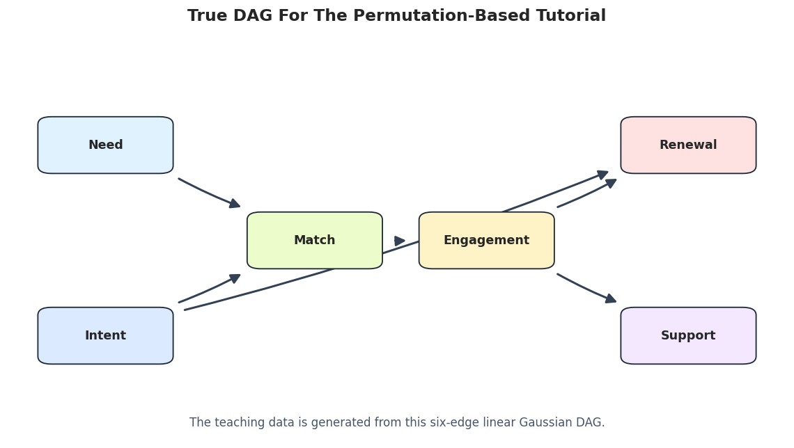
Before running order-based methods, we draw the known data-generating DAG. This is the target used in the recovery metrics.

true_plot_edges = truth_as_edge_table(true_edges)
draw_box_graph(
    true_plot_edges,
    title="True DAG For The Permutation-Based Tutorial",
    path=FIGURE_DIR / f"{NOTEBOOK_PREFIX}_true_dag.png",
    note="The example data is generated from this six-edge linear Gaussian DAG.",
)

The true graph has two root variables, a mediator chain, and two downstream outcomes. A good order should place causes before effects so parent selection can recover these edges.

Fixed-Order Parent Selection Demo

The code below shows why order matters. We compare a plausible causal order with a deliberately reversed order. For each order, the code finds the best local BIC parent set for every node using only variables that appear earlier in the order.

causal_order = ["need", "intent", "match", "engagement", "renewal", "support"]
reversed_order = list(reversed(causal_order))
fixed_order_rows = []
fixed_order_edge_tables = []
for order_name, order in [("causal_order", causal_order), ("reversed_order", reversed_order)]:
    parent_table, edge_table, total_score = best_parent_sets_for_order(
        linear_df,
        order,
        lambda_value=0.5,
        max_parents=3,
    )
    parent_table["order_name"] = order_name
    parent_table["total_order_score"] = total_score
    edge_table["run"] = order_name
    fixed_order_rows.append(parent_table)
    fixed_order_edge_tables.append(edge_table)
fixed_order_parent_sets = pd.concat(fixed_order_rows, ignore_index=True)
fixed_order_edges = pd.concat(fixed_order_edge_tables, ignore_index=True)
fixed_order_metrics = pd.concat(
    [
        summarize_against_truth(fixed_order_edges[fixed_order_edges["run"] == name], true_edges, name)
        for name in ["causal_order", "reversed_order"]
    ],
    ignore_index=True,
)
order_score_summary = fixed_order_parent_sets.groupby("order_name", as_index=False).agg(
    total_order_score=("total_order_score", "first"),
    selected_parent_links=("selected_parents", lambda values: sum(value != "none" for value in values)),
)
fixed_order_parent_sets.to_csv(TABLE_DIR / f"{NOTEBOOK_PREFIX}_fixed_order_parent_sets.csv", index=False)
fixed_order_edges.to_csv(TABLE_DIR / f"{NOTEBOOK_PREFIX}_fixed_order_edges.csv", index=False)
fixed_order_metrics.to_csv(TABLE_DIR / f"{NOTEBOOK_PREFIX}_fixed_order_metrics.csv", index=False)
order_score_summary.to_csv(TABLE_DIR / f"{NOTEBOOK_PREFIX}_fixed_order_score_summary.csv", index=False)
display(order_score_summary.round(4))
display(fixed_order_parent_sets[["order_name", "child", "position", "selected_parents", "local_score"]].round(4))
display(fixed_order_metrics.round(4))

	order_name	total_order_score	selected_parent_links
0	causal_order	-2547.9957	4
1	reversed_order	-2562.6663	5

	order_name	child	position	selected_parents	local_score
0	causal_order	need	1	none	-1253.9120
1	causal_order	intent	2	none	-1253.9120
2	causal_order	match	3	need, intent	504.3279
3	causal_order	engagement	4	match	142.9078
4	causal_order	renewal	5	intent, engagement	53.2493
5	causal_order	support	6	engagement	-740.6566
6	reversed_order	support	1	none	-1253.9120
7	reversed_order	renewal	2	support	-1058.9669
8	reversed_order	engagement	3	support, renewal	-197.2864
9	reversed_order	match	4	renewal, engagement	234.5766
10	reversed_order	intent	5	renewal, engagement, match	-137.2946
11	reversed_order	need	6	match, intent	-149.7830

	run	learned_edges_total	definite_directed_edges	true_edges	correct_directed_edges	directed_precision	directed_recall	reversed_true_edges	unresolved_true_adjacencies	missing_true_adjacencies	extra_adjacencies
0	causal_order	6	6	6	6	1.0	1.0	0	0	0	0
1	reversed_order	10	10	6	0	0.0	0.0	6	0	0	4

The causal order should score better and recover the direct structure more naturally. The reversed order may still fit dependencies, but it must explain them with backward or awkward parent choices.

Run BOSS and GRaSP

Now we run the actual permutation-based algorithms. The baseline uses the same BIC penalty as the GES comparison later and fixes the random seed so the lesson is reproducible.

BASELINE_SEED = 1
LAMBDA_VALUE = 0.5
GRASP_DEPTH = 4
boss_graph, boss_edges, boss_elapsed = run_boss(
    linear_df,
    label="BOSS",
    seed=BASELINE_SEED,
    lambda_value=LAMBDA_VALUE,
)
grasp_graph, grasp_edges, grasp_elapsed = run_grasp(
    linear_df,
    label="GRaSP_depth_4",
    seed=BASELINE_SEED,
    depth=GRASP_DEPTH,
    lambda_value=LAMBDA_VALUE,
)
permutation_edges = pd.concat([boss_edges, grasp_edges], ignore_index=True)
permutation_metrics = pd.concat(
    [
        summarize_against_truth(boss_edges, true_edges, "BOSS"),
        summarize_against_truth(grasp_edges, true_edges, "GRaSP_depth_4"),
    ],
    ignore_index=True,
)
permutation_metrics["elapsed_seconds"] = [boss_elapsed, grasp_elapsed]
permutation_metrics["seed"] = BASELINE_SEED
permutation_metrics["lambda_value"] = LAMBDA_VALUE
permutation_edges.to_csv(TABLE_DIR / f"{NOTEBOOK_PREFIX}_boss_grasp_edges.csv", index=False)
permutation_metrics.to_csv(TABLE_DIR / f"{NOTEBOOK_PREFIX}_boss_grasp_metrics.csv", index=False)
display(permutation_edges)
display(permutation_metrics.round(4))

	run	source	edge_type	target
0	BOSS	need	-->	match
1	BOSS	intent	-->	match
2	BOSS	intent	-->	renewal
3	BOSS	match	-->	engagement
4	BOSS	engagement	-->	renewal
5	BOSS	engagement	-->	support
6	GRaSP_depth_4	need	-->	match
7	GRaSP_depth_4	intent	-->	match
8	GRaSP_depth_4	intent	-->	renewal
9	GRaSP_depth_4	match	-->	engagement
10	GRaSP_depth_4	engagement	-->	renewal
11	GRaSP_depth_4	engagement	-->	support

	run	learned_edges_total	definite_directed_edges	true_edges	correct_directed_edges	directed_precision	directed_recall	reversed_true_edges	unresolved_true_adjacencies	missing_true_adjacencies	extra_adjacencies	elapsed_seconds	seed	lambda_value
0	BOSS	6	6	6	6	1.0	1.0	0	0	0	0	0.0123	1	0.5
1	GRaSP_depth_4	6	6	6	6	1.0	1.0	0	0	0	0	0.0100	1	0.5

On this friendly six-variable dataset, both methods should recover the same core graph. That is reassuring, but the stability sections below are still necessary because order-search algorithms can depend on random starts and search settings.

Draw the BOSS Graph

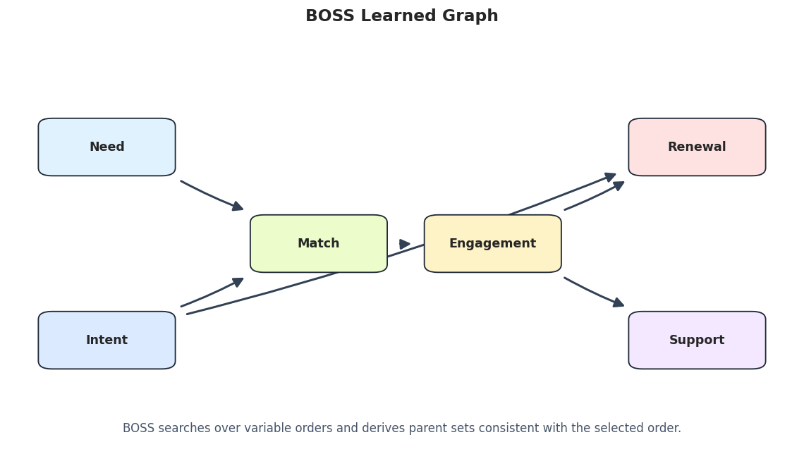
The BOSS graph is drawn first because BOSS is a clean baseline for best-order score search in this lesson.

draw_box_graph(
    boss_edges,
    title="BOSS Learned Graph",
    path=FIGURE_DIR / f"{NOTEBOOK_PREFIX}_boss_graph.png",
    note="BOSS searches over variable orders and derives parent sets consistent with the selected order.",
)

The graph layout matches the true DAG layout so differences are easy to see. For this baseline seed and dataset, the learned graph should be visually aligned with the true structure.

Diagnostics and Interpretation

Compare with GES and Exact Search

Permutation-based search is one way to optimize graph structure. To anchor the result, we compare BOSS and GRaSP with GES and exact BIC search on the same data.

ges_record, ges_edges, ges_elapsed = run_ges_bic(linear_df, label="GES_BIC", lambda_value=LAMBDA_VALUE)
exact_adjacency, exact_stats, exact_edges, exact_elapsed = run_exact_bic(linear_df, label="Exact_BIC_AStar")
method_edges = pd.concat([boss_edges, grasp_edges, ges_edges, exact_edges], ignore_index=True)
method_metrics = pd.concat(
    [
        summarize_against_truth(boss_edges, true_edges, "BOSS"),
        summarize_against_truth(grasp_edges, true_edges, "GRaSP_depth_4"),
        summarize_against_truth(ges_edges, true_edges, "GES_BIC"),
        summarize_against_truth(exact_edges, true_edges, "Exact_BIC_AStar"),
    ],
    ignore_index=True,
)
method_metrics["elapsed_seconds"] = [boss_elapsed, grasp_elapsed, ges_elapsed, exact_elapsed]
method_metrics["search_family"] = ["permutation", "permutation", "score_greedy", "score_exact"]
method_edges.to_csv(TABLE_DIR / f"{NOTEBOOK_PREFIX}_method_comparison_edges.csv", index=False)
method_metrics.to_csv(TABLE_DIR / f"{NOTEBOOK_PREFIX}_method_comparison_metrics.csv", index=False)
pd.DataFrame([exact_stats]).to_csv(TABLE_DIR / f"{NOTEBOOK_PREFIX}_exact_search_stats.csv", index=False)
display(method_edges)
display(method_metrics.round(4))

	run	source	edge_type	target
0	BOSS	need	-->	match
1	BOSS	intent	-->	match
2	BOSS	intent	-->	renewal
3	BOSS	match	-->	engagement
4	BOSS	engagement	-->	renewal
5	BOSS	engagement	-->	support
6	GRaSP_depth_4	need	-->	match
7	GRaSP_depth_4	intent	-->	match
8	GRaSP_depth_4	intent	-->	renewal
9	GRaSP_depth_4	match	-->	engagement
10	GRaSP_depth_4	engagement	-->	renewal
11	GRaSP_depth_4	engagement	-->	support
12	GES_BIC	need	-->	match
13	GES_BIC	intent	-->	match
14	GES_BIC	intent	-->	renewal
15	GES_BIC	match	-->	engagement
16	GES_BIC	engagement	-->	renewal
17	GES_BIC	engagement	-->	support
18	Exact_BIC_AStar	need	-->	match
19	Exact_BIC_AStar	intent	-->	match
20	Exact_BIC_AStar	intent	-->	renewal
21	Exact_BIC_AStar	match	-->	engagement
22	Exact_BIC_AStar	engagement	-->	renewal
23	Exact_BIC_AStar	engagement	-->	support

	run	learned_edges_total	definite_directed_edges	true_edges	correct_directed_edges	directed_precision	directed_recall	reversed_true_edges	unresolved_true_adjacencies	missing_true_adjacencies	extra_adjacencies	elapsed_seconds	search_family
0	BOSS	6	6	6	6	1.0	1.0	0	0	0	0	0.0123	permutation
1	GRaSP_depth_4	6	6	6	6	1.0	1.0	0	0	0	0	0.0100	permutation
2	GES_BIC	6	6	6	6	1.0	1.0	0	0	0	0	0.0227	score_greedy
3	Exact_BIC_AStar	6	6	6	6	1.0	1.0	0	0	0	0	0.0156	score_exact

Agreement across BOSS, GRaSP, GES, and exact search is a strong teaching result for this small aligned dataset. In real data, disagreement is often more informative than agreement because it exposes assumption and search sensitivity.

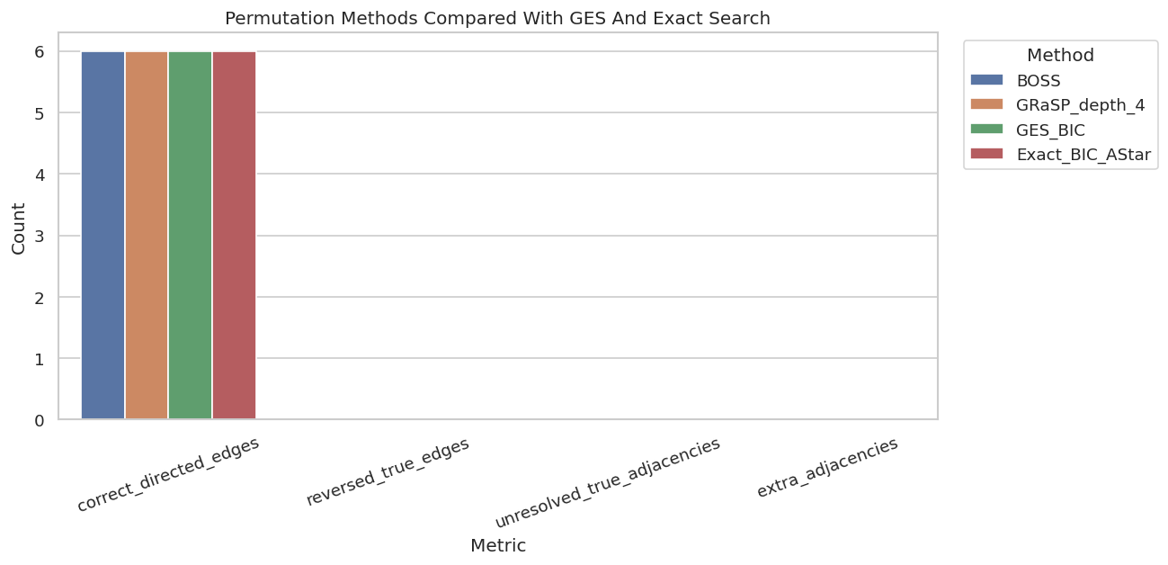
Plot Method Comparison

The table above is compact, but a plot makes recovery differences easier to scan. We focus on directed correctness, unresolved true adjacencies, and extra adjacencies.

method_plot_df = method_metrics.melt(
    id_vars=["run", "search_family"],
    value_vars=["correct_directed_edges", "reversed_true_edges", "unresolved_true_adjacencies", "extra_adjacencies"],
    var_name="metric",
    value_name="count",
)
fig, ax = plt.subplots(figsize=(11, 5.4))
sns.barplot(data=method_plot_df, x="metric", y="count", hue="run", ax=ax)
ax.set_title("Permutation Methods Compared With GES And Exact Search")
ax.set_xlabel("Metric")
ax.set_ylabel("Count")
ax.tick_params(axis="x", rotation=20)
ax.legend(title="Method", bbox_to_anchor=(1.02, 1), loc="upper left")
plt.tight_layout()
fig.savefig(FIGURE_DIR / f"{NOTEBOOK_PREFIX}_method_comparison_metrics.png", dpi=160, bbox_inches="tight")
plt.show()

The plot should show that all methods perform well in this controlled setting. The later sensitivity sections are where differences become more visible.

That makes the comparison interpretable because differences across methods can be tied to estimator behavior while preprocessing and evaluation stay fixed.

Random-Seed Stability

BOSS and GRaSP use random order traversal or random starting choices. The code below repeats each method across several seeds and records whether the recovered graph changes.

stability_rows = []
stability_edges = []
for seed in range(10):
    for method_name in ["BOSS", "GRaSP_depth_4"]:
        if method_name == "BOSS":
            _, edge_table, elapsed = run_boss(linear_df, label=f"BOSS_seed_{seed}", seed=seed, lambda_value=LAMBDA_VALUE)
        else:
            _, edge_table, elapsed = run_grasp(linear_df, label=f"GRaSP_seed_{seed}", seed=seed, depth=GRASP_DEPTH, lambda_value=LAMBDA_VALUE)
        metrics = summarize_against_truth(edge_table, true_edges, label=f"{method_name}_seed_{seed}")
        metrics["method"] = method_name
        metrics["seed"] = seed
        metrics["elapsed_seconds"] = elapsed
        edge_signature = " | ".join(sorted(f"{row.source} {row.edge_type} {row.target}" for row in edge_table.itertuples(index=False)))
        metrics["edge_signature"] = edge_signature
        stability_rows.append(metrics)
        edge_table["method"] = method_name
        edge_table["seed"] = seed
        stability_edges.append(edge_table)
seed_stability_metrics = pd.concat(stability_rows, ignore_index=True)
seed_stability_edges = pd.concat(stability_edges, ignore_index=True)
seed_stability_summary = seed_stability_metrics.groupby("method", as_index=False).agg(
    runs=("seed", "count"),
    unique_graphs=("edge_signature", "nunique"),
    mean_correct_directed_edges=("correct_directed_edges", "mean"),
    min_correct_directed_edges=("correct_directed_edges", "min"),
    max_extra_adjacencies=("extra_adjacencies", "max"),
    median_elapsed_seconds=("elapsed_seconds", "median"),
)
seed_stability_metrics.to_csv(TABLE_DIR / f"{NOTEBOOK_PREFIX}_seed_stability_metrics.csv", index=False)
seed_stability_edges.to_csv(TABLE_DIR / f"{NOTEBOOK_PREFIX}_seed_stability_edges.csv", index=False)
seed_stability_summary.to_csv(TABLE_DIR / f"{NOTEBOOK_PREFIX}_seed_stability_summary.csv", index=False)
display(seed_stability_summary.round(4))
display(seed_stability_metrics[["method", "seed", "correct_directed_edges", "unresolved_true_adjacencies", "extra_adjacencies", "elapsed_seconds"]].round(4))

	method	runs	unique_graphs	mean_correct_directed_edges	min_correct_directed_edges	max_extra_adjacencies	median_elapsed_seconds
0	BOSS	10	1	6.0	6	0	0.0090
1	GRaSP_depth_4	10	1	6.0	6	0	0.0078

	method	seed	correct_directed_edges	unresolved_true_adjacencies	extra_adjacencies	elapsed_seconds
0	BOSS	0	6	0	0	0.0099
1	GRaSP_depth_4	0	6	0	0	0.0086
2	BOSS	1	6	0	0	0.0091
3	GRaSP_depth_4	1	6	0	0	0.0074
4	BOSS	2	6	0	0	0.0088
5	GRaSP_depth_4	2	6	0	0	0.0080
6	BOSS	3	6	0	0	0.0092
7	GRaSP_depth_4	3	6	0	0	0.0060
8	BOSS	4	6	0	0	0.0088
9	GRaSP_depth_4	4	6	0	0	0.0102
10	BOSS	5	6	0	0	0.0092
11	GRaSP_depth_4	5	6	0	0	0.0061
12	BOSS	6	6	0	0	0.0090
13	GRaSP_depth_4	6	6	0	0	0.0076
14	BOSS	7	6	0	0	0.0089
15	GRaSP_depth_4	7	6	0	0	0.0091
16	BOSS	8	6	0	0	0.0089
17	GRaSP_depth_4	8	6	0	0	0.0093
18	BOSS	9	6	0	0	0.0087
19	GRaSP_depth_4	9	6	0	0	0.0069

The stability summary is the practical safeguard. If a method returns several distinct graphs across seeds, the report should include that sensitivity in the graph interpretation.

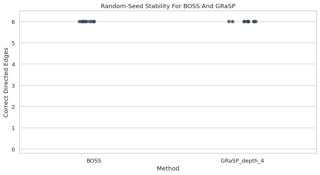
Plot Seed Stability

This plot shows recovery variation across random seeds. For a stable method and an easy dataset, the points should cluster tightly.

fig, ax = plt.subplots(figsize=(9, 5))
sns.stripplot(
    data=seed_stability_metrics,
    x="method",
    y="correct_directed_edges",
    color="#334155",
    size=7,
    alpha=0.75,
    ax=ax,
)
ax.set_title("Random-Seed Stability For BOSS And GRaSP")
ax.set_xlabel("Method")
ax.set_ylabel("Correct Directed Edges")
ax.set_ylim(-0.2, len(true_edges) + 0.5)
plt.tight_layout()
fig.savefig(FIGURE_DIR / f"{NOTEBOOK_PREFIX}_seed_stability.png", dpi=160, bbox_inches="tight")
plt.show()

Seed sensitivity serves a different role than automatically bad. It changes how results should be communicated. Stable relationships across many starts are more credible than relationships that appear in one lucky order.

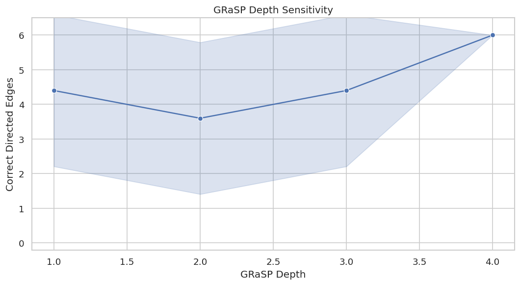
GRaSP Depth Sensitivity

GRaSP has a depth parameter controlling how deeply it searches relaxation moves. Larger depth can help escape shallow local structures, but it can also increase runtime. The code below compares several depths across a few seeds.

depth_rows = []
for depth in [1, 2, 3, 4]:
    for seed in range(5):
        _, edge_table, elapsed = run_grasp(
            linear_df,
            label=f"GRaSP_depth_{depth}_seed_{seed}",
            seed=seed,
            depth=depth,
            lambda_value=LAMBDA_VALUE,
        )
        metrics = summarize_against_truth(edge_table, true_edges, label=f"GRaSP_depth_{depth}_seed_{seed}")
        metrics["depth"] = depth
        metrics["seed"] = seed
        metrics["elapsed_seconds"] = elapsed
        depth_rows.append(metrics)
grasp_depth_metrics = pd.concat(depth_rows, ignore_index=True)
grasp_depth_summary = grasp_depth_metrics.groupby("depth", as_index=False).agg(
    runs=("seed", "count"),
    mean_correct_directed_edges=("correct_directed_edges", "mean"),
    min_correct_directed_edges=("correct_directed_edges", "min"),
    mean_extra_adjacencies=("extra_adjacencies", "mean"),
    median_elapsed_seconds=("elapsed_seconds", "median"),
)
grasp_depth_metrics.to_csv(TABLE_DIR / f"{NOTEBOOK_PREFIX}_grasp_depth_metrics.csv", index=False)
grasp_depth_summary.to_csv(TABLE_DIR / f"{NOTEBOOK_PREFIX}_grasp_depth_summary.csv", index=False)
display(grasp_depth_summary.round(4))
display(grasp_depth_metrics[["depth", "seed", "correct_directed_edges", "unresolved_true_adjacencies", "extra_adjacencies", "elapsed_seconds"]].round(4))

	depth	runs	mean_correct_directed_edges	min_correct_directed_edges	mean_extra_adjacencies	median_elapsed_seconds
0	1	5	4.4	2	0.4	0.0083
1	2	5	3.6	2	0.6	0.0079
2	3	5	4.4	2	0.4	0.0082
3	4	5	6.0	6	0.0	0.0080

	depth	seed	correct_directed_edges	unresolved_true_adjacencies	extra_adjacencies	elapsed_seconds
0	1	0	2	4	1	0.0109
1	1	1	6	0	0	0.0075
2	1	2	6	0	0	0.0090
3	1	3	6	0	0	0.0076
4	1	4	2	4	1	0.0083
5	2	0	2	4	1	0.0089
6	2	1	2	4	1	0.0067
7	2	2	6	0	0	0.0079
8	2	3	6	0	0	0.0061
9	2	4	2	4	1	0.0081
10	3	0	6	0	0	0.0088
11	3	1	2	4	1	0.0076
12	3	2	6	0	0	0.0083
13	3	3	6	0	0	0.0063
14	3	4	2	4	1	0.0082
15	4	0	6	0	0	0.0090
16	4	1	6	0	0	0.0075
17	4	2	6	0	0	0.0080
18	4	3	6	0	0	0.0056
19	4	4	6	0	0	0.0092

Depth sensitivity shows that a search setting can change the result even when the score and data are fixed. That is exactly why algorithm settings belong in the report.

Plot GRaSP Depth Sensitivity

This plot summarizes how correct directed recovery changes with depth across seeds.

fig, ax = plt.subplots(figsize=(9, 5))
sns.lineplot(
    data=grasp_depth_metrics,
    x="depth",
    y="correct_directed_edges",
    marker="o",
    errorbar="sd",
    ax=ax,
)
ax.set_title("GRaSP Depth Sensitivity")
ax.set_xlabel("GRaSP Depth")
ax.set_ylabel("Correct Directed Edges")
ax.set_ylim(-0.2, len(true_edges) + 0.5)
plt.tight_layout()
fig.savefig(FIGURE_DIR / f"{NOTEBOOK_PREFIX}_grasp_depth_sensitivity.png", dpi=160, bbox_inches="tight")
plt.show()

For this dataset, deeper search should generally be more stable. On larger datasets, depth can trade off accuracy and runtime, so it is worth tuning deliberately rather than leaving it unexplained.

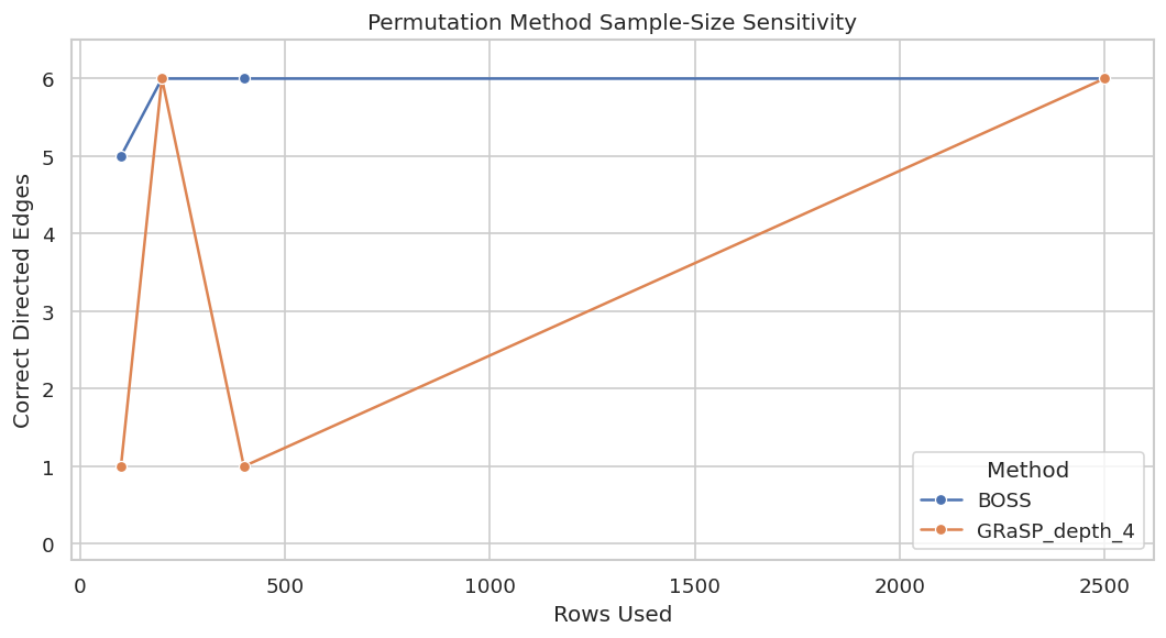
Sample-Size Sensitivity

Order-based methods still rely on local scores estimated from data. With fewer rows, local scores are noisier, and the preferred order or parent sets can change. The code below runs BOSS and GRaSP on increasing sample sizes.

sample_rows = []
for sample_size in [100, 200, 400, len(linear_df)]:
    sample_df = linear_df.sample(n=sample_size, replace=False, random_state=sample_size).reset_index(drop=True)
    for method_name in ["BOSS", "GRaSP_depth_4"]:
        if method_name == "BOSS":
            _, edge_table, elapsed = run_boss(sample_df, label=f"BOSS_n_{sample_size}", seed=BASELINE_SEED, lambda_value=LAMBDA_VALUE)
        else:
            _, edge_table, elapsed = run_grasp(sample_df, label=f"GRaSP_n_{sample_size}", seed=BASELINE_SEED, depth=GRASP_DEPTH, lambda_value=LAMBDA_VALUE)
        metrics = summarize_against_truth(edge_table, true_edges, label=f"{method_name}_n_{sample_size}")
        metrics["method"] = method_name
        metrics["sample_size"] = sample_size
        metrics["elapsed_seconds"] = elapsed
        sample_rows.append(metrics)
sample_size_metrics = pd.concat(sample_rows, ignore_index=True)
sample_size_metrics.to_csv(TABLE_DIR / f"{NOTEBOOK_PREFIX}_sample_size_metrics.csv", index=False)
display(sample_size_metrics.round(4))

	run	learned_edges_total	definite_directed_edges	true_edges	correct_directed_edges	directed_precision	directed_recall	reversed_true_edges	unresolved_true_adjacencies	missing_true_adjacencies	extra_adjacencies	method	sample_size	elapsed_seconds
0	BOSS_n_100	8	6	6	5	0.8333	0.8333	1	0	0	2	BOSS	100	0.0116
1	GRaSP_depth_4_n_100	9	6	6	1	0.1667	0.1667	2	3	0	3	GRaSP_depth_4	100	0.0057
2	BOSS_n_200	6	6	6	6	1.0000	1.0000	0	0	0	0	BOSS	200	0.0086
3	GRaSP_depth_4_n_200	6	6	6	6	1.0000	1.0000	0	0	0	0	GRaSP_depth_4	200	0.0083
4	BOSS_n_400	6	6	6	6	1.0000	1.0000	0	0	0	0	BOSS	400	0.0093
5	GRaSP_depth_4_n_400	7	4	6	1	0.2500	0.1667	2	3	0	1	GRaSP_depth_4	400	0.0108
6	BOSS_n_2500	6	6	6	6	1.0000	1.0000	0	0	0	0	BOSS	2500	0.0091
7	GRaSP_depth_4_n_2500	6	6	6	6	1.0000	1.0000	0	0	0	0	GRaSP_depth_4	2500	0.0072

Sample-size sensitivity is about evidence quality, more than runtime. A graph that appears only at one sample size deserves more caution than a graph that stabilizes as the sample grows.

Plot Sample-Size Sensitivity

This plot tracks correct directed recovery as the number of rows increases.

fig, ax = plt.subplots(figsize=(9, 5))
sns.lineplot(data=sample_size_metrics, x="sample_size", y="correct_directed_edges", hue="method", marker="o", ax=ax)
ax.set_title("Permutation Method Sample-Size Sensitivity")
ax.set_xlabel("Rows Used")
ax.set_ylabel("Correct Directed Edges")
ax.set_ylim(-0.2, len(true_edges) + 0.5)
ax.legend(title="Method")
plt.tight_layout()
fig.savefig(FIGURE_DIR / f"{NOTEBOOK_PREFIX}_sample_size_sensitivity.png", dpi=160, bbox_inches="tight")
plt.show()

The plot should be read as a stability diagnostic. It shows whether the method becomes more reliable as score estimates get more data.

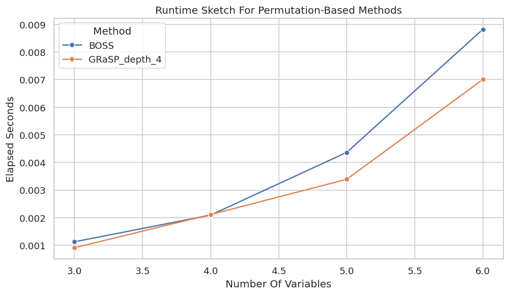
Runtime and Scaling Sketch

Permutation methods scale with variables, possible parent choices, and score evaluations. This quick sketch runs prefixes of the variable list to show how runtime changes with variable count on the same dataset.

scaling_rows = []
for variable_count in [3, 4, 5, 6]:
    cols = VARIABLES[:variable_count]
    subset_df = linear_df[cols].copy()
    for method_name in ["BOSS", "GRaSP_depth_4"]:
        if method_name == "BOSS":
            _, edge_table, elapsed = run_boss(subset_df, label=f"BOSS_p_{variable_count}", seed=BASELINE_SEED, lambda_value=LAMBDA_VALUE)
        else:
            _, edge_table, elapsed = run_grasp(subset_df, label=f"GRaSP_p_{variable_count}", seed=BASELINE_SEED, depth=GRASP_DEPTH, lambda_value=LAMBDA_VALUE)
        scaling_rows.append(
            {
                "method": method_name,
                "variable_count": variable_count,
                "elapsed_seconds": elapsed,
                "learned_edges": len(edge_table),
            }
        )
scaling_table = pd.DataFrame(scaling_rows)
scaling_table.to_csv(TABLE_DIR / f"{NOTEBOOK_PREFIX}_runtime_scaling_sketch.csv", index=False)
display(scaling_table.round(5))

	method	variable_count	elapsed_seconds	learned_edges
0	BOSS	3	0.00118	2
1	GRaSP_depth_4	3	0.00094	2
2	BOSS	4	0.00207	3
3	GRaSP_depth_4	4	0.00214	3
4	BOSS	5	0.00477	5
5	GRaSP_depth_4	5	0.00388	5
6	BOSS	6	0.00928	6
7	GRaSP_depth_4	6	0.00762	6

The absolute times are tiny here because the graph is tiny. The purpose is to show the workflow for tracking runtime as variable count grows, not to claim that all real permutation searches will be this fast.

Plot Runtime Scaling Sketch

This plot shows elapsed time by variable count for the tiny prefix runs.

fig, ax = plt.subplots(figsize=(8.5, 5))
sns.lineplot(data=scaling_table, x="variable_count", y="elapsed_seconds", hue="method", marker="o", ax=ax)
ax.set_title("Runtime Sketch For Permutation-Based Methods")
ax.set_xlabel("Number Of Variables")
ax.set_ylabel("Elapsed Seconds")
ax.legend(title="Method")
plt.tight_layout()
fig.savefig(FIGURE_DIR / f"{NOTEBOOK_PREFIX}_runtime_scaling_sketch.png", dpi=160, bbox_inches="tight")
plt.show()

For larger datasets, runtime should be measured and reported directly. Search depth, score type, parent-set complexity, and number of restarts can all change compute cost.

Reporting and Takeaways

Reporting Checklist

Permutation-based results should be reported as score-based search outputs with order-search settings. This checklist records the details that make BOSS and GRaSP analyses easier to audit.

item	what_to_report	why_it_matters
State the score function	BIC, BDeu, CV score, or another local score plus penalty settings.	The selected order and graph optimize this score, not a score-free causal criterion.
Report random seeds or restarts	Seeds used, number of starts, and whether graphs changed across starts.	Permutation search can depend on random traversal or initial order.
Document GRaSP depth	Depth setting and sensitivity results when GRaSP is used.	Depth changes the relaxation search and can change recovery.
Compare with another method	GES, PC, exact search on a small subproblem, or domain-constrained alternatives.	Agreement across search families is more reassuring than one graph alone.
Track runtime and graph size	Elapsed time, variable count, learned edge count, and any parent limits.	Order search can become expensive as graph size and score complexity grow.
Separate optimization from causality	What was optimized and which causal assumptions are still required.	A high-scoring permutation is not causal proof by itself.

The checklist is deliberately practical. It keeps the final graph connected to the score, search settings, stability checks, and assumptions that produced it.

For causal discovery, the result is a statement about recoverable structure under assumptions, not a free-standing proof of cause and effect.

Summary

This section now gives a complete permutation-based discovery workflow covering order-search theory, fixed-order parent selection, BOSS and GRaSP runs, comparison with GES and exact search, seed stability, GRaSP depth sensitivity, sample-size sensitivity, runtime sketching, and reporting guidance.

The sequence next moves to time-series causal discovery, where lag structure provides another source of direction information.

Previous Tutorial11: Functional Causal Models: ANM and PNL Tutorial Homecausal-learn tutorial series Next Tutorial13: Time-Series Causal Discovery