causal-learn Tutorial 09: Exact Search And Score Functions

The previous notebook introduced GES, a greedy score-based search method. GES is fast and practical, but it is still greedy: it follows local score improvements rather than proving that no better graph exists anywhere in the search space.

This notebook studies exact score-based search. Exact search asks a sharper question: among all DAGs allowed by a search space, which graph optimizes the score? In causal-learn, bic_exact_search solves this problem for a BIC-style continuous score using dynamic programming or A* search over an order graph.

Exact search is valuable for teaching and benchmarking because it shows what the best-scoring graph is under a score. But it is not a magic replacement for scalable discovery. The number of possible parent sets and variable orderings grows explosively with the number of variables, so exact search is usually reserved for small graphs, constrained graphs, or benchmarking smaller subproblems.

Runtime Note

This notebook is designed to run quickly by default, usually under 1-2 minutes in this workspace. The exact-search examples use six or fewer variables and small structural constraints.

Exact search can become long-running when the number of variables grows. The notebook includes scaling diagnostics to show why. If you later try exact search on 10, 15, or more variables without strong constraints, runtime and memory can grow very quickly.

Notebook Flow

We will work through exact score-based discovery in this order:

1. Set up imports, paths, exact search, GES, and graph helpers.
2. Load the linear Gaussian teaching dataset and known synthetic graph.
3. Explain exact search, BIC local scores, A* search, dynamic programming, and super-structures.
4. Run exact BIC search with A* and DP and compare their search statistics.
5. Inspect local parent-set scores for one node.
6. Compare the exact graph with GES on the same data.
7. Use super-structures and max-parent constraints to show how prior search-space restrictions affect exact search.
8. Study sample-size and variable-count scaling.
9. Save a reporting checklist and artifact manifest.

Every code cell has explanatory text before it and a short discussion after it, matching the style of the earlier tutorial notebooks.

Exact Search Theory

Exact score-based search asks a precise optimization question: among all DAGs in the allowed search space, which graph has the best score?

This is different from GES. GES is greedy and follows local score improvements. Exact search uses dynamic programming or A* search to guarantee the optimum for the chosen score and constraints, at least within the graph size the algorithm can handle.

The phrase “exact” is easy to overread. Exact search is exact for the mathematical optimization problem it solves. It is not exact causal truth independent of score assumptions, sample noise, hidden variables, or model mismatch.

DAG Search Space Grows Explosively

The number of possible DAGs grows super-exponentially with the number of variables. Even modest increases in variable count can make exhaustive search infeasible.

This is why exact search is usually used for small graphs, constrained subproblems, benchmarking, or teaching. It gives a valuable reference point: if GES and exact search agree on a small problem, we gain confidence that the greedy method found the global optimum for that score.

If they disagree, exact search helps reveal where greedy search got stuck or where constraints changed the optimal graph.

Local Scores And Parent Sets

Most exact DAG search methods rely on decomposable scores:

\[ S(G) = \sum_i S_i(\mathrm{Pa}(X_i)) \]

This means each node’s contribution depends only on its parent set. Exact search can precompute or cache scores for candidate parent sets, then combine those local choices while enforcing acyclicity.

The parent-set view is central. Instead of thinking “try every graph,” it is better to think “score possible parent sets for each node, then search for a compatible acyclic combination.”

Parent Graphs And Order Graphs

A parent graph stores candidate parent sets and their local scores for each target variable. If a node has many possible parents, the number of candidate parent sets grows quickly.

An order graph represents possible variable orderings. A DAG is acyclic if its edges are consistent with at least one topological order. Searching over orders can therefore help enforce acyclicity without enumerating every DAG directly.

Dynamic programming and A* search use these structures to avoid redundant work. They are still expensive, but much smarter than naive enumeration.

Dynamic Programming Versus A* Search

Dynamic programming solves the exact search problem by building optimal solutions for smaller subsets of variables and combining them into larger solutions. It is systematic and exact, but memory can grow quickly because many subsets must be considered.

A* search treats the problem as a shortest-path or best-first search through an order graph. It uses a heuristic to prioritize promising partial orders and can be faster when the heuristic is informative.

Both methods are exact only when their assumptions and search settings preserve the full allowed search space. Constraints such as maximum parent count, super-graphs, or required edges change the optimization problem.

Constraints: Super-Graphs, Required Edges, And Max Parents

Exact search becomes more practical when the search space is constrained.

A super-graph says which edges are allowed. Exact search then finds the best DAG inside that allowed edge set. If the super-graph excludes a true edge, the exact optimum cannot recover it.

A required-edge constraint forces certain relationships to appear. This can encode strong domain knowledge but can also force a wrong graph.

A max-parent constraint limits how many parents each node may have. This reduces computation and can reduce overfitting, but it can also exclude real multi-parent mechanisms.

What Exact Search Can And Cannot Claim

Exact search can certify that no other allowed DAG scores better under the chosen score. That is powerful for benchmarking and for small, well-constrained problems.

It cannot rescue a bad score, bad data, hidden confounding, or an excluded true graph. It can also be unstable across sample sizes because the best-scoring graph for a small noisy sample may differ from the best-scoring graph for the population.

A good exact-search report states the score, constraints, variable count, parent limits, runtime, memory concerns, and whether “exact” means exact over all DAGs or exact only over a restricted search space.

Setup

The setup cell imports causal-learn’s exact BIC search, GES for comparison, plotting tools, and utilities for clean output. It also applies the same local BIC compatibility wrapper used in the GES notebook so GES comparison runs work under the current NumPy behavior. ExactSearch’s own BIC scoring path does not need that wrapper.

from pathlib import Path
from importlib.metadata import PackageNotFoundError, version
import contextlib
import io
import itertools
import os
import time
import warnings

# Keep matplotlib cache writes inside the repository so notebook execution works in restricted environments.
os.environ.setdefault("MPLCONFIGDIR", str(Path.cwd() / ".matplotlib_cache"))
warnings.filterwarnings("ignore", message="IProgress not found.*")
warnings.filterwarnings("ignore", message=".*pkg_resources is deprecated.*")

import numpy as np
import pandas as pd
import matplotlib.pyplot as plt
import seaborn as sns
from IPython.display import display
from matplotlib.patches import FancyArrowPatch, FancyBboxPatch

from causallearn.search.ScoreBased.ExactSearch import bic_exact_search, bic_score_node, generate_parent_graph
import causallearn.search.ScoreBased.GES as ges_module
from causallearn.search.ScoreBased.GES import ges

# Resolve paths whether the notebook is run from the repository root or from this notebook folder.
CWD = Path.cwd()
if CWD.name == "causal_learn" and (CWD / "outputs").exists():
    NOTEBOOK_DIR = CWD
else:
    NOTEBOOK_DIR = (CWD / "notebooks" / "tutorials" / "causal_learn").resolve()

OUTPUT_DIR = NOTEBOOK_DIR / "outputs"
DATASET_DIR = OUTPUT_DIR / "datasets"
TABLE_DIR = OUTPUT_DIR / "tables"
FIGURE_DIR = OUTPUT_DIR / "figures"
for directory in [OUTPUT_DIR, DATASET_DIR, TABLE_DIR, FIGURE_DIR]:
    directory.mkdir(parents=True, exist_ok=True)

NOTEBOOK_PREFIX = "09"
sns.set_theme(style="whitegrid", context="notebook")
plt.rcParams["figure.dpi"] = 120
plt.rcParams["savefig.facecolor"] = "white"


def local_score_BIC_from_cov(Data, i, PAi, parameters=None):
    """Compatibility wrapper for causal-learn GES BIC scoring under recent NumPy scalar behavior."""
    cov, n = Data
    lambda_value = 0.5 if parameters is None else parameters.get("lambda_value", 0.5)
    sigma = float(cov[i, i])
    if len(PAi) > 0:
        yX = cov[np.ix_([i], PAi)]
        XX = cov[np.ix_(PAi, PAi)]
        try:
            XX_inv = np.linalg.inv(XX)
        except np.linalg.LinAlgError:
            XX_inv = np.linalg.pinv(XX)
        sigma = float(cov[i, i] - (yX @ XX_inv @ yX.T).item())
    sigma = max(sigma, 1e-12)
    return -0.5 * n * (1 + np.log(sigma)) - lambda_value * (len(PAi) + 1) * np.log(n)

# Patch only the imported module object used by GES during this notebook session.
ges_module.local_score_BIC_from_cov = local_score_BIC_from_cov

packages = ["causal-learn", "numpy", "pandas", "matplotlib", "seaborn"]
version_rows = []
for package in packages:
    try:
        package_version = version(package)
    except PackageNotFoundError:
        package_version = "not installed"
    version_rows.append({"package": package, "version": package_version})

package_versions = pd.DataFrame(version_rows)
package_versions.to_csv(TABLE_DIR / f"{NOTEBOOK_PREFIX}_package_versions.csv", index=False)
display(package_versions)

	package	version
0	causal-learn	0.1.4.5
1	numpy	2.4.4
2	pandas	3.0.2
3	matplotlib	3.10.9
4	seaborn	0.13.2

The version table and local GES wrapper make the comparison reproducible. The exact-search examples themselves rely on causal-learn’s bic_exact_search and bic_score_node functions.

Load The Linear Gaussian Teaching Data

Exact BIC search uses a continuous BIC score, so we use the linear Gaussian dataset from the synthetic data notebook. This is the same friendly setting where BIC-GES performed well.

# Load the linear Gaussian data and the known synthetic true edge list.
linear_path = DATASET_DIR / "02_linear_gaussian.csv"
true_edge_path = TABLE_DIR / "02_base_true_dag_edges.csv"

required_paths = [linear_path, true_edge_path]
missing_paths = [str(path) for path in required_paths if not path.exists()]
if missing_paths:
    raise FileNotFoundError("Run tutorial notebook 02 first. Missing files: " + ", ".join(missing_paths))

linear_df = pd.read_csv(linear_path)
true_edges = pd.read_csv(true_edge_path)
VARIABLES = list(linear_df.columns)

loaded_summary = pd.DataFrame(
    [
        {
            "dataset": "linear_gaussian",
            "rows": len(linear_df),
            "columns": linear_df.shape[1],
            "missing_cells": int(linear_df.isna().sum().sum()),
            "source_file": linear_path.name,
        }
    ]
)
loaded_summary.to_csv(TABLE_DIR / f"{NOTEBOOK_PREFIX}_loaded_dataset_summary.csv", index=False)

display(loaded_summary)
display(linear_df.head())
display(true_edges)

	dataset	rows	columns	missing_cells	source_file
0	linear_gaussian	2500	6	0	02_linear_gaussian.csv

	need	intent	match	engagement	renewal	support
0	0.249820	-0.372094	0.060245	0.667197	0.252766	-0.280058
1	0.683671	-0.210471	0.904969	1.004727	0.320095	-0.332215
2	-0.579752	-1.202671	-0.578579	-0.235444	-0.732431	0.594102
3	-0.902823	-0.077309	-0.771219	-0.531128	-0.105721	-1.503551
4	-1.985745	0.087297	-0.691315	-1.281731	-0.797906	-0.328219

	source	target	edge_type	mechanism
0	need	match	directed	Need changes what a good match means.
1	intent	match	directed	Current intent changes recommendation relevance.
2	match	engagement	directed	Better matching increases engagement depth.
3	intent	renewal	directed	Intent directly affects later value.
4	engagement	renewal	directed	Engagement contributes to renewal value.
5	engagement	support	directed	Engagement creates more chances for support co...

The data are small enough in variable count for exact search and large enough in rows for stable local score estimates. The true graph will be used only for tutorial evaluation.

Exact Search Concept Map

Before running code, we define the key pieces. Exact search is not simply “try every DAG one by one.” causal-learn uses dynamic programming or A* over an order graph, with local parent-set scores cached for each node.

# Summarize exact-search concepts used in this notebook.
concept_map = pd.DataFrame(
    [
        {
            "concept": "local BIC score",
            "plain_language": "Score one node given a proposed parent set.",
            "why_it_matters": "Decomposable scores let the total graph score be built from local node scores.",
        },
        {
            "concept": "parent graph",
            "plain_language": "For each node, cache the best parent set available under different candidate predecessors.",
            "why_it_matters": "Parent-set caching makes exact search much faster than naive enumeration.",
        },
        {
            "concept": "order graph",
            "plain_language": "Search over subsets or variable orderings rather than every DAG directly.",
            "why_it_matters": "Dynamic programming and A* use this structure to find an optimal DAG for the score.",
        },
        {
            "concept": "A* exact search",
            "plain_language": "Use a priority queue and heuristic to search promising order-graph states first.",
            "why_it_matters": "Can visit fewer states than full dynamic programming on some problems.",
        },
        {
            "concept": "super-structure",
            "plain_language": "Restrict which edges are allowed before search begins.",
            "why_it_matters": "Good constraints reduce runtime; invalid constraints can force a wrong graph.",
        },
    ]
)
concept_map.to_csv(TABLE_DIR / f"{NOTEBOOK_PREFIX}_exact_search_concept_map.csv", index=False)
display(concept_map)

	concept	plain_language	why_it_matters
0	local BIC score	Score one node given a proposed parent set.	Decomposable scores let the total graph score ...
1	parent graph	For each node, cache the best parent set avail...	Parent-set caching makes exact search much fas...
2	order graph	Search over subsets or variable orderings rath...	Dynamic programming and A* use this structure ...
3	A* exact search	Use a priority queue and heuristic to search p...	Can visit fewer states than full dynamic progr...
4	super-structure	Restrict which edges are allowed before search...	Good constraints reduce runtime; invalid const...

The concept map frames exact search as optimized exhaustive search over a constrained space. The exact result is exact for the score and constraints, not exact causal truth in a universal sense.

Helper Functions

This helper cell converts adjacency matrices into edge tables, computes scores and graph metrics, and draws rounded-box graphs using the same visual style as earlier notebooks.

def adjacency_to_edge_table(adjacency, variables, label):
    """Convert a parent-row, child-column adjacency matrix into a tidy directed edge table."""
    rows = []
    for parent_idx, child_idx in zip(*np.where(adjacency > 0)):
        rows.append(
            {
                "run": label,
                "source": variables[int(parent_idx)],
                "edge_type": "-->",
                "target": variables[int(child_idx)],
            }
        )
    return pd.DataFrame(rows, columns=["run", "source", "edge_type", "target"])


def parse_causallearn_edge(edge):
    """Convert a causal-learn edge object into source, endpoint pattern, and target strings."""
    parts = str(edge).strip().split()
    if len(parts) != 3:
        return {"source": str(edge), "edge_type": "unknown", "target": "unknown"}
    return {"source": parts[0], "edge_type": parts[1], "target": parts[2]}


def graph_to_edge_table(graph, label):
    """Return a tidy edge table from a causal-learn graph object."""
    rows = [parse_causallearn_edge(edge) for edge in graph.get_graph_edges()]
    edge_df = pd.DataFrame(rows, columns=["source", "edge_type", "target"])
    if edge_df.empty:
        edge_df = pd.DataFrame(columns=["source", "edge_type", "target"])
    edge_df.insert(0, "run", label)
    return edge_df


def directed_pairs(edge_df):
    """Extract definite directed pairs from an edge table."""
    pairs = set()
    for row in edge_df.itertuples(index=False):
        if row.edge_type == "-->":
            pairs.add((row.source, row.target))
        elif row.edge_type == "<--":
            pairs.add((row.target, row.source))
    return pairs


def skeleton_pairs(edge_df):
    """Extract adjacencies while ignoring direction."""
    pairs = set()
    for row in edge_df.itertuples(index=False):
        if row.target != "unknown":
            pairs.add(frozenset([row.source, row.target]))
    return pairs


def summarize_against_truth(edge_df, truth_df, label):
    """Compute compact graph-recovery metrics against a truth table."""
    true_directed = set(zip(truth_df["source"], truth_df["target"]))
    true_skeleton = {frozenset(edge) for edge in true_directed}
    learned_directed = directed_pairs(edge_df)
    learned_skeleton = skeleton_pairs(edge_df)

    correct_directed = learned_directed & true_directed
    reversed_true = {(src, dst) for src, dst in true_directed if (dst, src) in learned_directed}
    missing_skeleton = true_skeleton - learned_skeleton
    extra_skeleton = learned_skeleton - true_skeleton

    unresolved_true = 0
    for src, dst in true_directed:
        pair = frozenset([src, dst])
        if pair in learned_skeleton and (src, dst) not in learned_directed and (dst, src) not in learned_directed:
            unresolved_true += 1

    directed_count = len(learned_directed)
    return pd.DataFrame(
        [
            {
                "run": label,
                "learned_edges_total": len(edge_df),
                "definite_directed_edges": directed_count,
                "true_edges": len(true_directed),
                "correct_directed_edges": len(correct_directed),
                "directed_precision": len(correct_directed) / directed_count if directed_count else np.nan,
                "directed_recall": len(correct_directed) / len(true_directed) if true_directed else np.nan,
                "reversed_true_edges": len(reversed_true),
                "unresolved_true_adjacencies": unresolved_true,
                "missing_true_adjacencies": len(missing_skeleton),
                "extra_adjacencies": len(extra_skeleton),
            }
        ]
    )


def total_exact_bic_score(data, adjacency):
    """Compute the total ExactSearch BIC score for a given adjacency matrix. Lower is better."""
    total = 0.0
    for child_idx in range(adjacency.shape[1]):
        parents = tuple(np.where(adjacency[:, child_idx] > 0)[0])
        total += float(bic_score_node(data, child_idx, parents))
    return total


def edge_table_to_adjacency(edge_df, variables):
    """Convert a directed edge table to an adjacency matrix using source rows and target columns."""
    index = {name: i for i, name in enumerate(variables)}
    adjacency = np.zeros((len(variables), len(variables)))
    for row in edge_df.itertuples(index=False):
        if row.edge_type == "-->" and row.source in index and row.target in index:
            adjacency[index[row.source], index[row.target]] = 1
        elif row.edge_type == "<--" and row.source in index and row.target in index:
            adjacency[index[row.target], index[row.source]] = 1
    return adjacency


def run_exact_search(data_df, label, search_method="astar", super_graph=None, include_graph=None, max_parents=None):
    """Run exact BIC search and return adjacency, edge table, stats, and elapsed time."""
    start = time.perf_counter()
    adjacency, stats = bic_exact_search(
        data_df.to_numpy(),
        super_graph=super_graph,
        search_method=search_method,
        use_path_extension=True,
        verbose=False,
        include_graph=include_graph,
        max_parents=max_parents,
    )
    elapsed = time.perf_counter() - start
    edge_table = adjacency_to_edge_table(adjacency, list(data_df.columns), label=label)
    return adjacency, edge_table, stats, elapsed


def run_ges_bic(data_df, label):
    """Run BIC-GES quietly for comparison."""
    buffer = io.StringIO()
    with contextlib.redirect_stdout(buffer):
        record = ges(
            data_df.to_numpy(),
            score_func="local_score_BIC",
            node_names=list(data_df.columns),
            lambda_value=0.5,
        )
    edge_table = graph_to_edge_table(record["G"], label=label)
    return record, edge_table


GRAPH_POSITIONS = {
    "need": (0.11, 0.72),
    "intent": (0.11, 0.28),
    "match": (0.39, 0.50),
    "engagement": (0.62, 0.50),
    "renewal": (0.89, 0.72),
    "support": (0.89, 0.28),
}
NODE_LABELS = {name: name.title() for name in GRAPH_POSITIONS}
NODE_COLORS = {
    "need": "#e0f2fe",
    "intent": "#dbeafe",
    "match": "#ecfccb",
    "engagement": "#fef3c7",
    "renewal": "#fee2e2",
    "support": "#f3e8ff",
}


def trim_edge_to_box(start, end, box_w=0.145, box_h=0.095, gap=0.012):
    """Return edge endpoints that stop just outside source and target boxes."""
    x0, y0 = start
    x1, y1 = end
    dx = x1 - x0
    dy = y1 - y0
    length = float(np.hypot(dx, dy))
    if length == 0:
        return start, end
    effective_w = box_w + 0.04
    effective_h = box_h + 0.04
    x_limit = (effective_w / 2) / abs(dx) if dx else np.inf
    y_limit = (effective_h / 2) / abs(dy) if dy else np.inf
    t = min(x_limit, y_limit) + gap / length
    return (x0 + dx * t, y0 + dy * t), (x1 - dx * t, y1 - dy * t)


def draw_box_graph(edge_df, title, path, note=None):
    """Draw a DAG-style graph with rounded boxes and visible arrowheads."""
    fig, ax = plt.subplots(figsize=(12, 6.2))
    ax.set_axis_off()
    ax.set_xlim(-0.02, 1.02)
    ax.set_ylim(0.04, 0.96)
    box_w, box_h = 0.145, 0.095

    for row in edge_df.itertuples(index=False):
        if row.source not in GRAPH_POSITIONS or row.target not in GRAPH_POSITIONS:
            continue
        raw_start = GRAPH_POSITIONS[row.source]
        raw_end = GRAPH_POSITIONS[row.target]
        if row.edge_type == "<--":
            raw_start, raw_end = raw_end, raw_start
        start, end = trim_edge_to_box(raw_start, raw_end, box_w=box_w, box_h=box_h)
        if row.edge_type in {"-->", "<--"}:
            arrowstyle = "-|>"
            mutation_scale = 18
            linewidth = 1.8
            color = "#334155"
        else:
            arrowstyle = "-"
            mutation_scale = 1
            linewidth = 1.5
            color = "#64748b"
        arrow = FancyArrowPatch(
            start,
            end,
            arrowstyle=arrowstyle,
            mutation_scale=mutation_scale,
            linewidth=linewidth,
            color=color,
            connectionstyle="arc3,rad=0.035",
            zorder=2,
        )
        ax.add_patch(arrow)

    for node, (x, y) in GRAPH_POSITIONS.items():
        rect = FancyBboxPatch(
            (x - box_w / 2, y - box_h / 2),
            box_w,
            box_h,
            boxstyle="round,pad=0.018",
            facecolor=NODE_COLORS[node],
            edgecolor="#1f2937",
            linewidth=1.1,
            zorder=5,
        )
        ax.add_patch(rect)
        ax.text(x, y, NODE_LABELS[node], ha="center", va="center", fontsize=10.5, fontweight="bold", zorder=6)

    if note:
        ax.text(0.50, 0.08, note, ha="center", va="center", fontsize=10, color="#475569")
    ax.set_title(title, pad=18, fontsize=14, fontweight="bold")
    fig.savefig(path, dpi=160, bbox_inches="tight")
    plt.show()


def truth_as_edge_table(truth_df, label="truth"):
    """Convert a truth table into a plotting-ready edge table."""
    return truth_df.assign(run=label, edge_type="-->")[["run", "source", "edge_type", "target"]]

The helpers give the rest of the notebook a compact vocabulary: exact-search adjacency matrices become edge tables, edge tables become metrics, and every graph is drawn in the same style.

Draw The Reference DAG

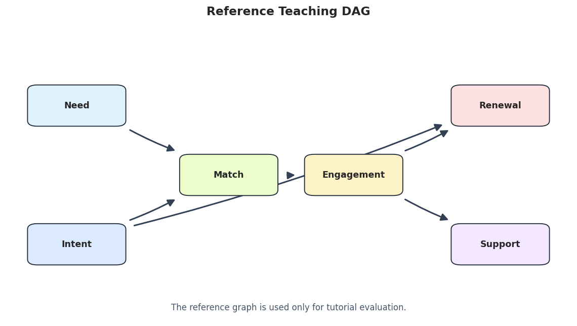
We draw the known synthetic graph first so exact search results have a visual target. In applied work this graph would not be known.

# Draw the reference synthetic graph.
true_edge_table = truth_as_edge_table(true_edges, label="true_graph")
true_graph_path = FIGURE_DIR / f"{NOTEBOOK_PREFIX}_true_dag.png"
draw_box_graph(
    true_edge_table,
    title="Reference Teaching DAG",
    path=true_graph_path,
    note="The reference graph is used only for tutorial evaluation.",
)

The reference graph has six directed edges. Exact BIC search will now look for the best-scoring DAG under its own score, not for this graph directly.

Exact BIC Search With A* And Dynamic Programming

causal-learn supports two exact-search methods here: A* and dynamic programming. Both should return the same optimal DAG under the same score and constraints. Their search statistics can differ because they traverse the order graph differently.

# Run exact BIC search with A* and dynamic programming.
exact_runs = []
exact_edge_tables = []
for method in ["astar", "dp"]:
    label = f"exact_bic_{method}"
    adjacency, edge_table, stats, elapsed = run_exact_search(
        linear_df,
        label=label,
        search_method=method,
        max_parents=None,
    )
    metrics = summarize_against_truth(edge_table, true_edges, label)
    exact_runs.append(
        {
            "run": label,
            "search_method": method,
            "elapsed_seconds": elapsed,
            "exact_bic_score_lower_is_better": total_exact_bic_score(linear_df.to_numpy(), adjacency),
            "learned_edge_count": int(adjacency.sum()),
            **stats,
        }
    )
    exact_edge_tables.append(edge_table.assign(search_method=method))

exact_search_stats = pd.DataFrame(exact_runs)
exact_search_edges = pd.concat(exact_edge_tables, ignore_index=True)
exact_search_metrics = pd.concat(
    [summarize_against_truth(table.drop(columns=["search_method"]), true_edges, table["run"].iloc[0]) for _, table in exact_search_edges.groupby("run")],
    ignore_index=True,
)

exact_search_stats.to_csv(TABLE_DIR / f"{NOTEBOOK_PREFIX}_exact_search_stats.csv", index=False)
exact_search_edges.to_csv(TABLE_DIR / f"{NOTEBOOK_PREFIX}_exact_search_edges.csv", index=False)
exact_search_metrics.to_csv(TABLE_DIR / f"{NOTEBOOK_PREFIX}_exact_search_metrics.csv", index=False)

display(exact_search_stats)
display(exact_search_edges)
display(exact_search_metrics)

	run	search_method	elapsed_seconds	exact_bic_score_lower_is_better	learned_edge_count	n_parent_graphs_entries	while_iter	for_iter	n_closed	max_n_opened	n_order_graph_nodes	n_order_graph_edges
0	exact_bic_astar	astar	0.024491	-9950.952924	6	109	36.0	120.0	36.0	20.0	NaN	NaN
1	exact_bic_dp	dp	0.015681	-9950.952924	6	109	NaN	NaN	NaN	NaN	64.0	148.0

	run	source	edge_type	target	search_method
0	exact_bic_astar	need	-->	match	astar
1	exact_bic_astar	intent	-->	match	astar
2	exact_bic_astar	intent	-->	renewal	astar
3	exact_bic_astar	match	-->	engagement	astar
4	exact_bic_astar	engagement	-->	renewal	astar
5	exact_bic_astar	engagement	-->	support	astar
6	exact_bic_dp	need	-->	match	dp
7	exact_bic_dp	intent	-->	match	dp
8	exact_bic_dp	intent	-->	renewal	dp
9	exact_bic_dp	match	-->	engagement	dp
10	exact_bic_dp	engagement	-->	renewal	dp
11	exact_bic_dp	engagement	-->	support	dp

	run	learned_edges_total	definite_directed_edges	true_edges	correct_directed_edges	directed_precision	directed_recall	reversed_true_edges	unresolved_true_adjacencies	missing_true_adjacencies	extra_adjacencies
0	exact_bic_astar	6	6	6	6	1.0	1.0	0	0	0	0
1	exact_bic_dp	6	6	6	6	1.0	1.0	0	0	0	0

A* and dynamic programming return the same graph, as expected. The statistics show the machinery behind exact search: parent-graph entries, order-graph nodes, and search iterations.

Draw The Exact BIC Graph

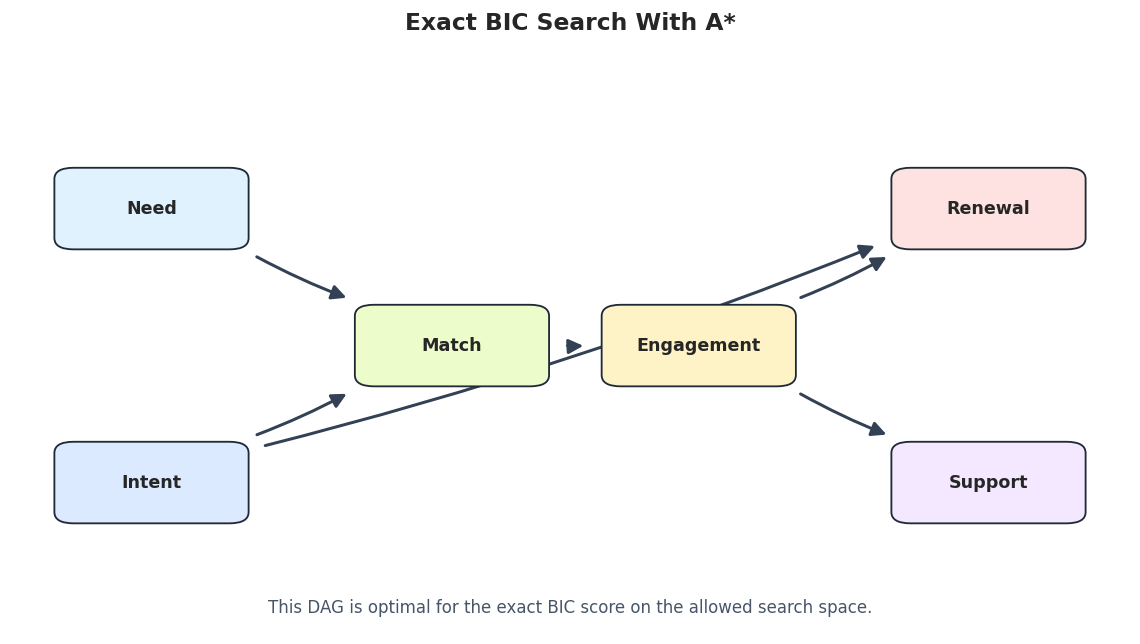
The exact graph is the best-scoring DAG under causal-learn’s exact BIC objective and the unconstrained six-variable search space.

# Draw the A* exact-search graph.
exact_astar_edges = exact_search_edges[exact_search_edges["run"] == "exact_bic_astar"].drop(columns=["search_method"])
exact_graph_path = FIGURE_DIR / f"{NOTEBOOK_PREFIX}_exact_bic_astar_graph.png"
draw_box_graph(
    exact_astar_edges,
    title="Exact BIC Search With A*",
    path=exact_graph_path,
    note="This DAG is optimal for the exact BIC score on the allowed search space.",
)

In this friendly synthetic case, the exact BIC graph matches the reference DAG. The next section opens the local score logic that makes exact search possible.

Local Parent-Set Scores For match

Exact search works because the graph score decomposes by node. Here we focus on the match node and score possible parent sets. Lower BIC values are better for bic_score_node.

# Score candidate parent sets for the match node.
match_index = VARIABLES.index("match")
candidate_parent_names = [name for name in VARIABLES if name != "match"]
parent_score_rows = []
for parent_count in range(0, 4):
    for parent_names in itertools.combinations(candidate_parent_names, parent_count):
        parent_indices = tuple(VARIABLES.index(name) for name in parent_names)
        score = bic_score_node(linear_df.to_numpy(), match_index, parent_indices)
        parent_score_rows.append(
            {
                "child": "match",
                "parent_set": list(parent_names),
                "parent_count": parent_count,
                "local_bic_score_lower_is_better": float(score),
            }
        )

match_parent_scores = pd.DataFrame(parent_score_rows).sort_values("local_bic_score_lower_is_better")
match_parent_scores.to_csv(TABLE_DIR / f"{NOTEBOOK_PREFIX}_match_parent_set_scores.csv", index=False)
display(match_parent_scores.head(15))

	child	parent_set	parent_count	local_bic_score_lower_is_better
16	match	[need, intent, engagement]	3	-4479.089770
18	match	[need, intent, support]	3	-3667.015172
17	match	[need, intent, renewal]	3	-3648.117337
19	match	[need, engagement, renewal]	3	-3556.411652
6	match	[need, intent]	2	-3516.479864
10	match	[intent, engagement]	2	-3275.416951
23	match	[intent, engagement, support]	3	-3269.316850
22	match	[intent, engagement, renewal]	3	-3268.865824
7	match	[need, engagement]	2	-3180.792129
20	match	[need, engagement, support]	3	-3173.301495
13	match	[engagement, renewal]	2	-2976.977150
25	match	[engagement, renewal, support]	3	-2971.060530
21	match	[need, renewal, support]	3	-2811.884480
3	match	[engagement]	1	-2793.639587
14	match	[engagement, support]	2	-2787.203378

The best local parent sets for match include need and intent, which are its true direct parents in the synthetic graph. This local view explains part of why the full exact search recovers the intended structure.

Parent Graph Size For Each Node

Exact search caches possible parent sets in a parent graph for each target node. This cell counts how many parent-graph entries are generated for each node with and without a max-parent limit.

# Count parent-graph entries for each node under different max-parent settings.
parent_graph_rows = []
for max_parents in [1, 2, 3, len(VARIABLES)]:
    for node_idx, node_name in enumerate(VARIABLES):
        parent_graph = generate_parent_graph(
            linear_df.to_numpy(),
            node_idx,
            max_parents=max_parents,
        )
        parent_graph_rows.append(
            {
                "node": node_name,
                "max_parents": max_parents,
                "parent_graph_entries": len(parent_graph),
                "best_parent_set": [VARIABLES[int(idx)] for idx in parent_graph[0][0]],
                "best_local_bic_score_lower_is_better": float(parent_graph[0][1]),
            }
        )

parent_graph_summary = pd.DataFrame(parent_graph_rows)
parent_graph_summary.to_csv(TABLE_DIR / f"{NOTEBOOK_PREFIX}_parent_graph_entry_summary.csv", index=False)
display(parent_graph_summary)

	node	max_parents	parent_graph_entries	best_parent_set	best_local_bic_score_lower_is_better
0	need	1	5	[match]	-1084.757041
1	intent	1	5	[renewal]	-1936.585079
2	match	1	6	[engagement]	-2793.639587
3	engagement	1	6	[match]	-2793.639587
4	renewal	1	6	[intent]	-1936.585079
5	support	1	6	[engagement]	-1026.510792
6	need	2	12	[intent, match]	-2208.258093
7	intent	2	11	[need, match]	-2424.006541
8	match	2	15	[need, intent]	-3516.479864
9	engagement	2	14	[match, support]	-3139.027763
10	renewal	2	15	[intent, engagement]	-2614.322682
11	support	2	9	[engagement]	-1026.510792
12	need	3	15	[intent, match]	-2208.258093
13	intent	3	16	[need, match, renewal]	-3031.723569
14	match	3	21	[need, intent, engagement]	-4479.089770
15	engagement	3	21	[match, renewal, support]	-3333.751321
16	renewal	3	19	[intent, engagement]	-2614.322682
17	support	3	12	[engagement]	-1026.510792
18	need	6	15	[intent, match]	-2208.258093
19	intent	6	17	[need, match, engagement, renewal]	-3078.467264
20	match	6	22	[need, intent, engagement]	-4479.089770
21	engagement	6	24	[intent, match, renewal, support]	-3399.985399
22	renewal	6	19	[intent, engagement]	-2614.322682
23	support	6	12	[engagement]	-1026.510792

The parent-graph table shows why max-parent limits can matter. Smaller limits reduce the number of local structures considered, but they are only safe if the true graph does not require larger parent sets.

Compare Exact Search With GES

GES is greedy, while exact search optimizes the BIC objective over the allowed DAG space. On this friendly dataset, both methods should agree. That agreement is useful because it tells us the greedy method did not get trapped in a worse local solution here.

# Run GES for comparison with exact BIC search.
ges_record, ges_edges = run_ges_bic(linear_df, label="bic_ges_linear_gaussian")
ges_adjacency = edge_table_to_adjacency(ges_edges, VARIABLES)
ges_metrics = summarize_against_truth(ges_edges, true_edges, "bic_ges_linear_gaussian")
exact_metrics = summarize_against_truth(exact_astar_edges, true_edges, "exact_bic_astar")

exact_vs_ges = pd.concat([exact_metrics, ges_metrics], ignore_index=True)
score_comparison = pd.DataFrame(
    [
        {
            "run": "exact_bic_astar",
            "exact_bic_score_lower_is_better": total_exact_bic_score(linear_df.to_numpy(), edge_table_to_adjacency(exact_astar_edges, VARIABLES)),
            "learned_edges_total": len(exact_astar_edges),
        },
        {
            "run": "bic_ges_linear_gaussian",
            "exact_bic_score_lower_is_better": total_exact_bic_score(linear_df.to_numpy(), ges_adjacency),
            "learned_edges_total": len(ges_edges),
        },
    ]
)

exact_vs_ges.to_csv(TABLE_DIR / f"{NOTEBOOK_PREFIX}_exact_vs_ges_metrics.csv", index=False)
score_comparison.to_csv(TABLE_DIR / f"{NOTEBOOK_PREFIX}_exact_vs_ges_score_comparison.csv", index=False)
ges_edges.to_csv(TABLE_DIR / f"{NOTEBOOK_PREFIX}_ges_comparison_edges.csv", index=False)

display(score_comparison)
display(exact_vs_ges)
display(ges_edges)

	run	exact_bic_score_lower_is_better	learned_edges_total
0	exact_bic_astar	-9950.952924	6
1	bic_ges_linear_gaussian	-9950.952924	6

	run	learned_edges_total	definite_directed_edges	true_edges	correct_directed_edges	directed_precision	directed_recall	reversed_true_edges	unresolved_true_adjacencies	missing_true_adjacencies	extra_adjacencies
0	exact_bic_astar	6	6	6	6	1.0	1.0	0	0	0	0
1	bic_ges_linear_gaussian	6	6	6	6	1.0	1.0	0	0	0	0

	run	source	edge_type	target
0	bic_ges_linear_gaussian	need	-->	match
1	bic_ges_linear_gaussian	intent	-->	match
2	bic_ges_linear_gaussian	intent	-->	renewal
3	bic_ges_linear_gaussian	match	-->	engagement
4	bic_ges_linear_gaussian	engagement	-->	renewal
5	bic_ges_linear_gaussian	engagement	-->	support

Exact search and GES agree in this case. That is reassuring, but it should not be assumed in every dataset. Exact search is most useful as a benchmark for small problems where the global optimum can actually be computed.

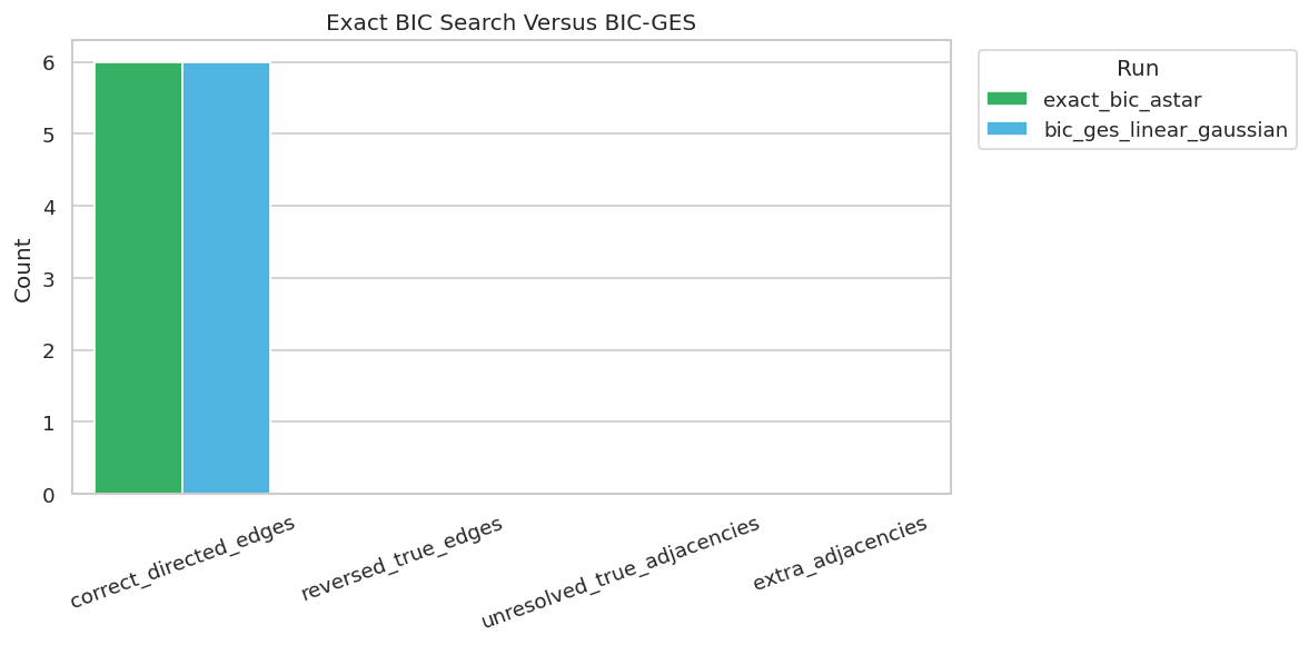
Plot Exact Search Versus GES

The metric plot keeps the comparison concise. It also gives a consistent visual pattern with the earlier method-comparison notebooks.

# Plot exact search versus GES graph metrics.
fig, ax = plt.subplots(figsize=(10, 5))
plot_df = exact_vs_ges.melt(
    id_vars="run",
    value_vars=["correct_directed_edges", "reversed_true_edges", "unresolved_true_adjacencies", "extra_adjacencies"],
    var_name="metric",
    value_name="count",
)
sns.barplot(data=plot_df, x="metric", y="count", hue="run", ax=ax, palette=["#22c55e", "#38bdf8"])
ax.set_title("Exact BIC Search Versus BIC-GES")
ax.set_xlabel("")
ax.set_ylabel("Count")
ax.tick_params(axis="x", rotation=20)
ax.legend(title="Run", bbox_to_anchor=(1.02, 1), loc="upper left")
plt.tight_layout()
fig.savefig(FIGURE_DIR / f"{NOTEBOOK_PREFIX}_exact_vs_ges_metrics.png", dpi=160, bbox_inches="tight")
plt.show()

The methods line up here. The next sections show how constraints and search-space size affect exact search even when the score itself stays the same.

Super-Structure Restrictions

A super-structure is a matrix of allowed edges. If an edge is not allowed by the super-structure, exact search cannot use it. Good super-structures encode valid prior knowledge and speed up search. Bad super-structures can force a wrong answer.

# Create a timing-based super-structure that allows only forward edges by role tier.
tiers = {
    "need": 0,
    "intent": 0,
    "match": 1,
    "engagement": 2,
    "renewal": 3,
    "support": 3,
}
forward_super_graph = np.zeros((len(VARIABLES), len(VARIABLES)))
for parent_name in VARIABLES:
    for child_name in VARIABLES:
        if parent_name == child_name:
            continue
        if tiers[parent_name] < tiers[child_name]:
            forward_super_graph[VARIABLES.index(parent_name), VARIABLES.index(child_name)] = 1

# Create an intentionally too-strict super-structure that forbids the true intent -> renewal edge.
too_strict_super_graph = forward_super_graph.copy()
too_strict_super_graph[VARIABLES.index("intent"), VARIABLES.index("renewal")] = 0

super_graph_rows = []
for label, super_graph in [
    ("forward_tier_super_graph", forward_super_graph),
    ("too_strict_super_graph", too_strict_super_graph),
]:
    adjacency, edge_table, stats, elapsed = run_exact_search(
        linear_df,
        label=label,
        search_method="astar",
        super_graph=super_graph,
        max_parents=None,
    )
    metrics = summarize_against_truth(edge_table, true_edges, label)
    super_graph_rows.append(
        {
            "run": label,
            "allowed_edges": int(super_graph.sum()),
            "elapsed_seconds": elapsed,
            "exact_bic_score_lower_is_better": total_exact_bic_score(linear_df.to_numpy(), adjacency),
            "learned_edge_count": int(adjacency.sum()),
            **stats,
            **metrics.iloc[0].drop(labels=["run"]).to_dict(),
        }
    )
    edge_table.to_csv(TABLE_DIR / f"{NOTEBOOK_PREFIX}_{label}_edges.csv", index=False)

super_graph_comparison = pd.DataFrame(super_graph_rows)
super_graph_comparison.to_csv(TABLE_DIR / f"{NOTEBOOK_PREFIX}_super_graph_comparison.csv", index=False)
display(super_graph_comparison)

	run	allowed_edges	elapsed_seconds	exact_bic_score_lower_is_better	learned_edge_count	n_parent_graphs_entries	while_iter	for_iter	n_closed	max_n_opened	learned_edges_total	definite_directed_edges	true_edges	correct_directed_edges	directed_precision	directed_recall	reversed_true_edges	unresolved_true_adjacencies	missing_true_adjacencies	extra_adjacencies
0	forward_tier_super_graph	13	0.003487	-9950.952924	6	29	2	6	2	1	6	6	6	6	1.000000	1.000000	0	0	0	0
1	too_strict_super_graph	12	0.002436	-9276.461582	7	25	2	6	2	1	7	7	6	5	0.714286	0.833333	0	0	1	2

The valid forward super-structure preserves the correct graph while reducing the allowed search space. The too-strict version demonstrates the danger: if a true edge is forbidden, exact search can only find the best graph inside the wrong space.

Max-Parent Restrictions

max_parents limits how many parents any one node may have. This can greatly reduce parent-set enumeration. In this synthetic graph, the largest true parent set has size two, so max_parents=2 should be safe while max_parents=1 is too restrictive.

# Compare exact search under different max-parent constraints.
max_parent_rows = []
max_parent_edges = []
for max_parents in [1, 2, 3, None]:
    label = f"exact_bic_max_parents_{'none' if max_parents is None else max_parents}"
    adjacency, edge_table, stats, elapsed = run_exact_search(
        linear_df,
        label=label,
        search_method="astar",
        max_parents=max_parents,
    )
    metrics = summarize_against_truth(edge_table, true_edges, label)
    max_parent_rows.append(
        {
            "run": label,
            "max_parents": "none" if max_parents is None else max_parents,
            "elapsed_seconds": elapsed,
            "exact_bic_score_lower_is_better": total_exact_bic_score(linear_df.to_numpy(), adjacency),
            "learned_edge_count": int(adjacency.sum()),
            **stats,
            **metrics.iloc[0].drop(labels=["run"]).to_dict(),
        }
    )
    max_parent_edges.append(edge_table.assign(max_parents="none" if max_parents is None else max_parents))

max_parent_comparison = pd.DataFrame(max_parent_rows)
max_parent_edge_table = pd.concat(max_parent_edges, ignore_index=True)
max_parent_comparison.to_csv(TABLE_DIR / f"{NOTEBOOK_PREFIX}_max_parent_comparison.csv", index=False)
max_parent_edge_table.to_csv(TABLE_DIR / f"{NOTEBOOK_PREFIX}_max_parent_edges.csv", index=False)

display(max_parent_comparison)
display(max_parent_edge_table)

	run	max_parents	elapsed_seconds	exact_bic_score_lower_is_better	learned_edge_count	n_parent_graphs_entries	while_iter	for_iter	n_closed	max_n_opened	learned_edges_total	definite_directed_edges	true_edges	correct_directed_edges	directed_precision	directed_recall	reversed_true_edges	unresolved_true_adjacencies	missing_true_adjacencies	extra_adjacencies
0	exact_bic_max_parents_1	1	0.002477	-8325.637262	5	34	9	32	9	5	5	5	6	2	0.4	0.333333	3	0	1	0
1	exact_bic_max_parents_2	2	0.006779	-9950.952924	6	76	22	80	22	15	6	6	6	6	1.0	1.000000	0	0	0	0
2	exact_bic_max_parents_3	3	0.012118	-9950.952924	6	104	33	112	33	20	6	6	6	6	1.0	1.000000	0	0	0	0
3	exact_bic_max_parents_none	none	0.014961	-9950.952924	6	109	36	120	36	20	6	6	6	6	1.0	1.000000	0	0	0	0

	run	source	edge_type	target	max_parents
0	exact_bic_max_parents_1	intent	-->	renewal	1
1	exact_bic_max_parents_1	match	-->	need	1
2	exact_bic_max_parents_1	engagement	-->	match	1
3	exact_bic_max_parents_1	engagement	-->	support	1
4	exact_bic_max_parents_1	renewal	-->	engagement	1
5	exact_bic_max_parents_2	need	-->	match	2
6	exact_bic_max_parents_2	intent	-->	match	2
7	exact_bic_max_parents_2	intent	-->	renewal	2
8	exact_bic_max_parents_2	match	-->	engagement	2
9	exact_bic_max_parents_2	engagement	-->	renewal	2
10	exact_bic_max_parents_2	engagement	-->	support	2
11	exact_bic_max_parents_3	need	-->	match	3
12	exact_bic_max_parents_3	intent	-->	match	3
13	exact_bic_max_parents_3	intent	-->	renewal	3
14	exact_bic_max_parents_3	match	-->	engagement	3
15	exact_bic_max_parents_3	engagement	-->	renewal	3
16	exact_bic_max_parents_3	engagement	-->	support	3
17	exact_bic_max_parents_none	need	-->	match	none
18	exact_bic_max_parents_none	intent	-->	match	none
19	exact_bic_max_parents_none	intent	-->	renewal	none
20	exact_bic_max_parents_none	match	-->	engagement	none
21	exact_bic_max_parents_none	engagement	-->	renewal	none
22	exact_bic_max_parents_none	engagement	-->	support	none

The max-parent comparison shows the practical tradeoff. A correct limit can speed up search safely, but an overly tight limit prevents the score from selecting the true parent set for nodes that need multiple parents.

Variable-Count Scaling

Exact search scales with the number of variables, not just the number of rows. This cell runs exact search on prefixes of the variable list and records parent-graph and order-graph statistics.

# Measure how exact-search statistics grow with variable count.
scaling_rows = []
for variable_count in [3, 4, 5, 6]:
    subset_variables = VARIABLES[:variable_count]
    subset_df = linear_df[subset_variables]
    adjacency, edge_table, stats, elapsed = run_exact_search(
        subset_df,
        label=f"exact_bic_{variable_count}_variables",
        search_method="dp",
        max_parents=None,
    )
    scaling_rows.append(
        {
            "variable_count": variable_count,
            "theoretical_order_graph_nodes": 2 ** variable_count,
            "theoretical_unrestricted_parent_sets": variable_count * (2 ** (variable_count - 1)),
            "elapsed_seconds": elapsed,
            "learned_edge_count": int(adjacency.sum()),
            **stats,
        }
    )

variable_scaling = pd.DataFrame(scaling_rows)
variable_scaling.to_csv(TABLE_DIR / f"{NOTEBOOK_PREFIX}_variable_count_scaling.csv", index=False)
display(variable_scaling)

	variable_count	theoretical_order_graph_nodes	theoretical_unrestricted_parent_sets	elapsed_seconds	learned_edge_count	n_parent_graphs_entries	n_order_graph_nodes	n_order_graph_edges
0	3	8	12	0.001020	2	10	8	12
1	4	16	32	0.002723	3	23	16	28
2	5	32	80	0.005849	5	61	32	73
3	6	64	192	0.015109	6	109	64	148

Even on this small example, the order-graph node count doubles with each added variable. That growth explains why exact search is best used as a small-graph benchmark or as part of a heavily constrained workflow.

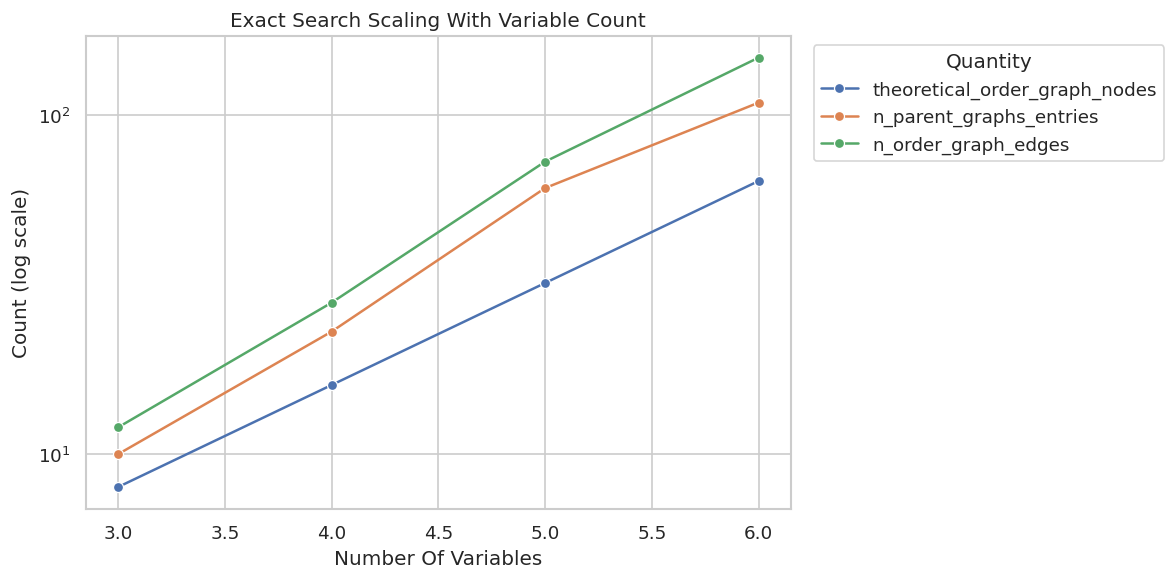
Plot Scaling Diagnostics

A plot makes the growth pattern easier to see. The y-axis is log-scaled because combinatorial quantities grow quickly.

# Plot exact-search scaling diagnostics.
scaling_plot = variable_scaling.melt(
    id_vars="variable_count",
    value_vars=["theoretical_order_graph_nodes", "n_parent_graphs_entries", "n_order_graph_edges"],
    var_name="quantity",
    value_name="count",
)
fig, ax = plt.subplots(figsize=(10, 5))
sns.lineplot(data=scaling_plot, x="variable_count", y="count", hue="quantity", marker="o", ax=ax)
ax.set_yscale("log")
ax.set_title("Exact Search Scaling With Variable Count")
ax.set_xlabel("Number Of Variables")
ax.set_ylabel("Count (log scale)")
ax.legend(title="Quantity", bbox_to_anchor=(1.02, 1), loc="upper left")
plt.tight_layout()
fig.savefig(FIGURE_DIR / f"{NOTEBOOK_PREFIX}_variable_count_scaling.png", dpi=160, bbox_inches="tight")
plt.show()

The plot shows why exact search is educational but not always operational. It gives a global optimum for the score, but the search space grows very quickly.

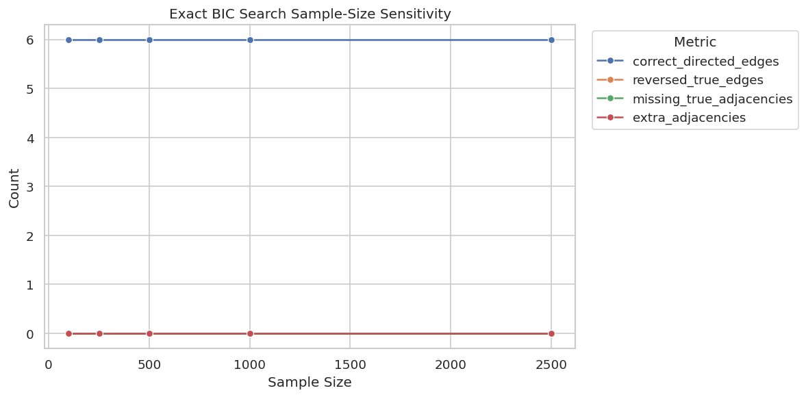
Sample-Size Sensitivity

Exact search optimizes the score for the available data. With smaller samples, local scores are noisier, so the optimal graph for the sample can differ from the optimal graph for the full dataset.

# Run exact search on subsamples to show sample-size sensitivity.
sample_rows = []
sample_edges = []
for sample_size in [100, 250, 500, 1000, len(linear_df)]:
    sample_df = linear_df.sample(n=sample_size, random_state=909 + sample_size)
    label = f"exact_bic_n_{sample_size}"
    adjacency, edge_table, stats, elapsed = run_exact_search(
        sample_df,
        label=label,
        search_method="astar",
        max_parents=None,
    )
    metrics = summarize_against_truth(edge_table, true_edges, label)
    sample_rows.append(
        {
            "run": label,
            "sample_size": sample_size,
            "elapsed_seconds": elapsed,
            "exact_bic_score_lower_is_better": total_exact_bic_score(sample_df.to_numpy(), adjacency),
            "learned_edge_count": int(adjacency.sum()),
            **stats,
            **metrics.iloc[0].drop(labels=["run"]).to_dict(),
        }
    )
    sample_edges.append(edge_table.assign(sample_size=sample_size))

sample_sensitivity = pd.DataFrame(sample_rows)
sample_sensitivity_edges = pd.concat(sample_edges, ignore_index=True)
sample_sensitivity.to_csv(TABLE_DIR / f"{NOTEBOOK_PREFIX}_sample_size_sensitivity.csv", index=False)
sample_sensitivity_edges.to_csv(TABLE_DIR / f"{NOTEBOOK_PREFIX}_sample_size_sensitivity_edges.csv", index=False)

display(sample_sensitivity)
display(sample_sensitivity_edges.head(20))

	run	sample_size	elapsed_seconds	exact_bic_score_lower_is_better	learned_edge_count	n_parent_graphs_entries	while_iter	for_iter	n_closed	max_n_opened	learned_edges_total	definite_directed_edges	true_edges	correct_directed_edges	directed_precision	directed_recall	reversed_true_edges	unresolved_true_adjacencies	missing_true_adjacencies	extra_adjacencies
0	exact_bic_n_100	100	0.007717	-364.561088	6	76	34	115	34	20	6	6	6	6	1.0	1.0	0	0	0	0
1	exact_bic_n_250	250	0.007270	-1017.879483	6	90	35	118	35	21	6	6	6	6	1.0	1.0	0	0	0	0
2	exact_bic_n_500	500	0.008129	-1825.968281	6	93	35	118	35	21	6	6	6	6	1.0	1.0	0	0	0	0
3	exact_bic_n_1000	1000	0.009568	-4033.888730	6	98	35	118	35	20	6	6	6	6	1.0	1.0	0	0	0	0
4	exact_bic_n_2500	2500	0.014748	-9950.952924	6	109	36	120	36	20	6	6	6	6	1.0	1.0	0	0	0	0

	run	source	edge_type	target	sample_size
0	exact_bic_n_100	need	-->	match	100
1	exact_bic_n_100	intent	-->	match	100
2	exact_bic_n_100	intent	-->	renewal	100
3	exact_bic_n_100	match	-->	engagement	100
4	exact_bic_n_100	engagement	-->	renewal	100
5	exact_bic_n_100	engagement	-->	support	100
6	exact_bic_n_250	need	-->	match	250
7	exact_bic_n_250	intent	-->	match	250
8	exact_bic_n_250	intent	-->	renewal	250
9	exact_bic_n_250	match	-->	engagement	250
10	exact_bic_n_250	engagement	-->	renewal	250
11	exact_bic_n_250	engagement	-->	support	250
12	exact_bic_n_500	need	-->	match	500
13	exact_bic_n_500	intent	-->	match	500
14	exact_bic_n_500	intent	-->	renewal	500
15	exact_bic_n_500	match	-->	engagement	500
16	exact_bic_n_500	engagement	-->	renewal	500
17	exact_bic_n_500	engagement	-->	support	500
18	exact_bic_n_1000	need	-->	match	1000
19	exact_bic_n_1000	intent	-->	match	1000

The sample-size table shows that an exact optimizer can still produce sample-specific graphs. Exactness refers to optimizing the score for the observed sample, not to recovering causal truth regardless of data quality.

Plot Sample-Size Sensitivity

The sample-size plot shows whether recovery improves as the number of rows grows. This is the same diagnostic logic used in earlier notebooks, now applied to exact search.

# Plot sample-size sensitivity for exact BIC search.
sample_plot = sample_sensitivity.melt(
    id_vars=["run", "sample_size"],
    value_vars=["correct_directed_edges", "reversed_true_edges", "missing_true_adjacencies", "extra_adjacencies"],
    var_name="metric",
    value_name="count",
)
fig, ax = plt.subplots(figsize=(10, 5))
sns.lineplot(data=sample_plot, x="sample_size", y="count", hue="metric", marker="o", ax=ax)
ax.set_title("Exact BIC Search Sample-Size Sensitivity")
ax.set_xlabel("Sample Size")
ax.set_ylabel("Count")
ax.legend(title="Metric", bbox_to_anchor=(1.02, 1), loc="upper left")
plt.tight_layout()
fig.savefig(FIGURE_DIR / f"{NOTEBOOK_PREFIX}_sample_size_sensitivity.png", dpi=160, bbox_inches="tight")
plt.show()

The plot separates algorithmic optimality from statistical reliability. The optimizer is exact, but the score estimate becomes more reliable as sample size grows.

Score Comparison Across Candidate Graphs

This final score diagnostic compares several candidate graphs under the same exact BIC scoring function. Lower scores are better. This helps students see that exact search is choosing among graphs by total decomposable score.

# Compare total exact BIC scores for several candidate graphs.
empty_adjacency = np.zeros((len(VARIABLES), len(VARIABLES)))
true_adjacency = edge_table_to_adjacency(true_edge_table, VARIABLES)
exact_adjacency = edge_table_to_adjacency(exact_astar_edges, VARIABLES)
ges_adjacency = edge_table_to_adjacency(ges_edges, VARIABLES)

# A deliberately incomplete candidate that omits engagement -> renewal.
incomplete_adjacency = true_adjacency.copy()
incomplete_adjacency[VARIABLES.index("engagement"), VARIABLES.index("renewal")] = 0

candidate_scores = pd.DataFrame(
    [
        {"candidate_graph": "empty_graph", "edge_count": int(empty_adjacency.sum()), "exact_bic_score_lower_is_better": total_exact_bic_score(linear_df.to_numpy(), empty_adjacency)},
        {"candidate_graph": "true_graph", "edge_count": int(true_adjacency.sum()), "exact_bic_score_lower_is_better": total_exact_bic_score(linear_df.to_numpy(), true_adjacency)},
        {"candidate_graph": "exact_search_graph", "edge_count": int(exact_adjacency.sum()), "exact_bic_score_lower_is_better": total_exact_bic_score(linear_df.to_numpy(), exact_adjacency)},
        {"candidate_graph": "ges_graph", "edge_count": int(ges_adjacency.sum()), "exact_bic_score_lower_is_better": total_exact_bic_score(linear_df.to_numpy(), ges_adjacency)},
        {"candidate_graph": "incomplete_true_graph", "edge_count": int(incomplete_adjacency.sum()), "exact_bic_score_lower_is_better": total_exact_bic_score(linear_df.to_numpy(), incomplete_adjacency)},
    ]
).sort_values("exact_bic_score_lower_is_better")

candidate_scores.to_csv(TABLE_DIR / f"{NOTEBOOK_PREFIX}_candidate_graph_score_comparison.csv", index=False)
display(candidate_scores)

	candidate_graph	edge_count	exact_bic_score_lower_is_better
1	true_graph	6	-9.950953e+03
2	exact_search_graph	6	-9.950953e+03
3	ges_graph	6	-9.950953e+03
4	incomplete_true_graph	5	-9.273215e+03
0	empty_graph	0	-1.665335e-12

The exact-search graph has the best score among these candidates. In this synthetic case it matches the true graph, but in real data the best-scoring graph should still be treated as a score-optimal candidate under assumptions.

Exact Search Reporting Checklist

The checklist below turns the notebook into reusable guidance. Exact search can sound definitive, so reporting needs to make clear what is exact and what is still assumption-dependent.

# Save a practical checklist for exact score-based discovery reports.
reporting_checklist = pd.DataFrame(
    [
        {
            "topic": "score definition",
            "question_to_answer": "Which score was optimized, and what assumptions does it make?",
            "reporting_note": "Exact search is exact for the chosen score, not for all possible causal criteria.",
        },
        {
            "topic": "search method",
            "question_to_answer": "Was A*, dynamic programming, or another exact method used?",
            "reporting_note": "Different exact methods should agree on the optimum under the same constraints.",
        },
        {
            "topic": "search-space constraints",
            "question_to_answer": "Were super-structures, required edges, or max-parent limits used?",
            "reporting_note": "Valid constraints can help; invalid constraints can force the wrong optimum.",
        },
        {
            "topic": "scaling",
            "question_to_answer": "How many variables were searched, and what were the parent-graph/order-graph statistics?",
            "reporting_note": "Exact search becomes expensive quickly as variable count grows.",
        },
        {
            "topic": "sample reliability",
            "question_to_answer": "Does the exact optimum stabilize as sample size changes?",
            "reporting_note": "The optimizer can be exact even when the sample score is noisy.",
        },
        {
            "topic": "claim strength",
            "question_to_answer": "Which edges are score-optimal candidates rather than confirmed causal facts?",
            "reporting_note": "A best-scoring DAG still needs assumptions, domain review, and sensitivity checks.",
        },
    ]
)
reporting_checklist.to_csv(TABLE_DIR / f"{NOTEBOOK_PREFIX}_exact_search_reporting_checklist.csv", index=False)
display(reporting_checklist)

	topic	question_to_answer	reporting_note
0	score definition	Which score was optimized, and what assumption...	Exact search is exact for the chosen score, no...
1	search method	Was A*, dynamic programming, or another exact ...	Different exact methods should agree on the op...
2	search-space constraints	Were super-structures, required edges, or max-...	Valid constraints can help; invalid constraint...
3	scaling	How many variables were searched, and what wer...	Exact search becomes expensive quickly as vari...
4	sample reliability	Does the exact optimum stabilize as sample siz...	The optimizer can be exact even when the sampl...
5	claim strength	Which edges are score-optimal candidates rathe...	A best-scoring DAG still needs assumptions, do...

The checklist preserves the main lesson. Exact search is a powerful benchmark for small graphs, but it does not remove the need to document scores, constraints, scaling limits, and uncertainty.

Artifact Manifest

The final cell lists the files created by this notebook so the generated figures and tables are easy to find later.

# Inventory artifacts generated by this notebook.
artifact_rows = []
for folder, artifact_type in [(TABLE_DIR, "table"), (FIGURE_DIR, "figure")]:
    for artifact_path in sorted(folder.glob(f"{NOTEBOOK_PREFIX}_*")):
        artifact_rows.append(
            {
                "artifact_type": artifact_type,
                "file_name": artifact_path.name,
                "relative_path": str(artifact_path.relative_to(NOTEBOOK_DIR)),
                "size_kb": round(artifact_path.stat().st_size / 1024, 1),
            }
        )

artifact_manifest = pd.DataFrame(artifact_rows)
artifact_manifest.to_csv(TABLE_DIR / f"{NOTEBOOK_PREFIX}_artifact_manifest.csv", index=False)
display(artifact_manifest)

	artifact_type	file_name	relative_path	size_kb
0	table	09_candidate_graph_score_comparison.csv	outputs/tables/09_candidate_graph_score_compar...	0.2
1	table	09_exact_search_concept_map.csv	outputs/tables/09_exact_search_concept_map.csv	0.8
2	table	09_exact_search_edges.csv	outputs/tables/09_exact_search_edges.csv	0.5
3	table	09_exact_search_metrics.csv	outputs/tables/09_exact_search_metrics.csv	0.3
4	table	09_exact_search_reporting_checklist.csv	outputs/tables/09_exact_search_reporting_check...	1.0
5	table	09_exact_search_stats.csv	outputs/tables/09_exact_search_stats.csv	0.3
6	table	09_exact_vs_ges_metrics.csv	outputs/tables/09_exact_vs_ges_metrics.csv	0.3
7	table	09_exact_vs_ges_score_comparison.csv	outputs/tables/09_exact_vs_ges_score_compariso...	0.1
8	table	09_forward_tier_super_graph_edges.csv	outputs/tables/09_forward_tier_super_graph_edg...	0.3
9	table	09_ges_comparison_edges.csv	outputs/tables/09_ges_comparison_edges.csv	0.3
10	table	09_loaded_dataset_summary.csv	outputs/tables/09_loaded_dataset_summary.csv	0.1
11	table	09_match_parent_set_scores.csv	outputs/tables/09_match_parent_set_scores.csv	1.4
12	table	09_max_parent_comparison.csv	outputs/tables/09_max_parent_comparison.csv	0.8
13	table	09_max_parent_edges.csv	outputs/tables/09_max_parent_edges.csv	1.1
14	table	09_package_versions.csv	outputs/tables/09_package_versions.csv	0.1
15	table	09_parent_graph_entry_summary.csv	outputs/tables/09_parent_graph_entry_summary.csv	1.4
16	table	09_sample_size_sensitivity.csv	outputs/tables/09_sample_size_sensitivity.csv	0.8
17	table	09_sample_size_sensitivity_edges.csv	outputs/tables/09_sample_size_sensitivity_edge...	1.2
18	table	09_super_graph_comparison.csv	outputs/tables/09_super_graph_comparison.csv	0.6
19	table	09_too_strict_super_graph_edges.csv	outputs/tables/09_too_strict_super_graph_edges...	0.3
20	table	09_variable_count_scaling.csv	outputs/tables/09_variable_count_scaling.csv	0.3
21	figure	09_exact_bic_astar_graph.png	outputs/figures/09_exact_bic_astar_graph.png	65.2
22	figure	09_exact_vs_ges_metrics.png	outputs/figures/09_exact_vs_ges_metrics.png	81.0
23	figure	09_sample_size_sensitivity.png	outputs/figures/09_sample_size_sensitivity.png	60.3
24	figure	09_true_dag.png	outputs/figures/09_true_dag.png	60.9
25	figure	09_variable_count_scaling.png	outputs/figures/09_variable_count_scaling.png	98.1

This notebook now has a complete exact-search workflow: BIC exact search with A* and DP, local parent-set scoring, parent-graph diagnostics, exact-vs-GES comparison, super-structure and max-parent constraints, scaling checks, sample-size sensitivity, candidate graph scoring, and reporting artifacts. The next tutorial can move into LiNGAM, where non-Gaussianity helps orient causal directions that Markov-equivalence methods may leave ambiguous.