causal-learn Tutorial 04: PC Algorithm For Continuous Data
This notebook runs the PC algorithm on the continuous synthetic data created earlier in the tutorial series. PC is a constraint-based causal discovery algorithm: it starts with a dense undirected graph, removes edges when conditional independence tests find separating sets, and then applies orientation rules to identify arrows that are supported by the discovered independence structure.
The most important lesson is that PC does not simply draw arrows from correlations. It uses many local conditional independence decisions. That means the final graph depends on:
the conditional independence test family;
the alpha threshold used for independence decisions;
sample size;
whether the algorithm’s assumptions are close enough to the data-generating process;
whether the graph is identifiable from observational data.
Here we use linear_gaussian, the friendliest dataset from notebook 02, because it matches Fisher-Z assumptions. Then we deliberately vary alpha, sample size, stable versus original PC behavior, and nonlinear data to see where the graph becomes less reliable.
Notebook Flow
We will keep the workflow close to how a real causal discovery analysis should be presented:
Set up imports, paths, and causal-learn PC utilities.
Load the continuous synthetic dataset and its known true DAG.
Review the PC assumptions and algorithm stages.
Run baseline stable PC with Fisher-Z.
Convert the learned graph into readable edge tables and figures.
Evaluate skeleton recovery and arrow recovery against the true graph.
Inspect separating sets and the raw graph matrix.
Study alpha sensitivity, sample size sensitivity, and stable PC behavior.
Stress-test Fisher-Z PC on nonlinear continuous data.
Close with reporting guidance and an artifact manifest.
The notebook is intentionally detailed because PC is one of the core algorithms that many later causal discovery methods build on or compare against.
PC Algorithm Theory
The PC algorithm is a constraint-based causal discovery method. Instead of assigning a score to each graph, it asks a sequence of conditional independence questions and uses the answers to remove edges and orient the remaining structure.
The core idea is: if two variables are independent after conditioning on some set of other variables, then they probably do not need a direct edge between them in the causal graph. PC starts with a complete undirected graph, removes edges when it finds separating sets, and then applies orientation rules to convert as many remaining edges as possible into directed edges.
PC is best understood as a graph-recovery procedure under assumptions. It is not a generic correlation screening method. The conditional independence tests, the significance level, the sample size, and the assumptions about hidden variables all shape the final graph.
Markov, Faithfulness, And Causal Sufficiency
PC relies on three major assumptions.
The causal Markov condition says that each variable is independent of its non-effects after conditioning on its direct causes. In a DAG, this is what lets graphical separation imply statistical independence.
Faithfulness says the reverse is also reliable: the independencies we see in data are exactly the independencies implied by the graph. If two causal paths cancel each other numerically, the data might show independence even though a causal path exists. That kind of cancellation breaks faithfulness and can mislead PC.
Causal sufficiency says there are no unobserved common causes among the measured variables. Standard PC assumes that if two observed variables are associated, the explanation is inside the observed variable set. If a hidden confounder drives both variables, PC may draw an ordinary edge where a latent-confounding representation would be more honest.
Skeleton Discovery And Separating Sets
PC begins with every variable connected to every other variable. Then it searches for conditioning sets that make pairs independent.
For example, if need and engagement are associated marginally, PC may initially keep an edge. But if need becomes independent of engagement after conditioning on match, then match is a separating variable and the direct need -- engagement edge can be removed.
The set that makes two variables independent is called a separating set or sepset. PC stores these sepsets because they are needed later for collider orientation. Skeleton discovery is therefore not just edge deletion; it also builds the evidence used by the orientation phase.
The search becomes harder as conditioning sets get larger. With limited data, high-order conditional independence tests are noisy, so PC can make early mistakes that propagate into later orientations.
Collider Orientation And Meek Rules
After skeleton discovery, PC looks for unshielded triples: patterns like X - Z - Y where X and Y are not adjacent. If Z was not in the separating set for X and Y, PC orients the triple as a collider:
\[
X \rightarrow Z \leftarrow Y
\]
This matters because colliders create a distinctive independence pattern. The parents of a collider can be marginally independent but become dependent after conditioning on the collider or its descendants.
After colliders are oriented, PC applies propagation rules often called Meek rules. These rules orient additional edges when doing so is logically forced by already oriented structures and the requirement that the graph remain acyclic. The algorithm orients only what is compelled; it should not invent directions where the data and rules do not support them.
CPDAGs And Markov Equivalence
PC usually returns a partially directed graph rather than a fully directed DAG. This is expected. Many DAGs can imply the same set of conditional independencies; such DAGs belong to the same Markov equivalence class.
A CPDAG represents that equivalence class. Directed edges are compelled: every DAG in the equivalence class agrees on that direction. Undirected edges are reversible: the available conditional independence information does not determine their direction.
This is why a PC result should not be judged only by whether every arrow matches a hidden truth graph. If an edge is genuinely not identifiable from observational conditional independencies, leaving it unoriented is more honest than forcing a direction.
Fisher-Z Tests For Continuous Data
In this notebook, PC uses the Fisher-Z conditional independence test. Fisher-Z is natural for continuous linear Gaussian settings because it tests whether the partial correlation between two variables is zero after conditioning on a set.
The significance level alpha controls the edge-removal threshold. A larger alpha makes it easier to reject independence, which tends to keep more edges. A smaller alpha makes independence easier to accept, which tends to remove more edges.
This means alpha is not a cosmetic setting. It changes the graph. A responsible PC workflow reports the independence test, the alpha value, sample size, and sensitivity to alpha.
What PC Can And Cannot Claim
PC can recover a CPDAG under strong assumptions and reliable conditional independence tests. It can identify some compelled directions, especially colliders, and it can reveal which adjacencies are supported by conditional dependence patterns.
PC cannot guarantee a fully directed causal graph from observational data alone. It is also vulnerable to hidden confounders, selection bias, measurement error, faithfulness violations, and weak sample sizes. In continuous data, nonlinear relationships can also make a linear Fisher-Z test miss important dependencies.
The practical lesson is to read PC output as a structured causal hypothesis. The graph is strongest when assumptions are plausible, directions are stable across settings, and the result agrees with domain constraints or complementary methods.
Setup
The setup cell imports the scientific stack, the PC algorithm, and causal-learn’s graph metrics. It also prepares output folders and records package versions. The MPLCONFIGDIR setting keeps matplotlib cache files inside the repository workspace during notebook execution.
The version table is the reproducibility anchor for the notebook. Graph outputs can change when packages, random seeds, or tuning choices change, so the environment should be visible next to the results.
Load Continuous Data And Ground Truth
This notebook uses 02_linear_gaussian.csv from the synthetic data factory. That dataset was designed to be friendly to Fisher-Z PC: continuous variables, linear additive structural equations, Gaussian noise, and no hidden common causes in the observed graph.
We also load the true edge table so the learned graph can be evaluated honestly.
Both datasets have the same observed columns. The baseline PC run will use the linear Gaussian data; the nonlinear dataset appears later as a stress test for what happens when Fisher-Z assumptions are less appropriate.
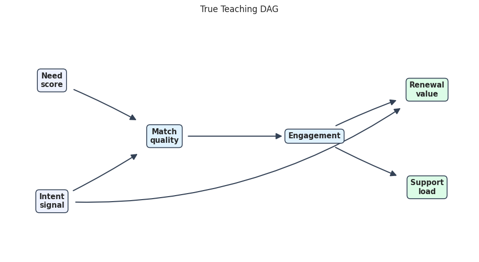
True DAG Edge Table
The true edge table is the answer key. PC should try to recover the adjacency pattern and, where identifiable, the orientations implied by the conditional independence structure.
Engagement creates more chances for support contact.
-->
This edge table is intentionally small. With only six variables, we can inspect every learned edge by hand and understand exactly what each graph metric is counting.
PC Assumptions And Stages
PC is powerful, but its output is only as credible as its assumptions. This table summarizes the conceptual contract for the baseline run.
pc_assumption_table = pd.DataFrame( [ {"assumption_or_stage": "Causal Markov condition","plain_language": "The graph implies the conditional independences in the data.","why_it_matters": "PC removes edges using conditional independence tests.", }, {"assumption_or_stage": "Faithfulness","plain_language": "Independences in the data are explained by the graph, not by exact coefficient cancellations.","why_it_matters": "If faithfulness fails, PC can remove or keep the wrong edges.", }, {"assumption_or_stage": "Causal sufficiency","plain_language": "All common causes of observed variables are included.","why_it_matters": "PC targets a DAG/CPDAG under observed sufficiency; FCI is safer with hidden common causes.", }, {"assumption_or_stage": "Correct CI test","plain_language": "Fisher-Z is appropriate for approximately linear Gaussian continuous data.","why_it_matters": "A mismatched test can create false edge deletions or false retained edges.", }, {"assumption_or_stage": "Skeleton search","plain_language": "Start dense, then remove edges when separating sets are found.","why_it_matters": "This controls which variable pairs remain adjacent.", }, {"assumption_or_stage": "Orientation rules","plain_language": "Orient colliders and propagate directions without introducing cycles or contradictions.","why_it_matters": "Some directions are identifiable, while others may remain undirected.", }, ])pc_assumption_table.to_csv(TABLE_DIR /f"{NOTEBOOK_PREFIX}_pc_assumptions_and_stages.csv", index=False)pc_assumption_table
assumption_or_stage
plain_language
why_it_matters
0
Causal Markov condition
The graph implies the conditional independences in the data.
PC removes edges using conditional independence tests.
1
Faithfulness
Independences in the data are explained by the graph, not by exact coefficient cancellations.
If faithfulness fails, PC can remove or keep the wrong edges.
2
Causal sufficiency
All common causes of observed variables are included.
PC targets a DAG/CPDAG under observed sufficiency; FCI is safer with hidden common causes.
3
Correct CI test
Fisher-Z is appropriate for approximately linear Gaussian continuous data.
A mismatched test can create false edge deletions or false retained edges.
4
Skeleton search
Start dense, then remove edges when separating sets are found.
This controls which variable pairs remain adjacent.
5
Orientation rules
Orient colliders and propagate directions without introducing cycles or contradictions.
Some directions are identifiable, while others may remain undirected.
This checklist is the right frame for reading every PC graph below. A clean graph recovery result on synthetic linear Gaussian data does not mean the same settings will work on nonlinear, discrete, missing, or hidden-confounder data.
Data Audit Before Running PC
Before running discovery, we check basic shape, missingness, and summary statistics. This dataset is synthetic, but the audit habit matters: PC can be sensitive to missingness, nonnumeric columns, duplicated columns, and extreme scaling problems.
The variables are numeric, complete, centered, and scaled. That makes the baseline PC result easier to attribute to graph structure rather than messy data preparation issues.
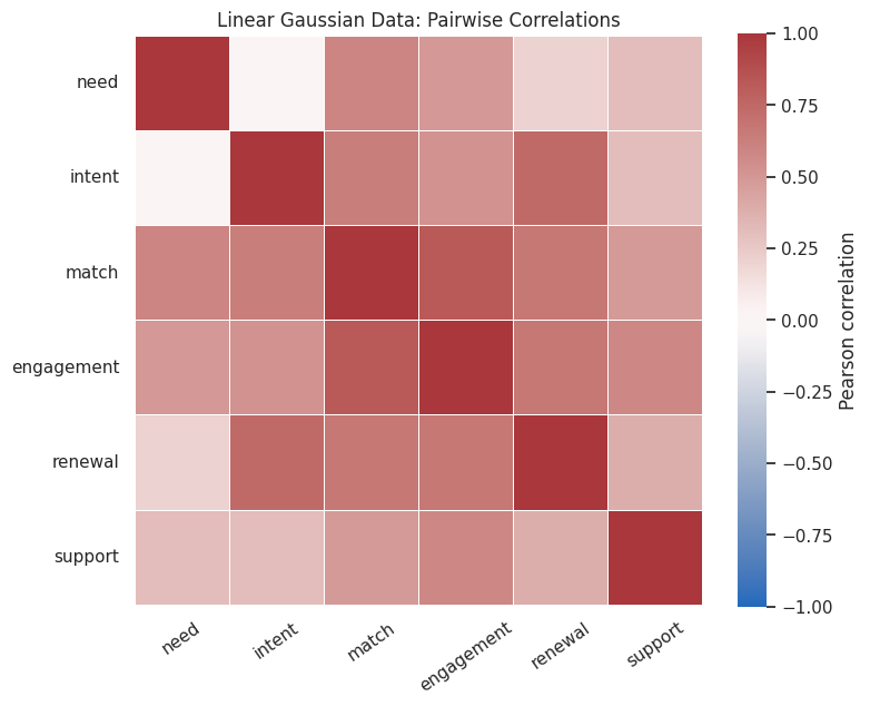
Correlation Map Before Conditional Testing
A correlation heatmap is not a causal graph, but it is a useful first diagnostic. It shows which variables are associated before PC starts conditioning on other variables to remove indirect relationships.
Many non-adjacent variables are correlated because causal paths transmit association. PC’s job is to decide which of these pairwise associations disappear after conditioning on appropriate separating sets.
Graph Conversion And Drawing Helpers
The PC output is a causal-learn graph object. The helper functions below convert that object into readable edge tables, compute graph metrics, and draw graphs in the same visual style used across the tutorial.
The evaluation separates skeleton recovery from arrow recovery. This distinction matters because PC may correctly keep two variables adjacent while leaving the direction unresolved or orienting it incorrectly under finite-sample noise.
Drawing Helper For DAG-Style Graphs
This renderer uses the shared tutorial visual style: wide canvas, rounded pastel boxes, bold labels, dark arrows, and enough spacing that arrowheads are visible. Undirected CPDAG-style edges are drawn as solid lines without arrowheads.
The true graph figure is the visual baseline for the rest of the notebook. Each learned PC graph can be compared against this layout without mentally rearranging variables.
Run Baseline Stable PC
The baseline run uses settings that match the synthetic data:
indep_test="fisherz" for continuous linear Gaussian-style data;
alpha=0.05 as the conditional-independence threshold;
stable=True so skeleton discovery is less sensitive to variable order.
The result is a causal-learn CausalGraph object containing a learned graph and separating-set information.
The baseline learned edge table is already very close to the true edge table. Because this dataset was designed for Fisher-Z PC, this is the friendly case where the algorithm’s assumptions and the data-generating process are aligned.
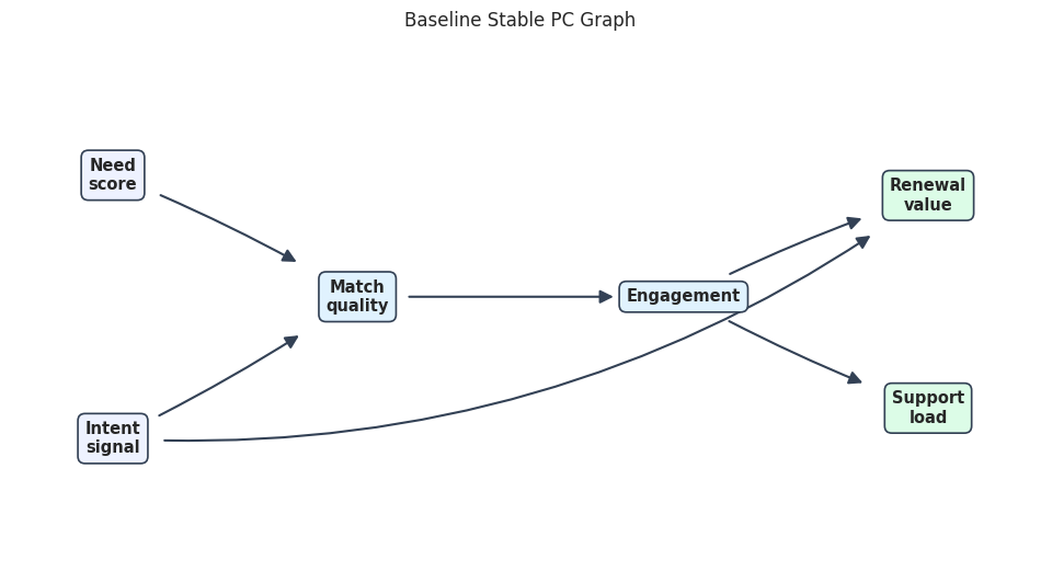
Baseline Learned Graph
The next figure draws the learned graph using the same positions as the true DAG. Matching positions make extra, missing, reversed, or unresolved edges easier to see.
baseline_graph_path = FIGURE_DIR /f"{NOTEBOOK_PREFIX}_baseline_pc_graph.png"draw_edge_table_graph(baseline_edge_table, "Baseline Stable PC Graph", baseline_graph_path)
The learned graph matches the intended structure in this synthetic baseline. This clean result is useful because we can now perturb the settings and see how the same algorithm becomes less stable.
Evaluate Baseline Graph Recovery
Because the true graph is known, we can score the learned graph. Skeleton metrics ask whether the right variable pairs are connected. Arrow metrics ask whether the directed claims match the true directions.
The baseline metrics are high because the data were intentionally friendly. This should not be read as proof that PC will always recover the true graph; it shows that the implementation and synthetic setup are working as expected.
causal-learn Built-In Metrics
The custom metric table is easy to read, but causal-learn also provides graph comparison utilities. This cell builds a true Dag object and compares it with the baseline PC output using SHD, adjacency confusion, and arrow confusion.
The built-in metrics agree with the custom recovery table. In larger experiments, built-in metrics are convenient, while custom edge tables remain useful for explaining exactly which edge changed.
Inspect The Raw Graph Matrix
causal-learn stores endpoint information in a graph matrix. The encoding is compact but not especially friendly for reporting. We keep it here because it helps connect the readable edge strings to the underlying object representation.
The matrix is useful for debugging and programmatic conversion, but the edge table is safer for communication. A report should not assume readers know causal-learn’s internal endpoint codes.
Separating Sets Found By PC
When PC removes an edge, it stores a separating set: a set of variables that made the pair conditionally independent. Separating sets are the bridge between local CI-test decisions and the final skeleton.
def format_sepset_entry(entry, names):"""Convert one causal-learn sepset entry into readable variable names."""if entry isNone:return"none recorded" formatted_sets = []for conditioning_set in entry:iflen(conditioning_set) ==0: formatted_sets.append("empty set")else: formatted_sets.append("{"+", ".join(names[int(index)] for index in conditioning_set) +"}")return"; ".join(dict.fromkeys(formatted_sets))learned_skeleton = skeleton_edges(baseline_edge_table)sepset_rows = []for i, x inenumerate(node_order):for j, y inenumerate(node_order):if i >= j:continueiffrozenset([x, y]) in learned_skeleton:continue sepset_rows.append( {"x": x,"y": y,"separating_sets": format_sepset_entry(baseline_pc.sepset[i][j], node_order), } )separating_sets = pd.DataFrame(sepset_rows)separating_sets.to_csv(TABLE_DIR /f"{NOTEBOOK_PREFIX}_baseline_separating_sets.csv", index=False)separating_sets
x
y
separating_sets
0
need
intent
empty set
1
need
engagement
{match}
2
need
renewal
{intent, match, engagement}
3
need
support
{match, engagement}
4
intent
engagement
{match}
5
intent
support
{match, engagement}
6
match
renewal
{intent, engagement}
7
match
support
{engagement}
8
renewal
support
{engagement}
The separating sets explain why non-adjacent pairs were removed. For example, a downstream association can disappear after conditioning on variables along the path. This is the operational heart of PC.
Alpha Sensitivity
The alpha value controls how easily PC rejects conditional independence. A higher alpha rejects independence more often, which tends to keep more edges. A lower alpha accepts independence more readily, which can remove edges more aggressively.
This cell runs PC across several alpha values and evaluates each learned graph against the true DAG.
def run_pc_edge_table(dataframe, alpha=BASE_ALPHA, stable=True, sample_size=None, random_state=RANDOM_SEED):"""Run PC on a dataframe and return the causal graph plus a readable edge table."""if sample_size isnotNone: run_data = dataframe[node_order].sample(n=sample_size, random_state=random_state)else: run_data = dataframe[node_order] result = pc( run_data.to_numpy(), alpha=alpha, indep_test="fisherz", stable=stable, show_progress=False, node_names=node_order, ) edge_table = graph_to_edge_table(result.G)return result, edge_tablealpha_values = [0.001, 0.005, 0.01, 0.05, 0.10, 0.20]alpha_rows = []alpha_edge_rows = []for alpha in alpha_values: result, edge_table = run_pc_edge_table(linear_data, alpha=alpha, stable=True) metrics = evaluate_learned_graph(f"alpha_{alpha}", true_edge_table, edge_table) metrics["alpha"] = alpha metrics["edge_list"] ="; ".join(edge_table["causal_learn_edge"].tolist()) alpha_rows.append(metrics)for row in edge_table.itertuples(index=False): alpha_edge_rows.append({"alpha": alpha, **row._asdict()})alpha_sensitivity = pd.DataFrame(alpha_rows)alpha_edge_table = pd.DataFrame(alpha_edge_rows)alpha_sensitivity.to_csv(TABLE_DIR /f"{NOTEBOOK_PREFIX}_alpha_sensitivity_metrics.csv", index=False)alpha_edge_table.to_csv(TABLE_DIR /f"{NOTEBOOK_PREFIX}_alpha_sensitivity_edges.csv", index=False)alpha_sensitivity[ ["alpha","learned_edges","skeleton_precision","skeleton_recall","arrow_precision","arrow_recall","reversed_arrows","unresolved_true_edges","edge_list", ]]
alpha
learned_edges
skeleton_precision
skeleton_recall
arrow_precision
arrow_recall
reversed_arrows
unresolved_true_edges
edge_list
0
0.001
6
1.00
1.0
1.0
1.000000
0
0
engagement --> renewal; engagement --> support; intent --> match; intent --> renewal; match --> engagement; need --> match
1
0.005
6
1.00
1.0
1.0
1.000000
0
0
engagement --> renewal; engagement --> support; intent --> match; intent --> renewal; match --> engagement; need --> match
2
0.010
6
1.00
1.0
1.0
1.000000
0
0
engagement --> renewal; engagement --> support; intent --> match; intent --> renewal; match --> engagement; need --> match
3
0.050
6
1.00
1.0
1.0
1.000000
0
0
engagement --> renewal; engagement --> support; intent --> match; intent --> renewal; match --> engagement; need --> match
4
0.100
6
1.00
1.0
1.0
1.000000
0
0
engagement --> renewal; engagement --> support; intent --> match; intent --> renewal; match --> engagement; need --> match
Most moderate alpha values recover the same graph in this friendly dataset. The high-alpha run keeps too many relationships and begins to distort orientations. This is exactly why a graph should not be reported at one threshold without sensitivity checks.
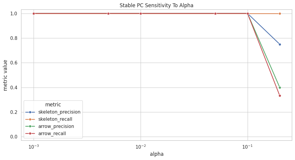
Plot Alpha Sensitivity
The next plot tracks skeleton and arrow quality as alpha changes. Skeleton metrics focus on adjacency recovery; arrow metrics focus on direction recovery.
The plot stays flat until alpha becomes very permissive. That is a good sign for this synthetic dataset, but the high-alpha deterioration is a useful warning: tuning choices can change causal claims.
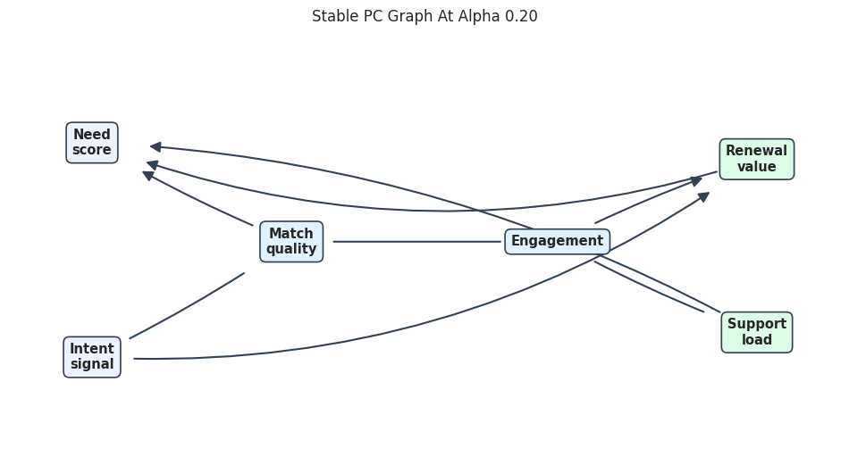
Draw The High-Alpha Graph
The alpha sensitivity table showed that alpha=0.20 produces a less reliable graph. Drawing that graph makes the error mode easier to see.
high_alpha_result, high_alpha_edge_table = run_pc_edge_table(linear_data, alpha=0.20, stable=True)high_alpha_edge_table.to_csv(TABLE_DIR /f"{NOTEBOOK_PREFIX}_high_alpha_edges.csv", index=False)high_alpha_graph_path = FIGURE_DIR /f"{NOTEBOOK_PREFIX}_high_alpha_pc_graph.png"draw_edge_table_graph(high_alpha_edge_table, "Stable PC Graph At Alpha 0.20", high_alpha_graph_path)high_alpha_edge_table
source
target
mark
edge_kind
causal_learn_edge
endpoint_at_node1
endpoint_at_node2
0
engagement
renewal
-->
directed
engagement --> renewal
TAIL
ARROW
1
engagement
support
---
undirected
engagement --- support
TAIL
TAIL
2
intent
match
---
undirected
intent --- match
TAIL
TAIL
3
intent
renewal
-->
directed
intent --> renewal
TAIL
ARROW
4
match
engagement
---
undirected
match --- engagement
TAIL
TAIL
5
match
need
-->
directed
match --> need
TAIL
ARROW
6
renewal
need
-->
directed
renewal --> need
TAIL
ARROW
7
support
need
-->
directed
support --> need
TAIL
ARROW
The high-alpha graph contains extra or misoriented relationships that the baseline graph avoided. The lesson is practical: alpha is not a cosmetic parameter; it changes the graph search decisions.
Sample Size Sensitivity
Finite samples can make conditional independence tests unstable. The next experiment repeatedly samples smaller subsets of the same linear Gaussian data and runs stable PC with alpha=0.05.
engagement --> support; intent --> match; intent --- renewal; match --> engagement; need --> match; renewal --> engagement
1
150
5
1.0
0.833333
1.0
0.666667
0
1
engagement --> support; intent --> match; intent --- renewal; match --> engagement; need --> match
2
250
6
1.0
1.000000
0.6
0.500000
2
1
intent --> match; intent --- renewal; match --> engagement; need --> match; renewal --> engagement; support --> engagement
3
500
6
1.0
1.000000
1.0
1.000000
0
0
engagement --> renewal; engagement --> support; intent --> match; intent --> renewal; match --> engagement; need --> match
4
1000
6
1.0
1.000000
1.0
1.000000
0
0
engagement --> renewal; engagement --> support; intent --> match; intent --> renewal; match --> engagement; need --> match
5
2500
6
1.0
1.000000
1.0
1.000000
0
0
engagement --> renewal; engagement --> support; intent --> match; intent --> renewal; match --> engagement; need --> match
The smaller samples recover the broad structure less reliably. Some directions become unresolved or reversed, while larger samples return to the intended graph. This is the finite-sample side of the CI-test story from notebook 03.
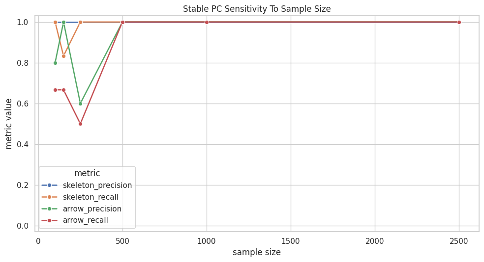
Plot Sample Size Sensitivity
This plot shows graph recovery metrics as the available sample grows. It is often one of the most useful diagnostics for explaining why a discovery graph should be treated cautiously.
The plot improves as sample size increases. Skeleton recovery is generally easier than orientation recovery, which is a common pattern in causal discovery benchmarks.
Stable PC Versus Original PC
The stable=True option makes skeleton discovery less dependent on variable ordering. This cell compares stable and original PC on moderate sample sizes where finite-sample differences can show up.
engagement --> support; intent --> match; intent --- renewal; match --> engagement; need --> match
1
True
250
6
1.0
1.000000
0.6
0.500000
intent --> match; intent --- renewal; match --> engagement; need --> match; renewal --> engagement; support --> engagement
2
True
500
6
1.0
1.000000
1.0
1.000000
engagement --> renewal; engagement --> support; intent --> match; intent --> renewal; match --> engagement; need --> match
3
False
150
5
1.0
0.833333
1.0
0.666667
engagement --> support; intent --> match; intent --- renewal; match --> engagement; need --> match
4
False
250
6
1.0
1.000000
0.6
0.500000
intent --> match; intent --- renewal; match --> engagement; need --> match; renewal --> engagement; support --> engagement
5
False
500
6
1.0
1.000000
0.6
0.500000
intent --> match; intent --- renewal; match --> engagement; need --> match; renewal --> engagement; support --> engagement
The stable and original variants can agree at some sample sizes and differ at others. Stable PC is often preferred for reproducible skeleton discovery because it reduces order-dependence during edge removal.
Stress Test: Fisher-Z PC On Nonlinear Continuous Data
The nonlinear dataset has the same broad variables but violates the linear Gaussian assumptions more strongly. Running Fisher-Z PC here is useful as a cautionary example: the algorithm still returns a graph, but the test may not match the data-generating mechanisms.
The nonlinear Fisher-Z graph is less faithful to the true base graph. This does not mean PC is useless; it means the test choice and data-generating assumptions are no longer aligned.
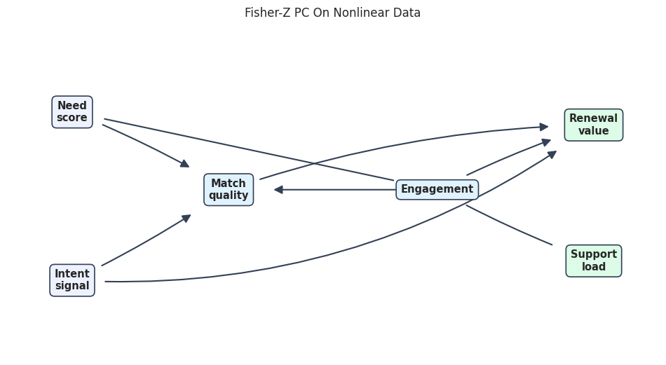
Draw The Nonlinear Stress-Test Graph
The figure shows the stress-test graph in the same layout as the baseline. This makes extra and reversed edges easier to spot.
nonlinear_graph_path = FIGURE_DIR /f"{NOTEBOOK_PREFIX}_nonlinear_fisherz_pc_graph.png"draw_edge_table_graph(nonlinear_pc_edge_table, "Fisher-Z PC On Nonlinear Data", nonlinear_graph_path)nonlinear_metrics
candidate
learned_edges
skeleton_tp
skeleton_fp
skeleton_fn
skeleton_precision
skeleton_recall
arrow_tp
arrow_fp
arrow_fn
arrow_precision
arrow_recall
reversed_arrows
unresolved_true_edges
0
nonlinear_fisherz_pc
8
6
2
0
0.75
1.0
4
2
2
0.666667
0.666667
1
1
The metrics and graph both point in the same direction: when the CI test is mismatched, PC can preserve the wrong adjacencies or orient arrows poorly. Later nonlinear-method notebooks will revisit this issue with methods designed for richer functional relationships.
Compare Baseline And Stress-Test Metrics
This compact table puts the friendly baseline, high-alpha run, small-sample run, and nonlinear stress test side by side.
The comparison shows three distinct failure modes: too-permissive alpha can add edges, small samples can weaken orientation recovery, and nonlinear mechanisms can break Fisher-Z assumptions. These are exactly the diagnostics a PC analysis should include.
Report-Ready PC Checklist
The final checklist turns this notebook into reporting guidance. A useful PC report should include the graph, the CI test, the alpha threshold, stability diagnostics, and assumption caveats.
pc_reporting_checklist = pd.DataFrame( [ {"report_item": "Data regime","example_from_this_notebook": "Continuous linear Gaussian synthetic data","why_it_matters": "Fisher-Z is only appropriate when the data are close to its assumptions.", }, {"report_item": "CI test and alpha","example_from_this_notebook": "Fisher-Z with alpha = 0.05","why_it_matters": "Edge removal depends directly on conditional independence decisions.", }, {"report_item": "Stable setting","example_from_this_notebook": "stable=True for the baseline graph","why_it_matters": "Stable PC reduces order-dependence in skeleton search.", }, {"report_item": "Graph type","example_from_this_notebook": "Learned directed/undirected graph from PC","why_it_matters": "Unoriented edges should not be silently converted into causal arrows.", }, {"report_item": "Sensitivity checks","example_from_this_notebook": "Alpha, sample size, stable versus original PC, nonlinear stress test","why_it_matters": "A single graph can hide tuning and assumption fragility.", }, {"report_item": "Edge-level audit","example_from_this_notebook": "Saved learned edge tables and separating sets","why_it_matters": "Stakeholders need to know which causal claims changed, not just a summary score.", }, ])pc_reporting_checklist.to_csv(TABLE_DIR /f"{NOTEBOOK_PREFIX}_pc_reporting_checklist.csv", index=False)pc_reporting_checklist
report_item
example_from_this_notebook
why_it_matters
0
Data regime
Continuous linear Gaussian synthetic data
Fisher-Z is only appropriate when the data are close to its assumptions.
1
CI test and alpha
Fisher-Z with alpha = 0.05
Edge removal depends directly on conditional independence decisions.
2
Stable setting
stable=True for the baseline graph
Stable PC reduces order-dependence in skeleton search.
3
Graph type
Learned directed/undirected graph from PC
Unoriented edges should not be silently converted into causal arrows.
4
Sensitivity checks
Alpha, sample size, stable versus original PC, nonlinear stress test
A single graph can hide tuning and assumption fragility.
5
Edge-level audit
Saved learned edge tables and separating sets
Stakeholders need to know which causal claims changed, not just a summary score.
The checklist is the habit to carry forward. PC is not just an API call; it is a sequence of assumptions, tests, graph edits, and sensitivity checks that need to be made visible.
Generated Artifact Manifest
The last cell lists the files created by this notebook. Downstream notebooks can reuse the edge tables, metrics, and figures when comparing PC to other discovery algorithms.
The continuous PC tutorial is now complete. The next notebook can extend the same PC workflow to prior knowledge, missing values, and discrete data, where the choice of CI test and background constraints becomes even more visible.