causal-learn Tutorial 03: Independence Tests

Constraint-based causal discovery is built on a repeated question:

Are variables X and Y independent after conditioning on a set of variables Z?

If the answer is yes, algorithms such as PC and FCI can remove or mark edges. If the answer is no, the variables remain connected under the current conditioning set. This makes conditional independence tests one of the most important pieces of the causal discovery workflow.

This notebook uses the synthetic datasets created in notebook 02. Because those datasets have known structural equations and known true graphs, we can connect each p-value to a causal pattern:

• a true direct edge should usually look dependent;
• an indirect path may become independent after conditioning on the right mediators;
• a collider can create dependence after conditioning;
• a test that matches the data type can behave very differently from a mismatched test.

The point is not to memorize p-values. The point is to learn how conditional independence tests become graph-editing decisions.

Notebook Flow

We will build the independence-testing workflow step by step:

1. Set up imports, paths, and causal-learn’s CIT interface.
2. Load the synthetic datasets and true edge tables from notebook 02.
3. Review which test belongs to which data regime.
4. Run Fisher-Z tests on the linear Gaussian dataset.
5. Study path blocking, collider opening, alpha sensitivity, sample size, and conditioning-set size.
6. Compare Fisher-Z with KCI on nonlinear dependence.
7. Run chi-square and G-square tests on the discrete dataset.
8. Use missing-value Fisher-Z on a controlled missingness example.
9. Save results and close with practical reporting guidance.

Later PC and FCI notebooks will use these same test families inside graph-search algorithms.

Setup

This cell imports the scientific stack, prepares output folders, loads causal-learn’s conditional independence test factory, and defines a few display helpers. The MPLCONFIGDIR line is set before importing matplotlib so notebook execution does not try to write cache files outside the workspace.

from pathlib import Path
from importlib.metadata import PackageNotFoundError, version
import os
import warnings

os.environ.setdefault("MPLCONFIGDIR", str(Path.cwd() / ".matplotlib_cache"))

import numpy as np
import pandas as pd
import matplotlib.pyplot as plt
import seaborn as sns

from causallearn.utils.cit import CIT

warnings.filterwarnings("ignore", category=FutureWarning)
sns.set_theme(style="whitegrid", context="notebook")
pd.set_option("display.max_columns", 120)
pd.set_option("display.max_colwidth", 140)

NOTEBOOK_DIR = Path.cwd()
if NOTEBOOK_DIR.name != "causal_learn":
    NOTEBOOK_DIR = Path("notebooks/tutorials/causal_learn").resolve()
else:
    NOTEBOOK_DIR = NOTEBOOK_DIR.resolve()

OUTPUT_DIR = NOTEBOOK_DIR / "outputs"
FIGURE_DIR = OUTPUT_DIR / "figures"
TABLE_DIR = OUTPUT_DIR / "tables"
DATASET_DIR = OUTPUT_DIR / "datasets"
REPORT_DIR = OUTPUT_DIR / "reports"
for directory in [OUTPUT_DIR, FIGURE_DIR, TABLE_DIR, DATASET_DIR, REPORT_DIR]:
    directory.mkdir(parents=True, exist_ok=True)

NOTEBOOK_PREFIX = "03"
RANDOM_SEED = 42
ALPHA = 0.05


def pkg_version(package_name: str) -> str:
    """Return a package version string without failing if package metadata is unavailable."""
    try:
        return version(package_name)
    except PackageNotFoundError:
        return "not installed"

version_table = pd.DataFrame(
    [
        {"package": "causal-learn", "version": pkg_version("causal-learn")},
        {"package": "numpy", "version": pkg_version("numpy")},
        {"package": "pandas", "version": pkg_version("pandas")},
        {"package": "matplotlib", "version": pkg_version("matplotlib")},
        {"package": "seaborn", "version": pkg_version("seaborn")},
    ]
)
version_table

	package	version
0	causal-learn	0.1.4.5
1	numpy	2.4.4
2	pandas	3.0.2
3	matplotlib	3.10.9
4	seaborn	0.13.2

The version table anchors the test behavior to a concrete environment. Conditional independence tests can have implementation details such as caching, numerical tolerances, and kernel defaults, so recording versions is a small but valuable reproducibility habit.

Load The Synthetic Datasets

Notebook 02 generated several datasets under outputs/datasets. This notebook loads the ones needed for independence-test examples:

• linear_gaussian: friendly baseline for Fisher-Z.
• nonlinear_continuous: nonlinear mechanisms where linear tests can be limited.
• discrete_mixed: binary and ordinal variables for chi-square and G-square tests.
• hidden_confounder_observed: observed-only data with an omitted common cause.

If this cell fails because a file is missing, run notebook 02 first.

dataset_paths = {
    "linear_gaussian": DATASET_DIR / "02_linear_gaussian.csv",
    "nonlinear_continuous": DATASET_DIR / "02_nonlinear_continuous.csv",
    "discrete_mixed": DATASET_DIR / "02_discrete_mixed.csv",
    "hidden_confounder_observed": DATASET_DIR / "02_hidden_confounder_observed.csv",
}

missing_files = [str(path) for path in dataset_paths.values() if not path.exists()]
if missing_files:
    raise FileNotFoundError(
        "Synthetic datasets are missing. Run notebook 02 first. Missing files: " + ", ".join(missing_files)
    )

datasets = {name: pd.read_csv(path) for name, path in dataset_paths.items()}
base_edge_table = pd.read_csv(TABLE_DIR / "02_base_true_dag_edges.csv")
variable_dictionary = pd.read_csv(TABLE_DIR / "02_variable_dictionary.csv")
base_nodes = ["need", "intent", "match", "engagement", "renewal", "support"]

loaded_summary = pd.DataFrame(
    [
        {
            "dataset_name": name,
            "rows": data.shape[0],
            "columns": data.shape[1],
            "column_list": ", ".join(data.columns),
        }
        for name, data in datasets.items()
    ]
)
loaded_summary.to_csv(TABLE_DIR / f"{NOTEBOOK_PREFIX}_loaded_dataset_summary.csv", index=False)
loaded_summary

	dataset_name	rows	columns	column_list
0	linear_gaussian	2500	6	need, intent, match, engagement, renewal, support
1	nonlinear_continuous	2500	6	need, intent, match, engagement, renewal, support
2	discrete_mixed	2500	6	need, intent, match, engagement, renewal, support
3	hidden_confounder_observed	2500	6	need, intent, match, engagement, renewal, support

The loaded datasets all have the expected observed variables. The discrete dataset uses integer-valued columns, while the continuous datasets are standardized numeric signals.

Test Selection Guide

causal-learn exposes conditional independence tests through CIT(data, method). The method choice should match the data and assumptions. A mismatched test can produce confident-looking p-values for the wrong question.

ci_test_guide = pd.DataFrame(
    [
        {
            "method_name": "fisherz",
            "data_type": "continuous",
            "main_assumption": "Approximately linear Gaussian relationships after conditioning.",
            "typical_use": "PC on continuous Gaussian-style tabular data.",
            "caution": "Can miss nonlinear dependence and can be sensitive to conditioning-set size.",
        },
        {
            "method_name": "mv_fisherz",
            "data_type": "continuous with missing values",
            "main_assumption": "Fisher-Z style test with missing-value handling.",
            "typical_use": "PC-style workflows when data have missing entries.",
            "caution": "Missingness assumptions still matter; this is not magic protection against selection bias.",
        },
        {
            "method_name": "chisq",
            "data_type": "discrete",
            "main_assumption": "Counts in contingency tables are informative enough for chi-square approximations.",
            "typical_use": "Binary or categorical discovery examples.",
            "caution": "Sparse categories and large conditioning sets can make the approximation weak.",
        },
        {
            "method_name": "gsq",
            "data_type": "discrete",
            "main_assumption": "Likelihood-ratio version of a discrete conditional independence test.",
            "typical_use": "Alternative to chi-square for categorical data.",
            "caution": "Still depends on enough observations per conditioned cell.",
        },
        {
            "method_name": "kci",
            "data_type": "continuous or mixed numeric",
            "main_assumption": "Kernel-based dependence test can detect nonlinear relationships.",
            "typical_use": "Nonlinear discovery examples and robustness checks.",
            "caution": "More computationally expensive; kernel choices and sample size matter.",
        },
    ]
)

ci_test_guide.to_csv(TABLE_DIR / f"{NOTEBOOK_PREFIX}_ci_test_selection_guide.csv", index=False)
ci_test_guide

	method_name	data_type	main_assumption	typical_use	caution
0	fisherz	continuous	Approximately linear Gaussian relationships after conditioning.	PC on continuous Gaussian-style tabular data.	Can miss nonlinear dependence and can be sensitive to conditioning-set size.
1	mv_fisherz	continuous with missing values	Fisher-Z style test with missing-value handling.	PC-style workflows when data have missing entries.	Missingness assumptions still matter; this is not magic protection against selection bias.
2	chisq	discrete	Counts in contingency tables are informative enough for chi-square approximations.	Binary or categorical discovery examples.	Sparse categories and large conditioning sets can make the approximation weak.
3	gsq	discrete	Likelihood-ratio version of a discrete conditional independence test.	Alternative to chi-square for categorical data.	Still depends on enough observations per conditioned cell.
4	kci	continuous or mixed numeric	Kernel-based dependence test can detect nonlinear relationships.	Nonlinear discovery examples and robustness checks.	More computationally expensive; kernel choices and sample size matter.

This table is the decision layer before any algorithm call. For example, using Fisher-Z on binary variables may run, but it does not mean the resulting p-values answer the intended discrete conditional-independence question.

Helper Functions For Running Tests

The CIT object expects numeric column indices, not column names. The helper below lets us write tests using variable names and conditioning-set names. It returns p-values and a plain decision at a chosen alpha level.

def make_ci_runner(dataframe, columns, method):
    """Create a named-column wrapper around causal-learn's CIT interface."""
    matrix = dataframe[columns].to_numpy()
    column_to_index = {column: position for position, column in enumerate(columns)}
    ci_test = CIT(matrix, method)

    def run_test(x, y, conditioning_set=()):
        conditioning_set = tuple(conditioning_set)
        x_idx = column_to_index[x]
        y_idx = column_to_index[y]
        z_idx = tuple(column_to_index[z] for z in conditioning_set)
        p_value = float(ci_test(x_idx, y_idx, z_idx))
        return p_value

    return run_test


def decision_from_p_value(p_value, alpha=ALPHA):
    """Translate a p-value into the graph-search decision language."""
    return "reject independence" if p_value < alpha else "do not reject independence"


def p_value_label(p_value):
    """Format tiny p-values without losing the fact that they are very small."""
    if p_value == 0:
        return "<1e-300"
    if p_value < 0.001:
        return f"{p_value:.2e}"
    return f"{p_value:.3f}"


PLOT_LOG_CAP = 20


def capped_minus_log10(values, cap=PLOT_LOG_CAP):
    """Convert p-values to -log10 scale while capping extremes for readable plots."""
    transformed = -np.log10(pd.Series(values).replace(0, np.nextafter(0, 1)))
    return transformed.clip(upper=cap)

"helpers ready"

'helpers ready'

The decision phrase mirrors constraint-based discovery. A very small p-value means the test rejects the null of conditional independence, so an algorithm would usually keep the variables connected for that conditioning set. A large p-value means the test does not reject independence, so an algorithm may remove an edge or record a separating set.

The True Edge Table

Before testing, we inspect the base true graph again. The most important thing to remember is that pairwise association does not equal a direct edge. Variables can be associated through chains, forks, or opened colliders.

base_edge_table.to_csv(TABLE_DIR / f"{NOTEBOOK_PREFIX}_base_true_edges_used.csv", index=False)
base_edge_table

	source	target	edge_type	mechanism
0	need	match	directed	Need changes what a good match means.
1	intent	match	directed	Current intent changes recommendation relevance.
2	match	engagement	directed	Better matching increases engagement depth.
3	intent	renewal	directed	Intent directly affects later value.
4	engagement	renewal	directed	Engagement contributes to renewal value.
5	engagement	support	directed	Engagement creates more chances for support contact.

The true edges define what later graph algorithms should recover. Independence tests are the local evidence used to remove impossible adjacencies and orient some structures, but each individual test only answers one local question.

Fisher-Z On Linear Gaussian Data

Fisher-Z is the friendly baseline for this tutorial because linear_gaussian was generated from linear additive equations with Gaussian noise. The test checks whether the partial correlation between two variables is zero after conditioning on a set of variables.

The cases below cover four teaching patterns:

• a direct edge that should be dependent;
• an indirect association that becomes independent after blocking paths;
• two independent roots;
• a collider that creates dependence after conditioning.

linear_runner = make_ci_runner(datasets["linear_gaussian"], base_nodes, "fisherz")

fisherz_cases = [
    {
        "case": "direct edge",
        "x": "need",
        "y": "match",
        "conditioning_set": (),
        "expected_pattern": "dependent because need directly causes match",
    },
    {
        "case": "indirect path before blocking",
        "x": "need",
        "y": "renewal",
        "conditioning_set": (),
        "expected_pattern": "dependent through downstream paths",
    },
    {
        "case": "indirect path after blocking",
        "x": "need",
        "y": "renewal",
        "conditioning_set": ("intent", "match", "engagement"),
        "expected_pattern": "approximately independent after relevant paths are blocked",
    },
    {
        "case": "two root causes marginally",
        "x": "need",
        "y": "intent",
        "conditioning_set": (),
        "expected_pattern": "approximately independent because both are generated as roots",
    },
    {
        "case": "collider opened by conditioning",
        "x": "need",
        "y": "intent",
        "conditioning_set": ("match",),
        "expected_pattern": "dependent after conditioning on their shared child match",
    },
    {
        "case": "non-edge after blocking",
        "x": "need",
        "y": "support",
        "conditioning_set": ("intent", "match", "engagement"),
        "expected_pattern": "approximately independent after paths through match and engagement are blocked",
    },
]

fisherz_results = []
for case in fisherz_cases:
    p_value = linear_runner(case["x"], case["y"], case["conditioning_set"])
    fisherz_results.append(
        {
            **case,
            "conditioning_set": ", ".join(case["conditioning_set"]) or "none",
            "p_value": p_value,
            "p_value_display": p_value_label(p_value),
            "decision_at_0_05": decision_from_p_value(p_value),
        }
    )

fisherz_results = pd.DataFrame(fisherz_results)
fisherz_results.to_csv(TABLE_DIR / f"{NOTEBOOK_PREFIX}_fisherz_linear_gaussian_cases.csv", index=False)
fisherz_results

	case	x	y	conditioning_set	expected_pattern	p_value	p_value_display	decision_at_0_05
0	direct edge	need	match	none	dependent because need directly causes match	0.000000	<1e-300	reject independence
1	indirect path before blocking	need	renewal	none	dependent through downstream paths	0.000000	<1e-300	reject independence
2	indirect path after blocking	need	renewal	intent, match, engagement	approximately independent after relevant paths are blocked	0.308830	0.309	do not reject independence
3	two root causes marginally	need	intent	none	approximately independent because both are generated as roots	0.742852	0.743	do not reject independence
4	collider opened by conditioning	need	intent	match	dependent after conditioning on their shared child match	0.000000	<1e-300	reject independence
5	non-edge after blocking	need	support	intent, match, engagement	approximately independent after paths through match and engagement are blocked	0.215881	0.216	do not reject independence

The table shows why conditioning matters. need and renewal are strongly associated marginally, but the dependence weakens once we condition on variables that block the relevant paths. The collider example goes the other way: need and intent are independent as roots, but conditioning on match creates dependence.

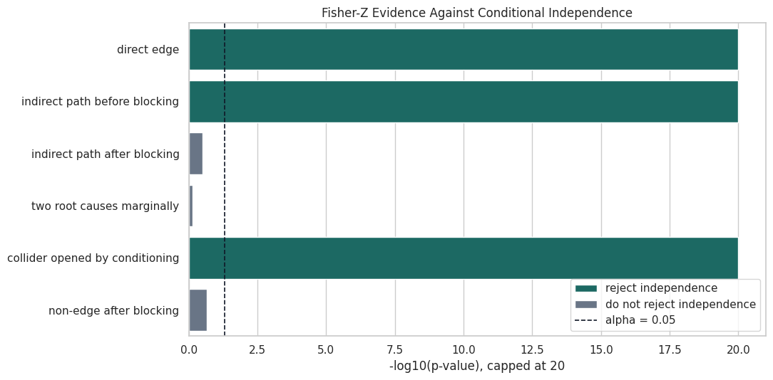
Visualize Fisher-Z Decisions

The next plot turns the previous p-values into capped -log10(p). Larger bars mean stronger evidence against independence. The dashed line marks the usual alpha level of 0.05. This visual form is useful because p-values can span many orders of magnitude; exact values remain in the table.

plot_df = fisherz_results.copy()
plot_df["minus_log10_p"] = capped_minus_log10(plot_df["p_value"])
alpha_line = -np.log10(ALPHA)

fig, ax = plt.subplots(figsize=(11, 5.5))
sns.barplot(
    data=plot_df,
    x="minus_log10_p",
    y="case",
    hue="decision_at_0_05",
    dodge=False,
    palette={"reject independence": "#0f766e", "do not reject independence": "#64748b"},
    ax=ax,
)
ax.axvline(alpha_line, color="#111827", linestyle="--", linewidth=1.2, label="alpha = 0.05")
ax.set_title("Fisher-Z Evidence Against Conditional Independence")
ax.set_xlabel("-log10(p-value), capped at 20")
ax.set_ylabel("")
ax.set_xlim(0, PLOT_LOG_CAP + 1)
ax.legend(loc="lower right")
plt.tight_layout()
fisherz_bar_path = FIGURE_DIR / f"{NOTEBOOK_PREFIX}_fisherz_case_decisions.png"
fig.savefig(fisherz_bar_path, dpi=160, bbox_inches="tight")
plt.show()

The visual split is clean: direct or opened paths have very large evidence against independence, while blocked paths and independent roots stay below the decision line. This is the local testing behavior PC-style algorithms depend on.

Conditioning-Set Size And Path Blocking

A conditioning set can block a path, open a collider, or add noise to the test. The next table follows one pair, need and renewal, as we add conditioning variables. This pair starts associated because there are directed and backdoor-style paths through the graph.

conditioning_progression = [
    (),
    ("intent",),
    ("match",),
    ("engagement",),
    ("intent", "match"),
    ("intent", "engagement"),
    ("match", "engagement"),
    ("intent", "match", "engagement"),
]

conditioning_rows = []
for conditioning_set in conditioning_progression:
    p_value = linear_runner("need", "renewal", conditioning_set)
    conditioning_rows.append(
        {
            "x": "need",
            "y": "renewal",
            "conditioning_set": ", ".join(conditioning_set) or "none",
            "conditioning_set_size": len(conditioning_set),
            "p_value": p_value,
            "p_value_display": p_value_label(p_value),
            "decision_at_0_05": decision_from_p_value(p_value),
        }
    )

conditioning_path_table = pd.DataFrame(conditioning_rows)
conditioning_path_table.to_csv(TABLE_DIR / f"{NOTEBOOK_PREFIX}_conditioning_set_progression.csv", index=False)
conditioning_path_table

	x	y	conditioning_set	conditioning_set_size	p_value	p_value_display	decision_at_0_05
0	need	renewal	none	0	0.000000	<1e-300	reject independence
1	need	renewal	intent	1	0.000000	<1e-300	reject independence
2	need	renewal	match	1	0.000000	<1e-300	reject independence
3	need	renewal	engagement	1	0.000000	<1e-300	reject independence
4	need	renewal	intent, match	2	0.185264	0.185	do not reject independence
5	need	renewal	intent, engagement	2	0.134290	0.134	do not reject independence
6	need	renewal	match, engagement	2	0.000000	<1e-300	reject independence
7	need	renewal	intent, match, engagement	3	0.308830	0.309	do not reject independence

The p-value changes as we block more of the relevant paths. The final conditioning set includes intent, match, and engagement, which blocks the main ways need and renewal are connected in the base graph.

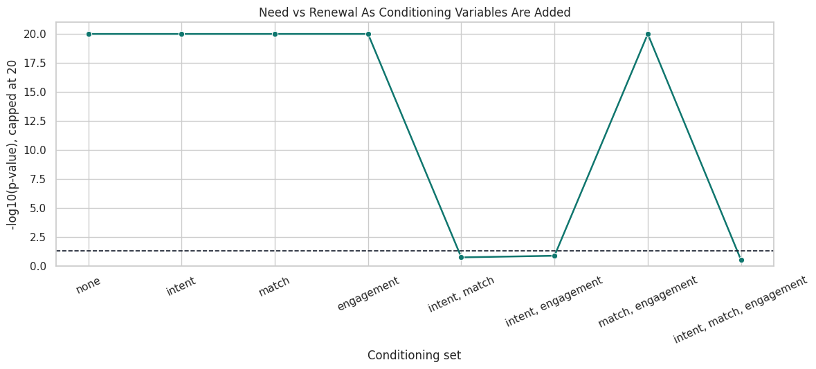
Plot The Conditioning Progression

This plot shows the same progression in decision-space. It reinforces a practical point: conditioning is not just “adding controls.” In graphical terms, each variable can block or open a path depending on where it sits in the DAG.

progression_plot = conditioning_path_table.copy()
progression_plot["minus_log10_p"] = capped_minus_log10(progression_plot["p_value"])

fig, ax = plt.subplots(figsize=(12, 5.5))
sns.lineplot(
    data=progression_plot,
    x="conditioning_set",
    y="minus_log10_p",
    marker="o",
    linewidth=1.8,
    color="#0f766e",
    ax=ax,
)
ax.axhline(-np.log10(ALPHA), color="#111827", linestyle="--", linewidth=1.2)
ax.set_title("Need vs Renewal As Conditioning Variables Are Added")
ax.set_xlabel("Conditioning set")
ax.set_ylabel("-log10(p-value), capped at 20")
ax.set_ylim(0, PLOT_LOG_CAP + 1)
ax.tick_params(axis="x", rotation=25)
plt.tight_layout()
conditioning_plot_path = FIGURE_DIR / f"{NOTEBOOK_PREFIX}_conditioning_set_progression.png"
fig.savefig(conditioning_plot_path, dpi=160, bbox_inches="tight")
plt.show()

The line drops below the alpha threshold only when the conditioning set blocks enough of the graph. This is why PC searches over many conditioning sets instead of relying on marginal associations.

Alpha Sensitivity

The alpha threshold controls how easily a test rejects independence. A larger alpha keeps more edges because it rejects independence more often. A smaller alpha removes edges more aggressively. The next cell shows decisions for the same Fisher-Z cases under several alpha values.

alpha_values = [0.001, 0.01, 0.05, 0.10]
alpha_rows = []
for _, row in fisherz_results.iterrows():
    for alpha in alpha_values:
        alpha_rows.append(
            {
                "case": row["case"],
                "p_value": row["p_value"],
                "alpha": alpha,
                "decision": decision_from_p_value(row["p_value"], alpha=alpha),
            }
        )

alpha_sensitivity = pd.DataFrame(alpha_rows)
alpha_sensitivity.to_csv(TABLE_DIR / f"{NOTEBOOK_PREFIX}_alpha_sensitivity_decisions.csv", index=False)
alpha_sensitivity.pivot(index="case", columns="alpha", values="decision")

alpha	0.001	0.010	0.050	0.100
case
collider opened by conditioning	reject independence	reject independence	reject independence	reject independence
direct edge	reject independence	reject independence	reject independence	reject independence
indirect path after blocking	do not reject independence	do not reject independence	do not reject independence	do not reject independence
indirect path before blocking	reject independence	reject independence	reject independence	reject independence
non-edge after blocking	do not reject independence	do not reject independence	do not reject independence	do not reject independence
two root causes marginally	do not reject independence	do not reject independence	do not reject independence	do not reject independence

Most clear cases are stable across alpha values, but borderline cases can flip. This is why later graph notebooks will include alpha sensitivity instead of reporting one graph as if the threshold were ordained.

Sample Size Sensitivity

Conditional independence tests need enough data. Small samples can fail to detect real dependence or can produce unstable p-values. This cell repeats three Fisher-Z checks across several sample sizes.

sample_cases = [
    {
        "case": "direct edge need-match",
        "x": "need",
        "y": "match",
        "conditioning_set": (),
    },
    {
        "case": "blocked non-edge need-renewal",
        "x": "need",
        "y": "renewal",
        "conditioning_set": ("intent", "match", "engagement"),
    },
    {
        "case": "opened collider need-intent",
        "x": "need",
        "y": "intent",
        "conditioning_set": ("match",),
    },
]

sample_sizes = [100, 250, 500, 1_000, 2_500]
sample_rows = []
linear_data = datasets["linear_gaussian"]
for sample_size in sample_sizes:
    sample_df = linear_data.sample(n=sample_size, random_state=RANDOM_SEED + sample_size)
    sample_runner = make_ci_runner(sample_df, base_nodes, "fisherz")
    for case in sample_cases:
        p_value = sample_runner(case["x"], case["y"], case["conditioning_set"])
        sample_rows.append(
            {
                "sample_size": sample_size,
                "case": case["case"],
                "conditioning_set": ", ".join(case["conditioning_set"]) or "none",
                "p_value": p_value,
                "decision_at_0_05": decision_from_p_value(p_value),
            }
        )

sample_size_sensitivity = pd.DataFrame(sample_rows)
sample_size_sensitivity.to_csv(TABLE_DIR / f"{NOTEBOOK_PREFIX}_sample_size_sensitivity.csv", index=False)
sample_size_sensitivity

	sample_size	case	conditioning_set	p_value	decision_at_0_05
0	100	direct edge need-match	none	3.498170e-07	reject independence
1	100	blocked non-edge need-renewal	intent, match, engagement	2.673226e-01	do not reject independence
2	100	opened collider need-intent	match	0.000000e+00	reject independence
3	250	direct edge need-match	none	0.000000e+00	reject independence
4	250	blocked non-edge need-renewal	intent, match, engagement	1.185747e-01	do not reject independence
5	250	opened collider need-intent	match	0.000000e+00	reject independence
6	500	direct edge need-match	none	0.000000e+00	reject independence
7	500	blocked non-edge need-renewal	intent, match, engagement	8.016450e-01	do not reject independence
8	500	opened collider need-intent	match	0.000000e+00	reject independence
9	1000	direct edge need-match	none	0.000000e+00	reject independence
10	1000	blocked non-edge need-renewal	intent, match, engagement	5.320839e-01	do not reject independence
11	1000	opened collider need-intent	match	0.000000e+00	reject independence
12	2500	direct edge need-match	none	0.000000e+00	reject independence
13	2500	blocked non-edge need-renewal	intent, match, engagement	3.088303e-01	do not reject independence
14	2500	opened collider need-intent	match	0.000000e+00	reject independence

The strongest dependence patterns are usually detected even with smaller samples. The blocked case is more variable because the expected result is “do not reject independence,” which is always harder to prove from finite data.

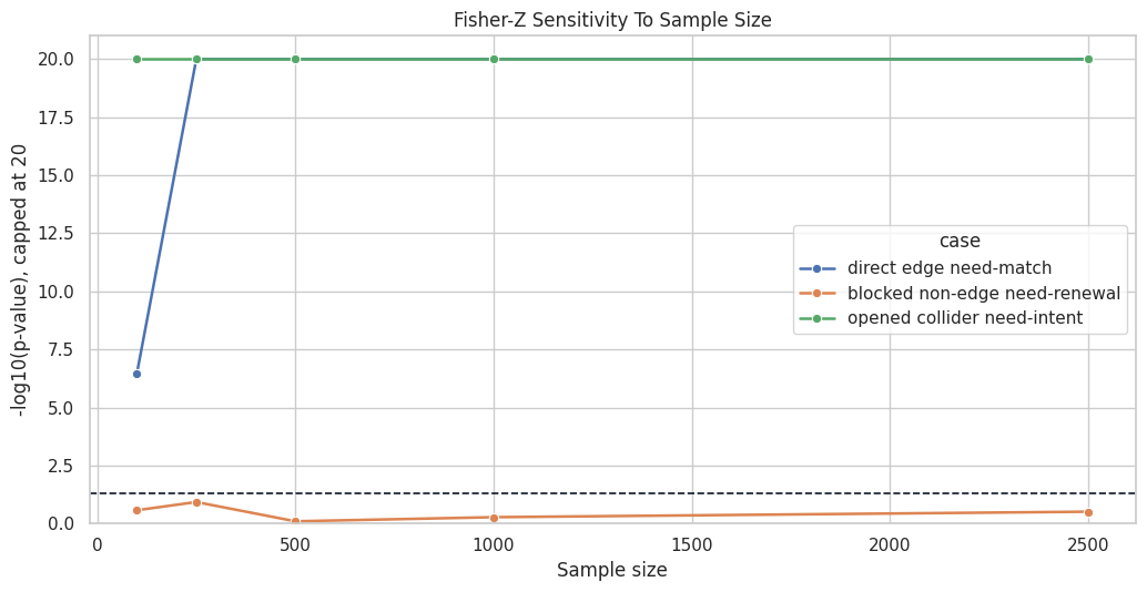
Plot Sample Size Sensitivity

The next plot shows how evidence against independence changes with sample size. The y-axis again uses capped -log10(p) so small p-values are visible without letting underflow dominate the scale.

sample_plot = sample_size_sensitivity.copy()
sample_plot["minus_log10_p"] = capped_minus_log10(sample_plot["p_value"])

fig, ax = plt.subplots(figsize=(10.5, 5.5))
sns.lineplot(
    data=sample_plot,
    x="sample_size",
    y="minus_log10_p",
    hue="case",
    marker="o",
    linewidth=1.8,
    ax=ax,
)
ax.axhline(-np.log10(ALPHA), color="#111827", linestyle="--", linewidth=1.2)
ax.set_title("Fisher-Z Sensitivity To Sample Size")
ax.set_xlabel("Sample size")
ax.set_ylabel("-log10(p-value), capped at 20")
ax.set_ylim(0, PLOT_LOG_CAP + 1)
plt.tight_layout()
sample_size_plot_path = FIGURE_DIR / f"{NOTEBOOK_PREFIX}_sample_size_sensitivity.png"
fig.savefig(sample_size_plot_path, dpi=160, bbox_inches="tight")
plt.show()

The plot makes the practical lesson visible: p-values are not only about graph structure; they also reflect sample size. A discovery graph learned from 100 rows can differ from one learned from 2,500 rows even if the data-generating DAG is identical.

Marginal P-Value Matrix

Before running a full algorithm, it is useful to inspect all pairwise marginal tests. This matrix is not a graph, but it reveals which variable pairs are strongly associated before conditioning.

def marginal_p_value_matrix(dataframe, columns, method):
    runner = make_ci_runner(dataframe, columns, method)
    matrix = pd.DataFrame(np.ones((len(columns), len(columns))), index=columns, columns=columns)
    for i, x in enumerate(columns):
        for j, y in enumerate(columns):
            if i >= j:
                continue
            p_value = runner(x, y, ())
            matrix.loc[x, y] = p_value
            matrix.loc[y, x] = p_value
    return matrix

fisherz_marginal_p = marginal_p_value_matrix(datasets["linear_gaussian"], base_nodes, "fisherz")
fisherz_marginal_p.to_csv(TABLE_DIR / f"{NOTEBOOK_PREFIX}_fisherz_marginal_p_matrix.csv")
fisherz_marginal_p

	need	intent	match	engagement	renewal	support
need	1.000000	0.742852	0.0	0.0	0.0	0.0
intent	0.742852	1.000000	0.0	0.0	0.0	0.0
match	0.000000	0.000000	1.0	0.0	0.0	0.0
engagement	0.000000	0.000000	0.0	1.0	0.0	0.0
renewal	0.000000	0.000000	0.0	0.0	1.0	0.0
support	0.000000	0.000000	0.0	0.0	0.0	1.0

Many non-adjacent pairs have very small marginal p-values because they are connected through paths in the DAG. This is the reason causal discovery cannot stop at pairwise testing.

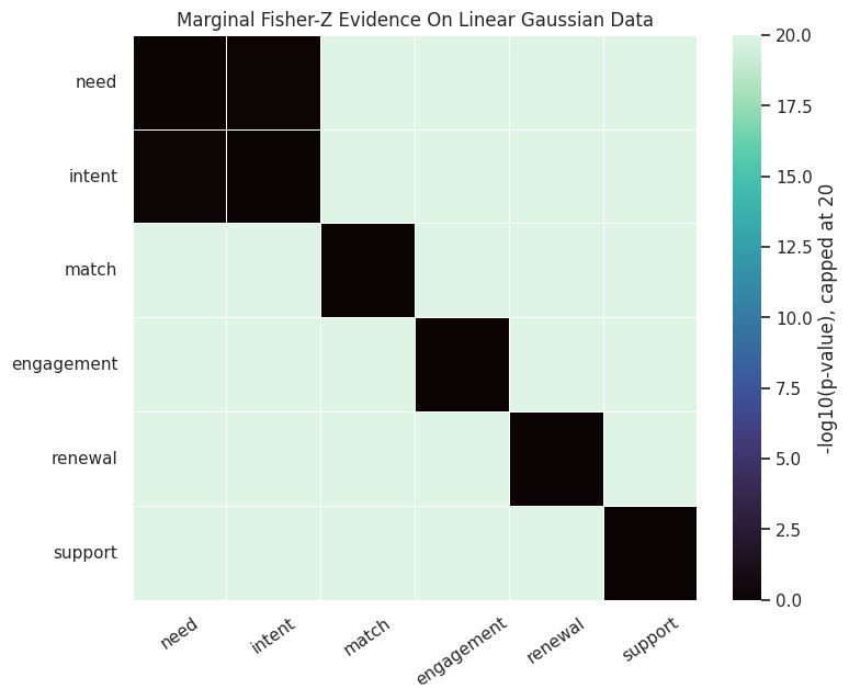
Heatmap Of Marginal Evidence

The heatmap shows the same p-value matrix as capped -log10(p). Bright cells are strong pairwise associations. The diagonal is set to zero because a variable is not tested against itself.

heatmap_values = fisherz_marginal_p.apply(lambda column: capped_minus_log10(column)).copy()
heatmap_array = heatmap_values.to_numpy(copy=True)
np.fill_diagonal(heatmap_array, 0)
heatmap_values = pd.DataFrame(heatmap_array, index=heatmap_values.index, columns=heatmap_values.columns)

fig, ax = plt.subplots(figsize=(8, 6.5))
sns.heatmap(
    heatmap_values,
    cmap="mako",
    linewidths=0.5,
    square=True,
    cbar_kws={"label": "-log10(p-value), capped at 20"},
    ax=ax,
)
ax.set_title("Marginal Fisher-Z Evidence On Linear Gaussian Data")
ax.tick_params(axis="x", rotation=35)
ax.tick_params(axis="y", rotation=0)
plt.tight_layout()
marginal_heatmap_path = FIGURE_DIR / f"{NOTEBOOK_PREFIX}_fisherz_marginal_p_heatmap.png"
fig.savefig(marginal_heatmap_path, dpi=160, bbox_inches="tight")
plt.show()

The heatmap is dense because marginal dependence travels along causal paths. PC-style algorithms become useful because they search for conditioning sets that explain away indirect associations.

Nonlinear Dependence: Fisher-Z vs KCI

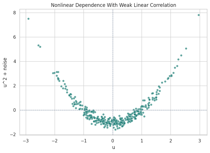
Fisher-Z is based on partial correlation, so it is naturally tuned to linear dependence. Kernel conditional independence tests can detect broader nonlinear relationships, but they are more expensive. The next demo creates a deliberately simple nonlinear pair: v = u^2 + noise. The correlation can be close to zero even though the variables are dependent.

nonlinear_rng = np.random.default_rng(RANDOM_SEED + 200)
nonlinear_demo = pd.DataFrame({"u": nonlinear_rng.normal(size=350)})
nonlinear_demo["v"] = (nonlinear_demo["u"] ** 2 - 1) + nonlinear_rng.normal(scale=0.25, size=len(nonlinear_demo))

nonlinear_demo_corr = nonlinear_demo["u"].corr(nonlinear_demo["v"])
fisherz_pair_runner = make_ci_runner(nonlinear_demo, ["u", "v"], "fisherz")
kci_pair_runner = make_ci_runner(nonlinear_demo, ["u", "v"], "kci")

nonlinear_test_comparison = pd.DataFrame(
    [
        {
            "test": "fisherz",
            "relationship": "u with u^2 + noise",
            "pearson_correlation": nonlinear_demo_corr,
            "p_value": fisherz_pair_runner("u", "v", ()),
        },
        {
            "test": "kci",
            "relationship": "u with u^2 + noise",
            "pearson_correlation": nonlinear_demo_corr,
            "p_value": kci_pair_runner("u", "v", ()),
        },
    ]
)
nonlinear_test_comparison["p_value_display"] = nonlinear_test_comparison["p_value"].map(p_value_label)
nonlinear_test_comparison["decision_at_0_05"] = nonlinear_test_comparison["p_value"].map(decision_from_p_value)
nonlinear_test_comparison.to_csv(TABLE_DIR / f"{NOTEBOOK_PREFIX}_nonlinear_fisherz_vs_kci.csv", index=False)
nonlinear_test_comparison

	test	relationship	pearson_correlation	p_value	p_value_display	decision_at_0_05
0	fisherz	u with u^2 + noise	0.021327	0.691117	0.691	do not reject independence
1	kci	u with u^2 + noise	0.021327	0.000000	<1e-300	reject independence

The Fisher-Z p-value does not reject independence because the linear correlation is weak. KCI rejects independence because the nonlinear relationship is real. This is the cleanest reminder that test choice encodes assumptions.

Visualize The Nonlinear Pair

The scatterplot makes the previous table obvious. A straight-line correlation test is looking for the wrong shape, while a nonlinear test can detect the curved relationship.

fig, ax = plt.subplots(figsize=(7.5, 5.5))
sns.scatterplot(data=nonlinear_demo, x="u", y="v", s=28, alpha=0.65, color="#0f766e", ax=ax)
ax.axhline(0, color="#94a3b8", linewidth=1, linestyle="--")
ax.axvline(0, color="#94a3b8", linewidth=1, linestyle="--")
ax.set_title("Nonlinear Dependence With Weak Linear Correlation")
ax.set_xlabel("u")
ax.set_ylabel("u^2 + noise")
plt.tight_layout()
nonlinear_pair_path = FIGURE_DIR / f"{NOTEBOOK_PREFIX}_nonlinear_pair_demo.png"
fig.savefig(nonlinear_pair_path, dpi=160, bbox_inches="tight")
plt.show()

The curved pattern is visually clear. A future nonlinear-discovery notebook can use this same lesson at graph scale: if the relationship is nonlinear, a linear test may produce misleading local decisions.

KCI On The Nonlinear Synthetic Dataset

Now we use KCI on a subset of the nonlinear continuous dataset from notebook 02. KCI is more expensive than Fisher-Z, so this example samples a few hundred rows and tests only a small number of relationships.

nonlinear_sample = datasets["nonlinear_continuous"].sample(n=350, random_state=RANDOM_SEED)
nonlinear_kci_runner = make_ci_runner(nonlinear_sample, base_nodes, "kci")
nonlinear_fisherz_runner = make_ci_runner(nonlinear_sample, base_nodes, "fisherz")

nonlinear_cases = [
    {"case": "true edge need-match", "x": "need", "y": "match", "conditioning_set": ()},
    {"case": "true edge match-engagement", "x": "match", "y": "engagement", "conditioning_set": ()},
    {"case": "blocked need-renewal", "x": "need", "y": "renewal", "conditioning_set": ("intent", "match", "engagement")},
]

nonlinear_ci_rows = []
for case in nonlinear_cases:
    for method_name, runner in [("fisherz", nonlinear_fisherz_runner), ("kci", nonlinear_kci_runner)]:
        p_value = runner(case["x"], case["y"], case["conditioning_set"])
        nonlinear_ci_rows.append(
            {
                "case": case["case"],
                "test": method_name,
                "conditioning_set": ", ".join(case["conditioning_set"]) or "none",
                "p_value": p_value,
                "p_value_display": p_value_label(p_value),
                "decision_at_0_05": decision_from_p_value(p_value),
            }
        )

nonlinear_dataset_test_comparison = pd.DataFrame(nonlinear_ci_rows)
nonlinear_dataset_test_comparison.to_csv(TABLE_DIR / f"{NOTEBOOK_PREFIX}_nonlinear_dataset_test_comparison.csv", index=False)
nonlinear_dataset_test_comparison

	case	test	conditioning_set	p_value	p_value_display	decision_at_0_05
0	true edge need-match	fisherz	none	0.000000	<1e-300	reject independence
1	true edge need-match	kci	none	0.000000	<1e-300	reject independence
2	true edge match-engagement	fisherz	none	0.000000	<1e-300	reject independence
3	true edge match-engagement	kci	none	0.000000	<1e-300	reject independence
4	blocked need-renewal	fisherz	intent, match, engagement	0.221437	0.221	do not reject independence
5	blocked need-renewal	kci	intent, match, engagement	0.193640	0.194	do not reject independence

The nonlinear dataset is less tidy than the two-variable demo, but the same caution applies. KCI can detect nonlinear dependence, while Fisher-Z is faster and simpler when its assumptions are reasonable.

Discrete Data: Chi-Square And G-Square

For discrete variables, causal-learn provides chi-square and G-square conditional independence tests. We use the discrete_mixed dataset from notebook 02. The cases mirror the Fisher-Z section, but the method now matches categorical data.

discrete_columns = base_nodes
discrete_chisq_runner = make_ci_runner(datasets["discrete_mixed"], discrete_columns, "chisq")
discrete_gsq_runner = make_ci_runner(datasets["discrete_mixed"], discrete_columns, "gsq")

discrete_cases = [
    {
        "case": "direct edge",
        "x": "need",
        "y": "match",
        "conditioning_set": (),
        "expected_pattern": "dependent because need affects match probability",
    },
    {
        "case": "indirect path before blocking",
        "x": "need",
        "y": "renewal",
        "conditioning_set": (),
        "expected_pattern": "dependent through downstream paths",
    },
    {
        "case": "indirect path after blocking",
        "x": "need",
        "y": "renewal",
        "conditioning_set": ("intent", "match", "engagement"),
        "expected_pattern": "weaker after blocking observed paths",
    },
    {
        "case": "blocked non-edge",
        "x": "need",
        "y": "support",
        "conditioning_set": ("intent", "match", "engagement"),
        "expected_pattern": "approximately independent after blocking paths through engagement",
    },
]

discrete_rows = []
for case in discrete_cases:
    for method_name, runner in [("chisq", discrete_chisq_runner), ("gsq", discrete_gsq_runner)]:
        p_value = runner(case["x"], case["y"], case["conditioning_set"])
        discrete_rows.append(
            {
                **case,
                "test": method_name,
                "conditioning_set": ", ".join(case["conditioning_set"]) or "none",
                "p_value": p_value,
                "p_value_display": p_value_label(p_value),
                "decision_at_0_05": decision_from_p_value(p_value),
            }
        )

discrete_test_results = pd.DataFrame(discrete_rows)
discrete_test_results.to_csv(TABLE_DIR / f"{NOTEBOOK_PREFIX}_discrete_chisq_gsq_results.csv", index=False)
discrete_test_results

	case	x	y	conditioning_set	expected_pattern	test	p_value	p_value_display	decision_at_0_05
0	direct edge	need	match	none	dependent because need affects match probability	chisq	1.807196e-40	1.81e-40	reject independence
1	direct edge	need	match	none	dependent because need affects match probability	gsq	4.869422e-41	4.87e-41	reject independence
2	indirect path before blocking	need	renewal	none	dependent through downstream paths	chisq	1.784279e-06	1.78e-06	reject independence
3	indirect path before blocking	need	renewal	none	dependent through downstream paths	gsq	1.749210e-06	1.75e-06	reject independence
4	indirect path after blocking	need	renewal	intent, match, engagement	weaker after blocking observed paths	chisq	1.751088e-01	0.175	do not reject independence
5	indirect path after blocking	need	renewal	intent, match, engagement	weaker after blocking observed paths	gsq	1.736190e-01	0.174	do not reject independence
6	blocked non-edge	need	support	intent, match, engagement	approximately independent after blocking paths through engagement	chisq	4.495724e-01	0.450	do not reject independence
7	blocked non-edge	need	support	intent, match, engagement	approximately independent after blocking paths through engagement	gsq	4.407588e-01	0.441	do not reject independence

Chi-square and G-square tell the same broad story here. Direct and unblocked paths show dependence, while blocked non-edges are less likely to reject independence. In sparse categorical problems, these two tests can differ more, so both are worth understanding.

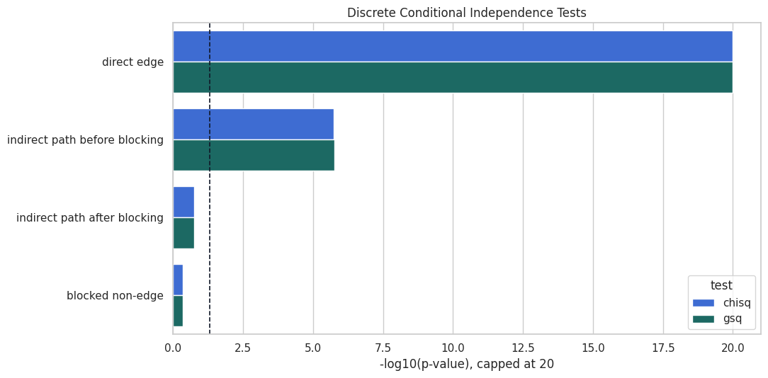
Discrete Test Decisions Side By Side

This plot compares chi-square and G-square p-values for the discrete cases. It is useful to see whether the two tests agree before using either one inside a full graph search.

discrete_plot = discrete_test_results.copy()
discrete_plot["minus_log10_p"] = capped_minus_log10(discrete_plot["p_value"])

fig, ax = plt.subplots(figsize=(11, 5.5))
sns.barplot(
    data=discrete_plot,
    x="minus_log10_p",
    y="case",
    hue="test",
    palette={"chisq": "#2563eb", "gsq": "#0f766e"},
    ax=ax,
)
ax.axvline(-np.log10(ALPHA), color="#111827", linestyle="--", linewidth=1.2)
ax.set_title("Discrete Conditional Independence Tests")
ax.set_xlabel("-log10(p-value), capped at 20")
ax.set_ylabel("")
ax.set_xlim(0, PLOT_LOG_CAP + 1)
plt.tight_layout()
discrete_plot_path = FIGURE_DIR / f"{NOTEBOOK_PREFIX}_discrete_chisq_gsq_comparison.png"
fig.savefig(discrete_plot_path, dpi=160, bbox_inches="tight")
plt.show()

The paired bars are close, which is reassuring for this synthetic dataset. The bigger lesson is that the discrete tests are designed for count data, while Fisher-Z is designed for continuous partial correlations.

Missing Values And mv_fisherz

Real datasets often have missing values. This section creates controlled missingness in the linear Gaussian data and compares two approaches:

• complete-case Fisher-Z, which drops rows with missing values in the variables involved in the test;
• causal-learn’s mv_fisherz, which is designed for missing-value settings.

This is a teaching example, not a universal missing-data solution. Missingness mechanisms still need their own causal thinking.

missing_rng = np.random.default_rng(RANDOM_SEED + 300)
missing_data = datasets["linear_gaussian"].copy()
missing_probability = 0.08
missing_mask = missing_rng.random(missing_data.shape) < missing_probability
missing_data = missing_data.mask(missing_mask)

missing_summary = pd.DataFrame(
    {
        "variable": missing_data.columns,
        "missing_rate": missing_data.isna().mean().values,
        "observed_count": missing_data.notna().sum().values,
    }
)
missing_summary.to_csv(TABLE_DIR / f"{NOTEBOOK_PREFIX}_missing_value_summary.csv", index=False)
missing_summary

	variable	missing_rate	observed_count
0	need	0.0756	2311
1	intent	0.0804	2299
2	match	0.0892	2277
3	engagement	0.0796	2301
4	renewal	0.0732	2317
5	support	0.0868	2283

The missing rates are close to the designed 8 percent level. Because the missingness was injected randomly here, it is much simpler than the missingness patterns we would worry about in real data.

Compare Complete-Case Fisher-Z And Missing-Value Fisher-Z

The next cell runs the same cases under complete-case Fisher-Z and mv_fisherz. For complete-case testing, each row must be observed for the pair and conditioning variables in that specific test.

def complete_case_fisherz(dataframe, x, y, conditioning_set=()):
    """Run Fisher-Z after dropping rows missing any variable needed for this test."""
    required_columns = [x, y, *conditioning_set]
    complete = dataframe[required_columns].dropna()
    runner = make_ci_runner(complete, required_columns, "fisherz")
    return runner(x, y, conditioning_set), len(complete)

mv_runner = make_ci_runner(missing_data, base_nodes, "mv_fisherz")
missing_cases = [
    {"case": "direct edge need-match", "x": "need", "y": "match", "conditioning_set": ()},
    {"case": "blocked need-renewal", "x": "need", "y": "renewal", "conditioning_set": ("intent", "match", "engagement")},
    {"case": "opened collider need-intent", "x": "need", "y": "intent", "conditioning_set": ("match",)},
]

missing_test_rows = []
for case in missing_cases:
    cc_p_value, cc_rows = complete_case_fisherz(missing_data, case["x"], case["y"], case["conditioning_set"])
    mv_p_value = mv_runner(case["x"], case["y"], case["conditioning_set"])
    missing_test_rows.extend(
        [
            {
                "case": case["case"],
                "approach": "complete_case_fisherz",
                "rows_used": cc_rows,
                "conditioning_set": ", ".join(case["conditioning_set"]) or "none",
                "p_value": cc_p_value,
                "p_value_display": p_value_label(cc_p_value),
                "decision_at_0_05": decision_from_p_value(cc_p_value),
            },
            {
                "case": case["case"],
                "approach": "mv_fisherz",
                "rows_used": len(missing_data),
                "conditioning_set": ", ".join(case["conditioning_set"]) or "none",
                "p_value": mv_p_value,
                "p_value_display": p_value_label(mv_p_value),
                "decision_at_0_05": decision_from_p_value(mv_p_value),
            },
        ]
    )

missing_test_comparison = pd.DataFrame(missing_test_rows)
missing_test_comparison.to_csv(TABLE_DIR / f"{NOTEBOOK_PREFIX}_missing_value_fisherz_comparison.csv", index=False)
missing_test_comparison

	case	approach	rows_used	conditioning_set	p_value	p_value_display	decision_at_0_05
0	direct edge need-match	complete_case_fisherz	2101	none	0.000000	<1e-300	reject independence
1	direct edge need-match	mv_fisherz	2500	none	0.000000	<1e-300	reject independence
2	blocked need-renewal	complete_case_fisherz	1659	intent, match, engagement	0.113165	0.113	do not reject independence
3	blocked need-renewal	mv_fisherz	2500	intent, match, engagement	0.113165	0.113	do not reject independence
4	opened collider need-intent	complete_case_fisherz	1940	match	0.000000	<1e-300	reject independence
5	opened collider need-intent	mv_fisherz	2500	match	0.000000	<1e-300	reject independence

The two approaches agree on the broad teaching patterns here. The complete-case row count drops most when the conditioning set is larger, which is one reason missingness can become more damaging in high-dimensional discovery.

Conditioning Set Size And Data Requirements

The number of possible conditioning sets grows quickly with the number of variables. Even before running PC, we can count how many candidate sets exist at each size for a pair of variables. This shows why constraint-based discovery can become expensive as graphs grow.

from math import comb

n_variables = len(base_nodes)
conditioning_count_rows = []
for conditioning_size in range(n_variables - 1):
    available_variables = n_variables - 2
    count_for_one_pair = comb(available_variables, conditioning_size) if conditioning_size <= available_variables else 0
    conditioning_count_rows.append(
        {
            "conditioning_set_size": conditioning_size,
            "candidate_sets_for_one_pair": count_for_one_pair,
            "why_it_matters": "More sets mean more tests and more chances for finite-sample instability.",
        }
    )

conditioning_set_counts = pd.DataFrame(conditioning_count_rows)
conditioning_set_counts.to_csv(TABLE_DIR / f"{NOTEBOOK_PREFIX}_conditioning_set_counts.csv", index=False)
conditioning_set_counts

	conditioning_set_size	candidate_sets_for_one_pair	why_it_matters
0	0	1	More sets mean more tests and more chances for finite-sample instability.
1	1	4	More sets mean more tests and more chances for finite-sample instability.
2	2	6	More sets mean more tests and more chances for finite-sample instability.
3	3	4	More sets mean more tests and more chances for finite-sample instability.
4	4	1	More sets mean more tests and more chances for finite-sample instability.

With six variables this is still tiny. With dozens or hundreds of variables, the search space becomes a real computational and statistical problem. This is why practical discovery workflows often use prior knowledge, variable screening, or stability checks.

What To Report With Independence Tests

This final guide summarizes what should be reported when conditional independence tests support a causal discovery graph. It is not enough to say “we ran PC.” A useful report should name the test, data type, alpha level, conditioning strategy, and sensitivity checks.

reporting_guide = pd.DataFrame(
    [
        {
            "report_item": "Test family",
            "example": "Fisher-Z for continuous linear Gaussian-style data",
            "why_it_matters": "The test defines what kind of independence claim is being evaluated.",
        },
        {
            "report_item": "Data type match",
            "example": "Chi-square or G-square for discrete variables",
            "why_it_matters": "A mismatched test can produce misleading graph edits.",
        },
        {
            "report_item": "Alpha threshold",
            "example": "alpha = 0.01, 0.05, and 0.10 sensitivity",
            "why_it_matters": "Graph structure can change when the rejection threshold changes.",
        },
        {
            "report_item": "Conditioning-set limits",
            "example": "Maximum conditioning size used by the algorithm",
            "why_it_matters": "Larger sets require more data and more tests.",
        },
        {
            "report_item": "Missing-data handling",
            "example": "Complete-case Fisher-Z versus mv_fisherz",
            "why_it_matters": "Missingness can change sample size and induce bias.",
        },
        {
            "report_item": "Nonlinear robustness",
            "example": "KCI check on suspected nonlinear relationships",
            "why_it_matters": "Linear tests can miss nonlinear dependence.",
        },
    ]
)

reporting_guide.to_csv(TABLE_DIR / f"{NOTEBOOK_PREFIX}_ci_reporting_guide.csv", index=False)
reporting_guide

	report_item	example	why_it_matters
0	Test family	Fisher-Z for continuous linear Gaussian-style data	The test defines what kind of independence claim is being evaluated.
1	Data type match	Chi-square or G-square for discrete variables	A mismatched test can produce misleading graph edits.
2	Alpha threshold	alpha = 0.01, 0.05, and 0.10 sensitivity	Graph structure can change when the rejection threshold changes.
3	Conditioning-set limits	Maximum conditioning size used by the algorithm	Larger sets require more data and more tests.
4	Missing-data handling	Complete-case Fisher-Z versus mv_fisherz	Missingness can change sample size and induce bias.
5	Nonlinear robustness	KCI check on suspected nonlinear relationships	Linear tests can miss nonlinear dependence.

This guide turns the technical test calls into a reporting checklist. A graph is easier to trust when the independence-test assumptions and sensitivity checks are visible.

Generated Artifact Manifest

The last cell lists the files created by this notebook. Later notebooks can reuse these tables and figures when explaining why a particular discovery algorithm behaved the way it did.

artifact_paths = sorted(list(TABLE_DIR.glob(f"{NOTEBOOK_PREFIX}_*")) + list(FIGURE_DIR.glob(f"{NOTEBOOK_PREFIX}_*")))
artifact_manifest = pd.DataFrame(
    [
        {
            "artifact_type": "figure" if path.parent == FIGURE_DIR else "table",
            "path": str(path.relative_to(NOTEBOOK_DIR)),
            "size_kb": round(path.stat().st_size / 1024, 1),
        }
        for path in artifact_paths
    ]
)
artifact_manifest.to_csv(TABLE_DIR / f"{NOTEBOOK_PREFIX}_artifact_manifest.csv", index=False)
artifact_manifest

	artifact_type	path	size_kb
0	figure	outputs/figures/03_conditioning_set_progression.png	136.6
1	figure	outputs/figures/03_discrete_chisq_gsq_comparison.png	61.8
2	figure	outputs/figures/03_fisherz_case_decisions.png	87.3
3	figure	outputs/figures/03_fisherz_marginal_p_heatmap.png	77.7
4	figure	outputs/figures/03_nonlinear_pair_demo.png	85.5
5	figure	outputs/figures/03_sample_size_sensitivity.png	82.2
6	table	outputs/tables/03_alpha_sensitivity_decisions.csv	1.6
7	table	outputs/tables/03_artifact_manifest.csv	1.2
8	table	outputs/tables/03_base_true_edges_used.csv	0.4
9	table	outputs/tables/03_ci_reporting_guide.csv	0.7
10	table	outputs/tables/03_ci_test_selection_guide.csv	1.1
11	table	outputs/tables/03_conditioning_set_counts.csv	0.4
12	table	outputs/tables/03_conditioning_set_progression.csv	0.6
13	table	outputs/tables/03_discrete_chisq_gsq_results.csv	1.3
14	table	outputs/tables/03_fisherz_linear_gaussian_cases.csv	1.0
15	table	outputs/tables/03_fisherz_marginal_p_matrix.csv	0.3
16	table	outputs/tables/03_loaded_dataset_summary.csv	0.3
17	table	outputs/tables/03_missing_value_fisherz_comparison.csv	0.7
18	table	outputs/tables/03_missing_value_summary.csv	0.2
19	table	outputs/tables/03_nonlinear_dataset_test_comparison.csv	0.5
20	table	outputs/tables/03_nonlinear_fisherz_vs_kci.csv	0.2
21	table	outputs/tables/03_sample_size_sensitivity.csv	1.2

The independence-test layer is now ready. The next notebook can run the PC algorithm on continuous data and use these ideas to explain why edges are removed, why some directions remain unresolved, and why alpha sensitivity matters.