causal-learn Tutorial 01: Graphs, DAGs, CPDAGs, PAGs, And Evaluation

This notebook builds the graph vocabulary that the rest of the causal-learn tutorial will rely on. Before running PC, FCI, GES, LiNGAM, or time-series discovery, we need to understand what those algorithms return. A causal discovery result is not just a picture: it is a compact statement about adjacencies, edge directions, ambiguous directions, possible hidden confounding, and what the observed data can or cannot distinguish.

The central question here is: when an algorithm returns a graph, how should we read it, compare it to a known answer, and report it responsibly? We will use small teaching graphs so every edge can be inspected by hand. The same ideas scale to larger graphs where manual inspection is impossible.

By the end, you should be comfortable with four recurring ideas:

A DAG is a fully directed acyclic graph: it says which variables are direct causes of which other variables under the assumed variable set.
A CPDAG represents a Markov equivalence class of DAGs: some directions are compelled, while other edges remain reversible from observational data alone.
A PAG is used when latent confounders or selection effects may exist: circles and bidirected edges communicate uncertainty and hidden-variable risk.
Evaluation metrics such as adjacency precision, adjacency recall, arrow precision, arrow recall, and SHD answer different questions; no single score fully summarizes graph quality.

Notebook Flow

We will move from concepts to code in small steps:

Set up imports, output folders, and package-version checks.
Build a tiny true DAG using causal-learn graph objects.
Render the same graph in a clean teaching style.
Convert a simple DAG to a CPDAG and inspect why directions can disappear.
Compare DAGs, CPDAG-like outputs, and PAG-like outputs using endpoint marks.
Build graph-recovery metrics from first principles.
Cross-check one example with causal-learn’s built-in graph-comparison utilities.

The goal is not to memorize every internal graph method. The goal is to learn what each graph is claiming and how to translate that claim into evidence a reviewer can understand.

Setup

This first code cell prepares the notebook environment. It creates output directories for figures and tables, imports the graph classes we will use from causal-learn, and prints package versions so the notebook is reproducible. The figure-rendering code uses Graphviz through pydot because graph layout matters in a tutorial: if the graph is hard to read, the concept becomes harder than it needs to be.

from pathlib import Path
from importlib.metadata import PackageNotFoundError, version
import os
import warnings

# Keep matplotlib cache files inside the project instead of writing to a user-level cache.
os.environ.setdefault("MPLCONFIGDIR", str(Path.cwd() / ".matplotlib_cache"))

import numpy as np
import pandas as pd
import matplotlib.pyplot as plt
import seaborn as sns
import pydot
from IPython.display import Image, display

from causallearn.graph.GraphNode import GraphNode
from causallearn.graph.Dag import Dag
from causallearn.graph.GeneralGraph import GeneralGraph
from causallearn.graph.Edge import Edge
from causallearn.graph.Endpoint import Endpoint
from causallearn.utils.DAG2CPDAG import dag2cpdag
from causallearn.graph.SHD import SHD
from causallearn.graph.AdjacencyConfusion import AdjacencyConfusion
from causallearn.graph.ArrowConfusion import ArrowConfusion

warnings.filterwarnings("ignore", category=FutureWarning)
sns.set_theme(style="whitegrid", context="notebook")
pd.set_option("display.max_columns", 80)
pd.set_option("display.max_colwidth", 120)

NOTEBOOK_DIR = Path.cwd()
if NOTEBOOK_DIR.name != "causal_learn":
    NOTEBOOK_DIR = Path("notebooks/tutorials/causal_learn").resolve()
else:
    NOTEBOOK_DIR = NOTEBOOK_DIR.resolve()

OUTPUT_DIR = NOTEBOOK_DIR / "outputs"
FIGURE_DIR = OUTPUT_DIR / "figures"
TABLE_DIR = OUTPUT_DIR / "tables"
for directory in [OUTPUT_DIR, FIGURE_DIR, TABLE_DIR]:
    directory.mkdir(parents=True, exist_ok=True)

NOTEBOOK_PREFIX = "01"


def pkg_version(package_name: str) -> str:
    """Return a package version string without failing the notebook if metadata is unavailable."""
    try:
        return version(package_name)
    except PackageNotFoundError:
        return "not installed"

version_table = pd.DataFrame(
    [
        {"package": "causal-learn", "version": pkg_version("causal-learn")},
        {"package": "pandas", "version": pkg_version("pandas")},
        {"package": "numpy", "version": pkg_version("numpy")},
        {"package": "matplotlib", "version": pkg_version("matplotlib")},
        {"package": "seaborn", "version": pkg_version("seaborn")},
        {"package": "pydot", "version": pkg_version("pydot")},
    ]
)
version_table

	package	version
0	causal-learn	0.1.4.5
1	pandas	3.0.2
2	numpy	2.4.4
3	matplotlib	3.10.9
4	seaborn	0.13.2
5	pydot	4.0.1

The version table is a small but useful reproducibility check. Discovery algorithms are sensitive to implementation details, and graph classes can change across library versions. Keeping the versions visible makes it easier to explain later why a result may differ from another machine or tutorial.

Graph Concept Map

This table gives the minimum vocabulary needed before touching algorithms. A common mistake is to treat every returned graph as if it were a fully oriented causal DAG. That is too strong for many discovery methods. PC often returns a CPDAG-like object because observational data cannot always orient every edge. FCI returns a PAG-like object because it explicitly allows hidden confounding. Score-based methods such as GES also work over equivalence classes rather than simply selecting one arbitrary DAG.

Read this table as a translation layer between algorithm output and plain English.

graph_concepts = pd.DataFrame(
    [
        {
            "concept": "DAG",
            "stands_for": "Directed acyclic graph",
            "edge_example": "A -> B",
            "plain_language": "A is represented as a direct cause of B, and cycles are not allowed.",
            "why_it_matters": "This is the cleanest causal story, but observational discovery often cannot justify every direction.",
        },
        {
            "concept": "Skeleton",
            "stands_for": "Adjacency pattern without directions",
            "edge_example": "A - B",
            "plain_language": "A and B are connected somehow, but the direction is ignored.",
            "why_it_matters": "Skeleton quality asks whether the algorithm found the right variable pairs before asking whether directions are right.",
        },
        {
            "concept": "CPDAG",
            "stands_for": "Completed partially directed acyclic graph",
            "edge_example": "A -> B and B - C",
            "plain_language": "Directed edges are compelled across an equivalence class; undirected edges are reversible.",
            "why_it_matters": "It prevents overclaiming directions that the observed conditional independences cannot identify.",
        },
        {
            "concept": "PAG",
            "stands_for": "Partial ancestral graph",
            "edge_example": "A o-> B or A <-> B",
            "plain_language": "Endpoint marks encode uncertainty and possible hidden confounding.",
            "why_it_matters": "It is the right language when unmeasured common causes may be present.",
        },
        {
            "concept": "SHD",
            "stands_for": "Structural Hamming Distance",
            "edge_example": "count of edits",
            "plain_language": "How many edge additions, deletions, or orientation changes are needed to move from one graph to another.",
            "why_it_matters": "It is compact, but it hides which kind of error occurred unless paired with precision/recall metrics.",
        },
    ]
)

graph_concepts.to_csv(TABLE_DIR / f"{NOTEBOOK_PREFIX}_graph_concept_map.csv", index=False)
graph_concepts

	concept	stands_for	edge_example	plain_language	why_it_matters
0	DAG	Directed acyclic graph	A -> B	A is represented as a direct cause of B, and cycles are not allowed.	This is the cleanest causal story, but observational discovery often cannot justify every direction.
1	Skeleton	Adjacency pattern without directions	A - B	A and B are connected somehow, but the direction is ignored.	Skeleton quality asks whether the algorithm found the right variable pairs before asking whether directions are right.
2	CPDAG	Completed partially directed acyclic graph	A -> B and B - C	Directed edges are compelled across an equivalence class; undirected edges are reversible.	It prevents overclaiming directions that the observed conditional independences cannot identify.
3	PAG	Partial ancestral graph	A o-> B or A <-> B	Endpoint marks encode uncertainty and possible hidden confounding.	It is the right language when unmeasured common causes may be present.
4	SHD	Structural Hamming Distance	count of edits	How many edge additions, deletions, or orientation changes are needed to move from one graph to another.	It is compact, but it hides which kind of error occurred unless paired with precision/recall metrics.

This table sets up the main reporting habit for causal discovery: separate whether two variables are connected from whether the direction is known. A graph can have an excellent skeleton and still be weak on directions. That is not necessarily a failure; sometimes the data genuinely do not contain enough information to orient an edge.

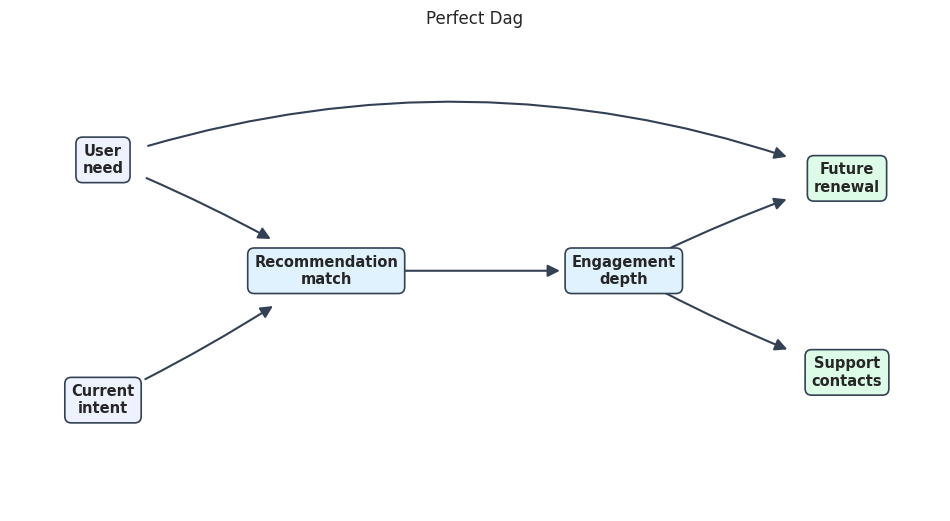
A Small Teaching DAG

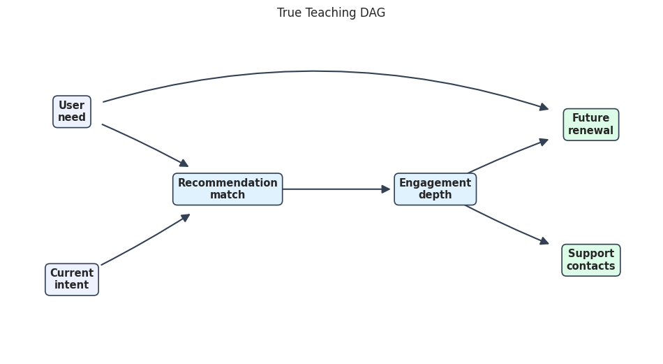
Now we create a small true graph. The variables are intentionally generic and product-analytics flavored, but the graph is artificial so we can know the answer. We will use it as a controlled reference for the rest of the notebook.

The story is:

Need and Intent jointly influence whether a user sees a good Match.
Match drives Engagement.
Engagement affects both Renewal and Support demand.
Need also directly affects Renewal, so not all renewal differences are explained by engagement.

This is a DAG because every edge has one direction and there is no directed cycle.

node_labels = {
    "Need": "User\nneed",
    "Intent": "Current\nintent",
    "Match": "Recommendation\nmatch",
    "Engagement": "Engagement\ndepth",
    "Renewal": "Future\nrenewal",
    "Support": "Support\ncontacts",
}

true_edge_table = pd.DataFrame(
    [
        {"source": "Need", "target": "Match", "mark": "-->", "reason": "Need affects what match quality means for the user."},
        {"source": "Intent", "target": "Match", "mark": "-->", "reason": "Current intent affects which recommendation feels relevant."},
        {"source": "Match", "target": "Engagement", "mark": "-->", "reason": "Better matching increases downstream engagement."},
        {"source": "Engagement", "target": "Renewal", "mark": "-->", "reason": "Deeper engagement can raise future value."},
        {"source": "Engagement", "target": "Support", "mark": "-->", "reason": "More engagement can create more opportunities for support contact."},
        {"source": "Need", "target": "Renewal", "mark": "-->", "reason": "Underlying need can directly affect renewal even after engagement."},
    ]
)

true_edge_table.to_csv(TABLE_DIR / f"{NOTEBOOK_PREFIX}_true_dag_edges.csv", index=False)
true_edge_table

	source	target	mark	reason
0	Need	Match	-->	Need affects what match quality means for the user.
1	Intent	Match	-->	Current intent affects which recommendation feels relevant.
2	Match	Engagement	-->	Better matching increases downstream engagement.
3	Engagement	Renewal	-->	Deeper engagement can raise future value.
4	Engagement	Support	-->	More engagement can create more opportunities for support contact.
5	Need	Renewal	-->	Underlying need can directly affect renewal even after engagement.

The edge table is deliberately explicit. In larger projects, keeping an edge table next to the graph helps reviewers understand whether an arrow came from domain assumptions, from an algorithm, or from a simulation design. Here it is our ground-truth answer key.

Building The DAG With causal-learn Objects

The previous cell was a plain pandas table. This cell builds the same graph using causal-learn’s graph classes. The important pieces are:

GraphNode: wraps the variable name.
Dag: stores a directed acyclic graph.
Edge: stores two endpoint marks.
Endpoint.TAIL and Endpoint.ARROW: together represent a directed edge from source to target.

In causal-learn notation, A --> B means the endpoint at A is a tail and the endpoint at B is an arrowhead.

def build_causallearn_graph(node_names, edge_table, graph_class=GeneralGraph):
    """Build a causal-learn graph from a table with source, target, and mark columns."""
    nodes = [GraphNode(name) for name in node_names]
    node_map = {node.get_name(): node for node in nodes}
    graph = graph_class(nodes)

    endpoint_map = {
        "-->": (Endpoint.TAIL, Endpoint.ARROW),
        "<--": (Endpoint.ARROW, Endpoint.TAIL),
        "---": (Endpoint.TAIL, Endpoint.TAIL),
        "<->": (Endpoint.ARROW, Endpoint.ARROW),
        "o->": (Endpoint.CIRCLE, Endpoint.ARROW),
        "<-o": (Endpoint.ARROW, Endpoint.CIRCLE),
        "o-o": (Endpoint.CIRCLE, Endpoint.CIRCLE),
    }

    for row in edge_table.itertuples(index=False):
        end1, end2 = endpoint_map[row.mark]
        graph.add_edge(Edge(node_map[row.source], node_map[row.target], end1, end2))

    return graph, node_map

node_order = list(node_labels)
true_dag, true_node_map = build_causallearn_graph(node_order, true_edge_table, graph_class=Dag)

causal_learn_edges = pd.DataFrame(
    {
        "causal_learn_edge_string": [str(edge) for edge in true_dag.get_graph_edges()]
    }
)
causal_learn_edges

	causal_learn_edge_string
0	Need --> Match
1	Need --> Renewal
2	Intent --> Match
3	Match --> Engagement
4	Engagement --> Renewal
5	Engagement --> Support

The causal-learn edge strings match the edge table: every edge is directed. This is the object form that algorithms and built-in graph metrics expect. The table form is still useful because it is easier to read, save, modify, and render in a teaching notebook.

Rendering The Teaching DAG

The next helper renders edge tables with Graphviz. The visual conventions are the same ones we will use throughout the tutorial:

--> is a directed edge.
--- is an undirected or reversible CPDAG edge.
<-> is a bidirected edge, often used to flag latent common-cause risk in mixed graphs.
o->, <-o, and o-o are PAG-style uncertain endpoints.

The fixed node positions are not part of the causal model. They simply make the picture easier to read and keep the notebook output stable across runs.

def render_edge_table_graph(
    edge_table,
    labels,
    positions,
    title,
    output_path,
    node_colors=None,
    edge_radii=None,
    circle_positions=None,
    edge_color="#334155",
    figsize=(12, 6),
):
    """Render an edge table using the shared tutorial DAG style."""
    node_colors = node_colors or {node: "#e0f2fe" for node in labels}
    edge_radii = edge_radii or {}
    circle_positions = circle_positions or {}

    fig, ax = plt.subplots(figsize=figsize)
    ax.set_xlim(0, 1)
    ax.set_ylim(0, 1)
    ax.set_axis_off()
    endpoint_circle_queue = []

    def endpoint_circle(source, target, near_source=True):
        """Queue a PAG circle endpoint, using explicit positions when provided."""
        side = "source" if near_source else "target"
        key = (source, target, side)
        if key in circle_positions:
            point = np.array(circle_positions[key], dtype=float)
        else:
            source_xy = np.array(positions[source], dtype=float)
            target_xy = np.array(positions[target], dtype=float)
            t = 0.18 if near_source else 0.82
            point = source_xy + t * (target_xy - source_xy)
        endpoint_circle_queue.append(point)

    for row in edge_table.itertuples(index=False):
        source = row.source
        target = row.target
        mark = row.mark
        rad = edge_radii.get((source, target), edge_radii.get((target, source), 0.0))
        linestyle = "-"
        arrowstyle = "-|>"
        xy = positions[target]
        xytext = positions[source]

        if mark == "<--":
            xy = positions[source]
            xytext = positions[target]
        elif mark == "---":
            arrowstyle = "-"
        elif mark == "<->":
            arrowstyle = "<|-|>"
        elif mark == "o->":
            endpoint_circle(source, target, near_source=True)
        elif mark == "<-o":
            xy = positions[source]
            xytext = positions[target]
            endpoint_circle(source, target, near_source=False)
        elif mark == "o-o":
            arrowstyle = "-"
            endpoint_circle(source, target, near_source=True)
            endpoint_circle(source, target, near_source=False)

        ax.annotate(
            "",
            xy=xy,
            xytext=xytext,
            arrowprops=dict(
                arrowstyle=arrowstyle,
                color=edge_color,
                linewidth=1.5,
                mutation_scale=18,
                shrinkA=34,
                shrinkB=46,
                linestyle=linestyle,
                connectionstyle=f"arc3,rad={rad}",
            ),
            zorder=1,
        )

    for point in endpoint_circle_queue:
        ax.scatter(
            point[0],
            point[1],
            s=34,
            facecolors="white",
            edgecolors=edge_color,
            linewidths=1.5,
            zorder=3,
        )

    for node, (x, y) in positions.items():
        ax.text(
            x,
            y,
            labels[node],
            ha="center",
            va="center",
            fontsize=10.5,
            fontweight="bold",
            bbox=dict(
                boxstyle="round,pad=0.45",
                facecolor=node_colors.get(node, "#e0f2fe"),
                edgecolor="#334155",
                linewidth=1.2,
            ),
            zorder=4,
        )

    ax.set_title(title, pad=18)
    output_path = Path(output_path)
    output_path.parent.mkdir(parents=True, exist_ok=True)
    fig.savefig(output_path, dpi=160, bbox_inches="tight")
    plt.show()
    return output_path

teaching_positions = {
    "Need": (0.10, 0.76),
    "Intent": (0.10, 0.24),
    "Match": (0.34, 0.52),
    "Engagement": (0.66, 0.52),
    "Renewal": (0.90, 0.72),
    "Support": (0.90, 0.30),
}

teaching_node_colors = {
    "Need": "#eef2ff",
    "Intent": "#eef2ff",
    "Match": "#e0f2fe",
    "Engagement": "#e0f2fe",
    "Renewal": "#dcfce7",
    "Support": "#dcfce7",
}

teaching_edge_radii = {
    ("Need", "Match"): -0.04,
    ("Intent", "Match"): 0.04,
    ("Match", "Engagement"): 0.00,
    ("Engagement", "Renewal"): -0.04,
    ("Engagement", "Support"): 0.04,
    ("Need", "Renewal"): -0.18,
    ("Intent", "Support"): 0.18,
}

true_dag_path = FIGURE_DIR / f"{NOTEBOOK_PREFIX}_true_teaching_dag.png"
render_edge_table_graph(
    true_edge_table,
    node_labels,
    teaching_positions,
    "True Teaching DAG",
    true_dag_path,
    node_colors=teaching_node_colors,
    edge_radii=teaching_edge_radii,
)

PosixPath('/home/apex/Documents/ranking_sys/notebooks/tutorials/causal_learn/outputs/figures/01_true_teaching_dag.png')

The rendered graph makes two structural features easy to see. First, Need and Intent form a collider at Match: Need -> Match <- Intent. Second, Renewal has two parents, Need and Engagement. These patterns matter because v-structures are often what allow observational discovery algorithms to orient some edges.

Endpoint Vocabulary

causal-learn graphs are built from endpoint marks, not just from whole-edge labels. This matters because algorithms such as FCI can return edges where one endpoint is known and the other is uncertain.

The whole-edge notation is a compact way to read the two endpoint marks together.

endpoint_vocabulary = pd.DataFrame(
    [
        {
            "whole_edge_mark": "A --> B",
            "endpoint_at_A": "TAIL",
            "endpoint_at_B": "ARROW",
            "typical_graph": "DAG, CPDAG, PAG",
            "meaning": "A is oriented as an ancestor/cause-side endpoint of B.",
        },
        {
            "whole_edge_mark": "A --- B",
            "endpoint_at_A": "TAIL",
            "endpoint_at_B": "TAIL",
            "typical_graph": "CPDAG",
            "meaning": "A and B are adjacent, but this edge is reversible within the equivalence class.",
        },
        {
            "whole_edge_mark": "A o-> B",
            "endpoint_at_A": "CIRCLE",
            "endpoint_at_B": "ARROW",
            "typical_graph": "PAG",
            "meaning": "The endpoint near A is uncertain; B has an arrowhead on this edge.",
        },
        {
            "whole_edge_mark": "A <-> B",
            "endpoint_at_A": "ARROW",
            "endpoint_at_B": "ARROW",
            "typical_graph": "PAG or mixed graph",
            "meaning": "Often read as possible latent common-cause structure between A and B.",
        },
        {
            "whole_edge_mark": "A o-o B",
            "endpoint_at_A": "CIRCLE",
            "endpoint_at_B": "CIRCLE",
            "typical_graph": "PAG",
            "meaning": "The relationship is adjacent, but both endpoint orientations remain unresolved.",
        },
    ]
)

endpoint_vocabulary.to_csv(TABLE_DIR / f"{NOTEBOOK_PREFIX}_endpoint_vocabulary.csv", index=False)
endpoint_vocabulary

	whole_edge_mark	endpoint_at_A	endpoint_at_B	typical_graph	meaning
0	A --> B	TAIL	ARROW	DAG, CPDAG, PAG	A is oriented as an ancestor/cause-side endpoint of B.
1	A --- B	TAIL	TAIL	CPDAG	A and B are adjacent, but this edge is reversible within the equivalence class.
2	A o-> B	CIRCLE	ARROW	PAG	The endpoint near A is uncertain; B has an arrowhead on this edge.
3	A <-> B	ARROW	ARROW	PAG or mixed graph	Often read as possible latent common-cause structure between A and B.
4	A o-o B	CIRCLE	CIRCLE	PAG	The relationship is adjacent, but both endpoint orientations remain unresolved.

This endpoint view is the cleanest way to avoid overclaiming. A circle is not decorative; it is a statement that the available information has not resolved that endpoint. When writing up a discovery result, those unresolved marks should be preserved rather than silently converted to arrows.

DAG To CPDAG: Why Some Directions Disappear

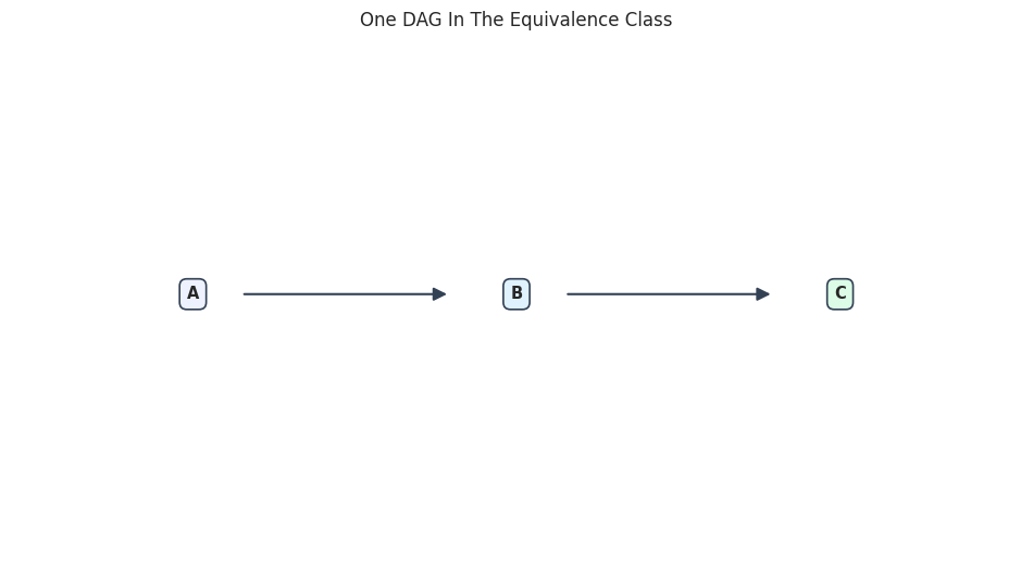
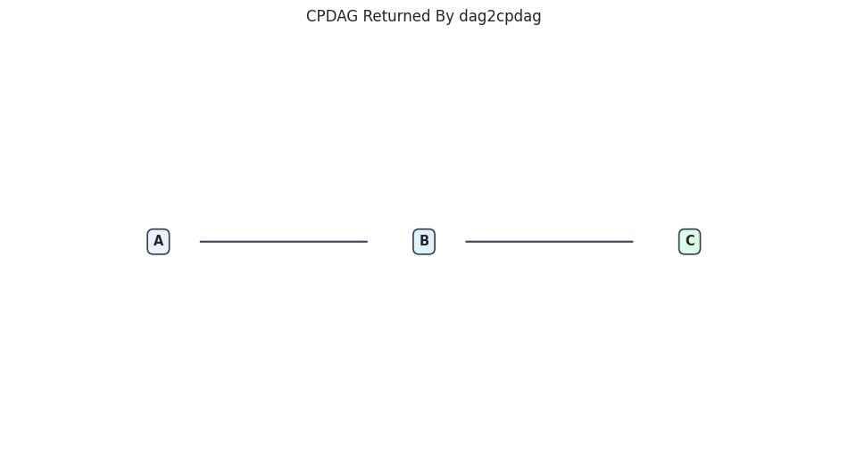
A CPDAG represents all DAGs that imply the same observational conditional independences. If several DAGs are Markov equivalent, observational data alone cannot choose among them without extra assumptions, interventions, time ordering, or background knowledge.

The classic example is a three-node chain. A -> B -> C and A <- B -> C share the same skeleton and have no unshielded collider, so they are Markov equivalent. In a CPDAG, the reversible edges become undirected.

chain_labels = {"A": "A", "B": "B", "C": "C"}
chain_positions = {"A": (0.18, 0.52), "B": (0.50, 0.52), "C": (0.82, 0.52)}
chain_node_colors = {"A": "#eef2ff", "B": "#e0f2fe", "C": "#dcfce7"}
chain_edges = pd.DataFrame(
    [
        {"source": "A", "target": "B", "mark": "-->", "reason": "First link in a simple chain."},
        {"source": "B", "target": "C", "mark": "-->", "reason": "Second link in a simple chain."},
    ]
)

chain_dag, _ = build_causallearn_graph(list(chain_labels), chain_edges, graph_class=Dag)
chain_cpdag = dag2cpdag(chain_dag)


def causallearn_edges_to_table(graph):
    """Convert causal-learn edges into a small readable endpoint table."""
    records = []
    for edge in graph.get_graph_edges():
        endpoint1 = str(edge.get_endpoint1())
        endpoint2 = str(edge.get_endpoint2())
        source = edge.get_node1().get_name()
        target = edge.get_node2().get_name()
        mark_lookup = {
            ("TAIL", "ARROW"): "-->",
            ("ARROW", "TAIL"): "<--",
            ("TAIL", "TAIL"): "---",
            ("ARROW", "ARROW"): "<->",
            ("CIRCLE", "ARROW"): "o->",
            ("ARROW", "CIRCLE"): "<-o",
            ("CIRCLE", "CIRCLE"): "o-o",
        }
        records.append(
            {
                "source": source,
                "target": target,
                "endpoint_at_source": endpoint1,
                "endpoint_at_target": endpoint2,
                "mark": mark_lookup.get((endpoint1, endpoint2), f"{endpoint1}/{endpoint2}"),
                "causal_learn_string": str(edge),
            }
        )
    return pd.DataFrame(records)

chain_cpdag_table = causallearn_edges_to_table(chain_cpdag)
chain_cpdag_table.to_csv(TABLE_DIR / f"{NOTEBOOK_PREFIX}_chain_cpdag_edges.csv", index=False)

chain_dag_path = FIGURE_DIR / f"{NOTEBOOK_PREFIX}_chain_dag.png"
chain_cpdag_path = FIGURE_DIR / f"{NOTEBOOK_PREFIX}_chain_cpdag.png"

render_edge_table_graph(chain_edges, chain_labels, chain_positions, "One DAG In The Equivalence Class", chain_dag_path, node_colors=chain_node_colors)
render_edge_table_graph(
    chain_cpdag_table.assign(reason="reversible edge in the CPDAG"),
    chain_labels,
    chain_positions,
    "CPDAG Returned By dag2cpdag",
    chain_cpdag_path,
    node_colors=chain_node_colors,
    edge_color="#334155",
)

chain_cpdag_table

	source	target	endpoint_at_source	endpoint_at_target	mark	causal_learn_string
0	A	B	TAIL	TAIL	---	A --- B
1	B	C	TAIL	TAIL	---	B --- C

The CPDAG table shows undirected --- edges. That does not mean there is no causal relationship. It means the equivalence class does not force a single direction for those adjacencies. This is one of the most important habits in causal discovery reporting: uncertainty about direction should stay visible.

Markov Equivalence And V-Structures

Two DAGs are Markov equivalent when they have the same skeleton and the same unshielded colliders, also called v-structures. The next cell compares three small graphs:

A chain: A -> B -> C.
A fork: A <- B -> C.
A collider: A -> B <- C.

The chain and fork have the same skeleton and no collider. The collider has the same skeleton but a different v-structure, so it implies different conditional independence behavior.

def skeleton_from_edges(edge_pairs):
    """Return undirected adjacencies as sorted frozensets."""
    return {frozenset([source, target]) for source, target in edge_pairs}


def v_structures_from_edges(edge_pairs):
    """Find unshielded colliders A -> B <- C in a directed edge list."""
    parents = {}
    all_edges = set(edge_pairs)
    for source, target in edge_pairs:
        parents.setdefault(target, set()).add(source)

    v_structures = []
    for child, parent_set in parents.items():
        sorted_parents = sorted(parent_set)
        for i, left_parent in enumerate(sorted_parents):
            for right_parent in sorted_parents[i + 1 :]:
                parents_adjacent = (
                    (left_parent, right_parent) in all_edges
                    or (right_parent, left_parent) in all_edges
                )
                if not parents_adjacent:
                    v_structures.append(f"{left_parent} -> {child} <- {right_parent}")
    return sorted(v_structures)

small_graphs = {
    "chain_A_to_B_to_C": [("A", "B"), ("B", "C")],
    "fork_B_to_A_and_C": [("B", "A"), ("B", "C")],
    "collider_A_and_C_to_B": [("A", "B"), ("C", "B")],
}

equivalence_rows = []
for graph_name, edges in small_graphs.items():
    equivalence_rows.append(
        {
            "graph": graph_name,
            "directed_edges": ", ".join([f"{a}->{b}" for a, b in edges]),
            "skeleton": ", ".join(sorted(["-".join(sorted(edge)) for edge in skeleton_from_edges(edges)])),
            "unshielded_colliders": "; ".join(v_structures_from_edges(edges)) or "none",
        }
    )

equivalence_table = pd.DataFrame(equivalence_rows)
equivalence_table.to_csv(TABLE_DIR / f"{NOTEBOOK_PREFIX}_markov_equivalence_examples.csv", index=False)
equivalence_table

	graph	directed_edges	skeleton	unshielded_colliders
0	chain_A_to_B_to_C	A->B, B->C	A-B, B-C	none
1	fork_B_to_A_and_C	B->A, B->C	A-B, B-C	none
2	collider_A_and_C_to_B	A->B, C->B	A-B, B-C	A -> B <- C

The chain and fork rows share the same skeleton and both list none for unshielded colliders. The collider row has the same adjacencies but a different collider pattern. This is why v-structures are so valuable: they are one of the few orientation patterns observational conditional independence tests can often identify.

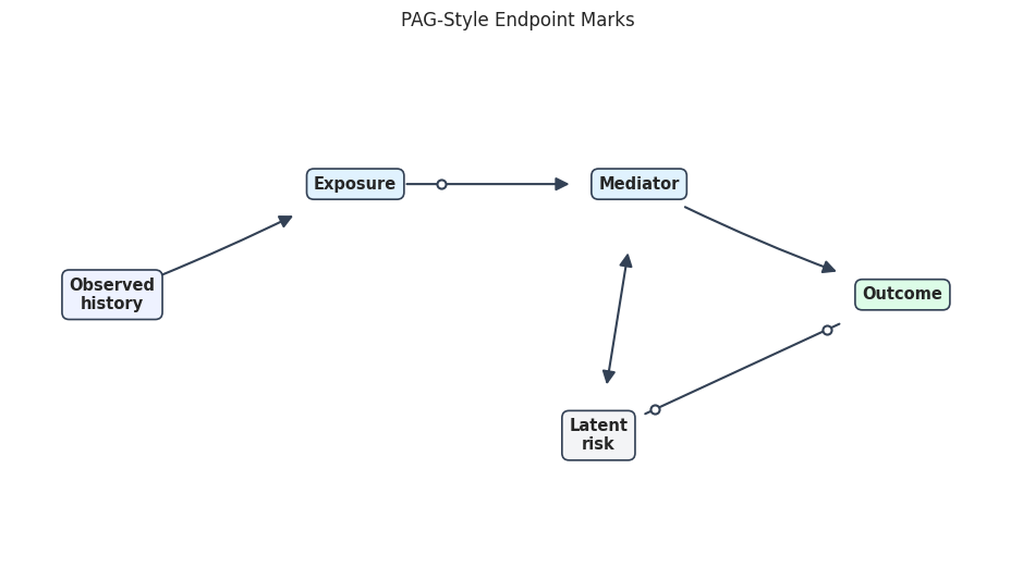
PAG-Style Edge Marks

A PAG is the graph language used by algorithms such as FCI when latent confounders or selection effects are allowed. In practice, this means the algorithm is less willing to pretend that every relevant cause has been measured.

The graph below is not the output of an algorithm. It is a hand-made teaching graph showing the edge marks you will later see in FCI-style notebooks.

pag_labels = {
    "X": "Observed\nhistory",
    "A": "Exposure",
    "M": "Mediator",
    "Y": "Outcome",
    "U": "Latent\nrisk",
}
pag_positions = {
    "X": (0.10, 0.52),
    "A": (0.34, 0.74),
    "M": (0.62, 0.74),
    "Y": (0.88, 0.52),
    "U": (0.58, 0.24),
}
pag_node_colors = {
    "X": "#eef2ff",
    "A": "#e0f2fe",
    "M": "#e0f2fe",
    "Y": "#dcfce7",
    "U": "#f3f4f6",
}
pag_edge_radii = {
    ("X", "A"): 0.03,
    ("A", "M"): 0.00,
    ("M", "Y"): 0.04,
    ("U", "M"): 0.00,
    ("U", "Y"): 0.00,
}
pag_circle_positions = {
    ("A", "M", "source"): (0.425, 0.74),
    ("U", "Y", "source"): (0.635, 0.292),
    ("U", "Y", "target"): (0.805, 0.450),
}
pag_edge_table = pd.DataFrame(
    [
        {"source": "X", "target": "A", "mark": "-->", "meaning": "Observed history is oriented into exposure."},
        {"source": "A", "target": "M", "mark": "o->", "meaning": "The mediator endpoint is an arrowhead; the exposure-side endpoint is unresolved."},
        {"source": "M", "target": "Y", "mark": "-->", "meaning": "Mediator is oriented into outcome."},
        {"source": "U", "target": "M", "mark": "<->", "meaning": "Bidirected edge flags hidden common-cause style risk."},
        {"source": "U", "target": "Y", "mark": "o-o", "meaning": "Both endpoint orientations remain unresolved for this illustrative relationship."},
    ]
)

pag_graph, _ = build_causallearn_graph(list(pag_labels), pag_edge_table, graph_class=GeneralGraph)
pag_strings = [str(edge) for edge in pag_graph.get_graph_edges()]

pag_path = FIGURE_DIR / f"{NOTEBOOK_PREFIX}_pag_edge_marks.png"
render_edge_table_graph(
    pag_edge_table,
    pag_labels,
    pag_positions,
    "PAG-Style Endpoint Marks",
    pag_path,
    node_colors=pag_node_colors,
    edge_radii=pag_edge_radii,
    circle_positions=pag_circle_positions,
    edge_color="#334155",
)

pag_edge_table.assign(causal_learn_string=pag_strings)

	source	target	mark	meaning	causal_learn_string
0	X	A	-->	Observed history is oriented into exposure.	X --> A
1	A	M	o->	The mediator endpoint is an arrowhead; the exposure-side endpoint is unresolved.	A o-> M
2	M	Y	-->	Mediator is oriented into outcome.	M --> Y
3	U	M	<->	Bidirected edge flags hidden common-cause style risk.	M <-> U
4	U	Y	o-o	Both endpoint orientations remain unresolved for this illustrative relationship.	Y o-o U

The key habit is to read each endpoint separately. For example, A o-> M is weaker than A -> M: it says there is an arrowhead at M, while the endpoint near A remains uncertain. This is exactly the sort of nuance that disappears if a PAG is redrawn as a simple DAG.

Graph Evaluation Metrics From First Principles

When a true graph is known, usually through simulation or a benchmark, we can evaluate learned graphs. It is useful to split evaluation into two layers:

Adjacency evaluation asks whether the right pairs of variables were connected, ignoring direction.
Direction evaluation asks whether the directed arrows match the true directions.

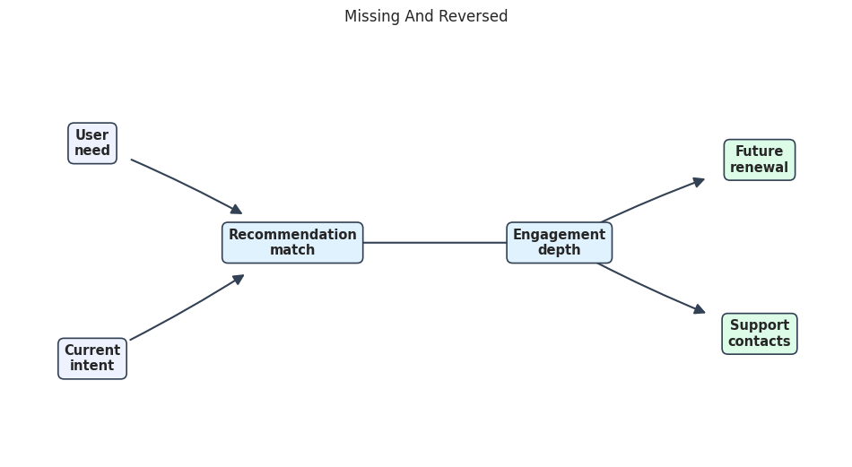
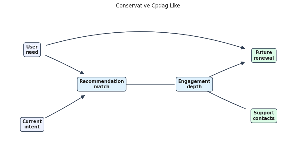
A conservative algorithm may recover the right adjacencies but leave many edges undirected. That should score well on skeleton recall but not necessarily on arrow recall. This distinction is more informative than one overall score.

def directed_edges_from_table(edge_table):
    """Extract directed claims from an edge table."""
    directed = set()
    for row in edge_table.itertuples(index=False):
        if row.mark == "-->":
            directed.add((row.source, row.target))
        elif row.mark == "<--":
            directed.add((row.target, row.source))
    return directed


def skeleton_from_table(edge_table):
    """Extract adjacency claims from an edge table, ignoring endpoint direction."""
    return {frozenset([row.source, row.target]) for row in edge_table.itertuples(index=False)}


def safe_ratio(numerator, denominator):
    return np.nan if denominator == 0 else numerator / denominator


def evaluate_edge_table(candidate_name, truth_table, estimated_table):
    """Compute readable skeleton and arrow metrics for one estimated graph."""
    truth_skeleton = skeleton_from_table(truth_table)
    estimated_skeleton = skeleton_from_table(estimated_table)
    truth_directed = directed_edges_from_table(truth_table)
    estimated_directed = directed_edges_from_table(estimated_table)

    skeleton_tp = len(truth_skeleton & estimated_skeleton)
    skeleton_fp = len(estimated_skeleton - truth_skeleton)
    skeleton_fn = len(truth_skeleton - estimated_skeleton)

    arrow_tp = len(truth_directed & estimated_directed)
    arrow_fp = len(estimated_directed - truth_directed)
    arrow_fn = len(truth_directed - estimated_directed)
    reversed_arrows = sum((target, source) in estimated_directed for source, target in truth_directed)

    skeleton_precision = safe_ratio(skeleton_tp, skeleton_tp + skeleton_fp)
    skeleton_recall = safe_ratio(skeleton_tp, skeleton_tp + skeleton_fn)
    arrow_precision = safe_ratio(arrow_tp, arrow_tp + arrow_fp)
    arrow_recall = safe_ratio(arrow_tp, arrow_tp + arrow_fn)

    return {
        "candidate": candidate_name,
        "skeleton_tp": skeleton_tp,
        "skeleton_fp": skeleton_fp,
        "skeleton_fn": skeleton_fn,
        "skeleton_precision": skeleton_precision,
        "skeleton_recall": skeleton_recall,
        "arrow_tp": arrow_tp,
        "arrow_fp": arrow_fp,
        "arrow_fn": arrow_fn,
        "arrow_precision": arrow_precision,
        "arrow_recall": arrow_recall,
        "reversed_arrows": reversed_arrows,
        "shd_like_edit_count": skeleton_fp + skeleton_fn + reversed_arrows,
    }

perfect_estimate = true_edge_table.copy()

extra_adjacency = pd.concat(
    [
        true_edge_table,
        pd.DataFrame(
            [{"source": "Intent", "target": "Support", "mark": "-->", "reason": "Spurious extra edge."}]
        ),
    ],
    ignore_index=True,
)

missing_and_reversed = pd.DataFrame(
    [
        {"source": "Need", "target": "Match", "mark": "-->", "reason": "Correct."},
        {"source": "Intent", "target": "Match", "mark": "-->", "reason": "Correct."},
        {"source": "Engagement", "target": "Match", "mark": "-->", "reason": "Reversed version of Match -> Engagement."},
        {"source": "Engagement", "target": "Renewal", "mark": "-->", "reason": "Correct."},
        {"source": "Engagement", "target": "Support", "mark": "-->", "reason": "Correct."},
    ]
)

conservative_cpdag_like = true_edge_table.copy()
conservative_cpdag_like.loc[
    conservative_cpdag_like["source"].eq("Match") & conservative_cpdag_like["target"].eq("Engagement"),
    "mark",
] = "---"
conservative_cpdag_like.loc[
    conservative_cpdag_like["source"].eq("Engagement") & conservative_cpdag_like["target"].eq("Support"),
    "mark",
] = "---"
conservative_cpdag_like["reason"] = "Same adjacency set, but two directions are intentionally left unresolved."

candidate_tables = {
    "perfect_dag": perfect_estimate,
    "extra_adjacency": extra_adjacency,
    "missing_and_reversed": missing_and_reversed,
    "conservative_cpdag_like": conservative_cpdag_like,
}

evaluation_table = pd.DataFrame(
    [evaluate_edge_table(name, true_edge_table, table) for name, table in candidate_tables.items()]
)

evaluation_table.to_csv(TABLE_DIR / f"{NOTEBOOK_PREFIX}_custom_graph_evaluation_metrics.csv", index=False)
evaluation_table

	candidate	skeleton_tp	skeleton_fp	skeleton_fn	skeleton_precision	skeleton_recall	arrow_tp	arrow_fp	arrow_fn	arrow_precision	arrow_recall	reversed_arrows	shd_like_edit_count
0	perfect_dag	6	0	0	1.000000	1.000000	6	0	0	1.000000	1.000000	0	0
1	extra_adjacency	6	1	0	0.857143	1.000000	6	1	0	0.857143	1.000000	0	1
2	missing_and_reversed	5	0	1	1.000000	0.833333	4	1	2	0.800000	0.666667	1	2
3	conservative_cpdag_like	6	0	0	1.000000	1.000000	4	0	2	1.000000	0.666667	0	0

The metric table shows why multiple scores are needed. The conservative CPDAG-like candidate has perfect skeleton precision and recall because it connects the right variable pairs, but its arrow recall is lower because it refuses to orient two edges. The missing-and-reversed candidate loses both an adjacency and a direction, which is a more serious structural error.

Visual Comparison Of Candidate Graphs

Tables are precise, but visual comparison helps diagnose the type of mistake. The next cell renders each candidate graph using the same node positions as the true DAG. Keeping the layout fixed makes differences easier to spot: an extra edge, a missing edge, a reversed edge, or an unresolved edge mark becomes visually obvious.

for candidate_name, candidate_table in candidate_tables.items():
    candidate_path = FIGURE_DIR / f"{NOTEBOOK_PREFIX}_{candidate_name}.png"
    render_edge_table_graph(
        candidate_table,
        node_labels,
        teaching_positions,
        candidate_name.replace("_", " ").title(),
        candidate_path,
        node_colors=teaching_node_colors,
        edge_radii=teaching_edge_radii,
        edge_color="#334155",
    )

The fixed-layout views make the reporting tradeoff tangible. A conservative graph may look less decisive, but it can be more honest. A graph with extra arrows may look impressive, yet it can encode false causal claims. In causal discovery, being explicit about uncertainty is usually better than making the graph look complete.

Cross-Checking With causal-learn Built-In Metrics

causal-learn includes graph-comparison utilities for common benchmark metrics. The next cell compares the true DAG to the missing_and_reversed candidate. We keep this as a cross-check instead of the only evaluation because built-in metric definitions can be compact and library-specific. For a report, it is useful to show both: the library score and a plain-language table that says what kind of mistake happened.

missing_reversed_graph, _ = build_causallearn_graph(node_order, missing_and_reversed, graph_class=GeneralGraph)

adj_confusion = AdjacencyConfusion(true_dag, missing_reversed_graph)
arrow_confusion = ArrowConfusion(true_dag, missing_reversed_graph)
shd_score = SHD(true_dag, missing_reversed_graph).get_shd()

causal_learn_metric_table = pd.DataFrame(
    [
        {"metric_family": "SHD", "metric": "structural_hamming_distance", "value": shd_score},
        {"metric_family": "Adjacency", "metric": "true_positive", "value": adj_confusion.get_adj_tp()},
        {"metric_family": "Adjacency", "metric": "false_positive", "value": adj_confusion.get_adj_fp()},
        {"metric_family": "Adjacency", "metric": "false_negative", "value": adj_confusion.get_adj_fn()},
        {"metric_family": "Adjacency", "metric": "precision", "value": adj_confusion.get_adj_precision()},
        {"metric_family": "Adjacency", "metric": "recall", "value": adj_confusion.get_adj_recall()},
        {"metric_family": "Arrow", "metric": "true_positive", "value": arrow_confusion.get_arrows_tp()},
        {"metric_family": "Arrow", "metric": "false_positive", "value": arrow_confusion.get_arrows_fp()},
        {"metric_family": "Arrow", "metric": "false_negative", "value": arrow_confusion.get_arrows_fn()},
        {"metric_family": "Arrow", "metric": "precision", "value": arrow_confusion.get_arrows_precision()},
        {"metric_family": "Arrow", "metric": "recall", "value": arrow_confusion.get_arrows_recall()},
    ]
)

causal_learn_metric_table.to_csv(TABLE_DIR / f"{NOTEBOOK_PREFIX}_causal_learn_builtin_metrics.csv", index=False)
causal_learn_metric_table

	metric_family	metric	value
0	SHD	structural_hamming_distance	2.000000
1	Adjacency	true_positive	5.000000
2	Adjacency	false_positive	0.000000
3	Adjacency	false_negative	1.000000
4	Adjacency	precision	1.000000
5	Adjacency	recall	0.833333
6	Arrow	true_positive	4.000000
7	Arrow	false_positive	1.000000
8	Arrow	false_negative	2.000000
9	Arrow	precision	0.800000
10	Arrow	recall	0.666667

The built-in metrics agree with the qualitative diagnosis: this candidate recovered most adjacencies but made direction mistakes. The important workflow lesson is to pair numeric metrics with an edge-level explanation. A single SHD value is useful for benchmarking, but it does not tell a stakeholder which causal claims changed.

Metric Selection Guide

This final guide summarizes which metric to emphasize for different discovery questions. The best metric depends on the decision the graph will support. If a graph will be used only to reduce a modeling feature set, adjacency recall may matter more than arrow precision. If a graph will support causal claims or intervention planning, arrow errors become much more consequential.

metric_selection_guide = pd.DataFrame(
    [
        {
            "question": "Did we find the right connected variable pairs?",
            "metric_to_start_with": "Adjacency precision and adjacency recall",
            "watch_out_for": "High adjacency recall can still hide many false directions.",
        },
        {
            "question": "Did we orient arrows correctly?",
            "metric_to_start_with": "Arrow precision and arrow recall",
            "watch_out_for": "A conservative CPDAG/PAG may leave valid uncertainty instead of making wrong arrow claims.",
        },
        {
            "question": "How far is the whole graph from the reference graph?",
            "metric_to_start_with": "SHD",
            "watch_out_for": "SHD is compact but should be decomposed into missing, extra, and reversed edge errors.",
        },
        {
            "question": "Can we use this graph for causal decisions?",
            "metric_to_start_with": "Edge-level audit plus domain review",
            "watch_out_for": "Graph recovery metrics do not validate causal assumptions by themselves.",
        },
    ]
)

metric_selection_guide.to_csv(TABLE_DIR / f"{NOTEBOOK_PREFIX}_metric_selection_guide.csv", index=False)
metric_selection_guide

	question	metric_to_start_with	watch_out_for
0	Did we find the right connected variable pairs?	Adjacency precision and adjacency recall	High adjacency recall can still hide many false directions.
1	Did we orient arrows correctly?	Arrow precision and arrow recall	A conservative CPDAG/PAG may leave valid uncertainty instead of making wrong arrow claims.
2	How far is the whole graph from the reference graph?	SHD	SHD is compact but should be decomposed into missing, extra, and reversed edge errors.
3	Can we use this graph for causal decisions?	Edge-level audit plus domain review	Graph recovery metrics do not validate causal assumptions by themselves.

This guide turns the notebook into a reusable checklist. Before reporting a discovered graph, decide whether the work needs adjacency recovery, direction recovery, equivalence-class reporting, or a decision-ready causal story. Different goals require different evidence.

Generated Artifacts

The last cell lists the files created by this notebook. Keeping outputs organized makes the tutorial easier to audit and makes it simple to reuse figures in a writeup or presentation.

generated_artifacts = pd.DataFrame(
    [
        {
            "artifact_type": "figure" if path.suffix.lower() in {".png", ".jpg", ".jpeg"} else "table",
            "path": str(path.relative_to(NOTEBOOK_DIR)),
            "size_kb": round(path.stat().st_size / 1024, 1),
        }
        for path in sorted(list(FIGURE_DIR.glob(f"{NOTEBOOK_PREFIX}_*")) + list(TABLE_DIR.glob(f"{NOTEBOOK_PREFIX}_*")))
    ]
)

generated_artifacts

	artifact_type	path	size_kb
0	figure	outputs/figures/01_chain_cpdag.png	21.7
1	figure	outputs/figures/01_chain_dag.png	20.9
2	figure	outputs/figures/01_conservative_cpdag_like.png	65.7
3	figure	outputs/figures/01_extra_adjacency.png	71.8
4	figure	outputs/figures/01_missing_and_reversed.png	58.2
5	figure	outputs/figures/01_pag_edge_marks.png	49.1
6	figure	outputs/figures/01_perfect_dag.png	62.8
7	figure	outputs/figures/01_true_teaching_dag.png	63.9
8	table	outputs/tables/01_causal_learn_builtin_metrics.csv	0.3
9	table	outputs/tables/01_chain_cpdag_edges.csv	0.1
10	table	outputs/tables/01_custom_graph_evaluation_metrics.csv	0.4
11	table	outputs/tables/01_endpoint_vocabulary.csv	0.6
12	table	outputs/tables/01_graph_concept_map.csv	1.2
13	table	outputs/tables/01_markov_equivalence_examples.csv	0.2
14	table	outputs/tables/01_metric_selection_guide.csv	0.6
15	table	outputs/tables/01_true_dag_edges.csv	0.5

The notebook now has the graph vocabulary needed for the rest of the causal-learn sequence. The next tutorial can start generating synthetic data because we now know exactly what the true graph means, how an algorithm might return a partially oriented version of it, and how to evaluate that output without flattening away uncertainty.