Advanced SEM and ML Mediation Models

The previous notebooks built the discovery-quality mediation design, estimated a transparent linear g-computation decomposition, and stress-tested the result across definitions and specifications. This notebook adds a more advanced modeling layer.

The goal is not to replace the earlier notebooks. The goal is to ask whether the same story survives when we use more flexible models and a more formal path-model framing.

This notebook has four advanced pieces:

• SEM-style path model: estimate the A -> M, M -> Y, and A -> Y paths as a formal mediation path decomposition.
• Cross-fitted ML nuisance models: estimate mediator and outcome nuisance functions with Linear Regression, LightGBM, and XGBoost without evaluating each row on models trained on that row.
• Heterogeneity analysis: check whether the discovery effect differs across prior activity, prior satisfaction, prior discovery, and user activity groups.
• Feature importance audit: inspect which covariates the tree-based nuisance models use most.

The main question remains the same: does high discovery exposure increase future user value, and is that effect meaningfully routed through same-day satisfaction depth?

1. Load Libraries and Paths

This cell imports the modeling libraries used in the notebook. LightGBM and XGBoost are used for flexible nuisance models, while linear models provide the transparent baseline and SEM-style path estimates. The path setup mirrors earlier notebooks so the outputs land in the same processed and writeup folders.

from pathlib import Path
import os
import warnings

os.environ.setdefault("OMP_NUM_THREADS", "1")
os.environ.setdefault("OPENBLAS_NUM_THREADS", "1")
os.environ.setdefault("MKL_NUM_THREADS", "1")
os.environ.setdefault("NUMEXPR_NUM_THREADS", "1")

import numpy as np
import pandas as pd
import seaborn as sns
import matplotlib.pyplot as plt
from IPython.display import display
from sklearn.base import clone
from sklearn.linear_model import LinearRegression
from sklearn.metrics import mean_absolute_error, mean_squared_error, r2_score
from sklearn.model_selection import GroupKFold
from sklearn.preprocessing import StandardScaler

from lightgbm import LGBMRegressor
from xgboost import XGBRegressor

warnings.filterwarnings("ignore", category=FutureWarning)

sns.set_theme(style="whitegrid", context="notebook")
plt.rcParams["figure.figsize"] = (11, 6)
plt.rcParams["axes.titlesize"] = 13
plt.rcParams["axes.labelsize"] = 11
pd.set_option("display.max_columns", 180)
pd.set_option("display.max_colwidth", 140)

PROJECT_ROOT = Path.cwd().resolve()
while not (PROJECT_ROOT / "data").exists() and PROJECT_ROOT.parent != PROJECT_ROOT:
    PROJECT_ROOT = PROJECT_ROOT.parent

PROCESSED_DIR = PROJECT_ROOT / "data" / "processed"
NOTEBOOK_DIR = PROJECT_ROOT / "notebooks" / "discovery_quality_mediation"
WRITEUP_DIR = NOTEBOOK_DIR / "writeup"
FIGURE_DIR = WRITEUP_DIR / "figures"
TABLE_DIR = WRITEUP_DIR / "tables"

FIGURE_DIR.mkdir(parents=True, exist_ok=True)
TABLE_DIR.mkdir(parents=True, exist_ok=True)

ANALYSIS_PANEL_INPUT = PROCESSED_DIR / "kuairec_discovery_quality_mediation_analysis_panel.parquet"
EFFECT_SUMMARY_INPUT = PROCESSED_DIR / "kuairec_discovery_quality_effect_summary.csv"
ROBUSTNESS_SUMMARY_INPUT = PROCESSED_DIR / "kuairec_discovery_quality_robustness_summary.csv"

SEM_PATH_OUTPUT = PROCESSED_DIR / "kuairec_discovery_quality_sem_path_results.csv"
SEM_BOOTSTRAP_OUTPUT = PROCESSED_DIR / "kuairec_discovery_quality_sem_bootstrap.csv"
ML_EFFECTS_OUTPUT = PROCESSED_DIR / "kuairec_discovery_quality_advanced_ml_effects.csv"
ML_PERFORMANCE_OUTPUT = PROCESSED_DIR / "kuairec_discovery_quality_advanced_ml_performance.csv"
HETEROGENEITY_OUTPUT = PROCESSED_DIR / "kuairec_discovery_quality_advanced_heterogeneity.csv"
FEATURE_IMPORTANCE_OUTPUT = PROCESSED_DIR / "kuairec_discovery_quality_advanced_feature_importance.csv"
ADVANCED_SUMMARY_OUTPUT = PROCESSED_DIR / "kuairec_discovery_quality_advanced_model_summary.csv"

The thread settings keep LightGBM and XGBoost from taking over the machine. The dataset is small enough that single-threaded tree models are still fast and easier to reproduce.

2. Load Analysis Inputs

This cell loads the saved mediation analysis panel and the previous result tables. The advanced notebook should not reconstruct the panel from raw logs; it should reuse the cleaned analysis object created earlier.

analysis_panel = pd.read_parquet(ANALYSIS_PANEL_INPUT)
effect_summary = pd.read_csv(EFFECT_SUMMARY_INPUT)
robustness_summary = pd.read_csv(ROBUSTNESS_SUMMARY_INPUT)

load_summary = pd.DataFrame(
    {
        "artifact": ["analysis_panel", "effect_summary", "robustness_summary"],
        "rows": [len(analysis_panel), len(effect_summary), len(robustness_summary)],
        "columns": [analysis_panel.shape[1], effect_summary.shape[1], robustness_summary.shape[1]],
    }
)

main_effects = effect_summary.query(
    "outcome == 'Y_future_interactions' and estimand in ['gcomp_total_effect', 'natural_direct_effect', 'natural_indirect_effect']"
)[["estimand", "estimate", "ci_95_lower", "ci_95_upper", "relative_effect"]]

display(load_summary)
display(main_effects.round(4))
display(robustness_summary.round(4))

	artifact	rows	columns
0	analysis_panel	8199	103
1	effect_summary	21	12
2	robustness_summary	4	9

	estimand	estimate	ci_95_lower	ci_95_upper	relative_effect
2	gcomp_total_effect	37.2781	32.2444	42.8135	0.1152
3	natural_direct_effect	38.5858	33.3634	43.7154	0.1192
4	natural_indirect_effect	-1.3077	-2.3047	-0.4290	-0.0036

	robustness_family	specifications	total_effect_min	total_effect_max	total_effect_share_positive	indirect_effect_min	indirect_effect_max	indirect_effect_share_positive	median_abs_indirect_to_total_ratio
0	threshold_sensitivity	4	37.2781	40.0555	1.0	-1.6532	-1.3077	0.0	0.0402
1	mediator_sensitivity	5	37.2560	37.3502	1.0	-1.7145	0.1281	0.2	0.0359
2	model_sensitivity	5	34.8085	37.6289	1.0	-1.5581	-0.9360	0.0	0.0351
3	outcome_sensitivity	1	37.2781	37.2781	1.0	-1.3077	-1.3077	0.0	0.0351

The earlier result is the benchmark. The advanced models should be judged against this reference, not treated as automatically better just because they are more flexible.

3. Define Variables and Control Sets

This cell defines the treatment, mediator, outcome, and covariates. The covariates are the same pre-treatment history and profile features used in prior notebooks. This keeps the comparison focused on model form rather than changing the adjustment set.

TREATMENT = "A_high_discovery"
MEDIATOR = "M_satisfaction_depth"
PRIMARY_OUTCOME = "Y_future_interactions"
SECONDARY_OUTCOME = "Y_future_play_hours"
WEIGHT_COLUMN = "stabilized_ipw_capped"
GROUP_COLUMN = "user_id"
RANDOM_SEED = 42
N_SPLITS = 3
SEM_BOOTSTRAP_ITERATIONS = 100

base_numeric_covariates = [
    "calendar_day_index",
    "lag_1_active_day",
    "prior_3day_active_day",
    "lag_1_interactions",
    "prior_3day_interactions",
    "lag_1_total_play_duration_sec",
    "prior_3day_total_play_duration_sec",
    "lag_1_valid_play_share",
    "prior_3day_valid_play_share",
    "lag_1_high_satisfaction_share",
    "prior_3day_high_satisfaction_share",
    "lag_1_discovery_candidate_share",
    "prior_3day_discovery_candidate_share",
    "recent_activity_score",
    "register_days",
    "follow_user_num",
    "fans_user_num",
    "friend_user_num",
    "is_lowactive_period",
    "is_live_streamer",
    "is_video_author",
]
profile_onehot_covariates = [col for col in analysis_panel.columns if col.startswith("onehot_feat")]
numeric_covariates = [col for col in base_numeric_covariates + profile_onehot_covariates if col in analysis_panel.columns]
categorical_covariates = [
    col
    for col in [
        "user_active_degree",
        "follow_user_num_range",
        "fans_user_num_range",
        "friend_user_num_range",
        "register_days_range",
    ]
    if col in analysis_panel.columns
]

variable_summary = pd.DataFrame(
    {
        "item": ["treatment", "mediator", "primary_outcome", "secondary_outcome", "numeric_covariates", "categorical_covariates", "group_folds"],
        "value": [TREATMENT, MEDIATOR, PRIMARY_OUTCOME, SECONDARY_OUTCOME, len(numeric_covariates), len(categorical_covariates), N_SPLITS],
    }
)

display(variable_summary)

	item	value
0	treatment	A_high_discovery
1	mediator	M_satisfaction_depth
2	primary_outcome	Y_future_interactions
3	secondary_outcome	Y_future_play_hours
4	numeric_covariates	39
5	categorical_covariates	5
6	group_folds	3

The cross-fitting group is user_id, so the same user’s days do not appear in both train and validation folds. That is important because each user contributes repeated active days.

4. Build the Modeling Matrix

This cell prepares the adjustment matrix used by the SEM and ML models. Numeric columns are median-filled, categorical columns are one-hot encoded, and constant columns are removed.

def make_safe_column_names(columns):
    safe_names = []
    counts = {}
    for col in columns:
        safe = "".join(ch if ch.isalnum() else "_" for ch in str(col))
        safe = "_".join(part for part in safe.split("_") if part)
        if not safe:
            safe = "feature"
        if safe[0].isdigit():
            safe = f"feature_{safe}"
        counts[safe] = counts.get(safe, 0) + 1
        if counts[safe] > 1:
            safe = f"{safe}_{counts[safe]}"
        safe_names.append(safe)
    return safe_names


def build_covariate_matrix(frame, numeric_cols, categorical_cols):
    numeric = frame[numeric_cols].copy()
    for col in numeric.columns:
        numeric[col] = pd.to_numeric(numeric[col], errors="coerce")
        numeric[col] = numeric[col].fillna(numeric[col].median())

    if categorical_cols:
        categorical = frame[categorical_cols].copy()
        for col in categorical.columns:
            categorical[col] = categorical[col].astype("string").fillna("missing")
        encoded = pd.get_dummies(categorical, drop_first=True, dtype=float)
        design = pd.concat([numeric, encoded], axis=1)
    else:
        design = numeric

    design = design.loc[:, design.nunique(dropna=False) > 1]
    design.columns = make_safe_column_names(design.columns)
    return design.astype(float)

X_covariates = build_covariate_matrix(analysis_panel, numeric_covariates, categorical_covariates)
A = analysis_panel[TREATMENT].astype(float).to_numpy()
M = analysis_panel[MEDIATOR].astype(float).to_numpy()
Y = analysis_panel[PRIMARY_OUTCOME].astype(float).to_numpy()
weights = analysis_panel[WEIGHT_COLUMN].astype(float).to_numpy()
groups = analysis_panel[GROUP_COLUMN].to_numpy()

matrix_summary = pd.DataFrame(
    {
        "item": ["rows", "covariate_columns", "treatment_rate", "mediator_mean", "outcome_mean", "unique_users"],
        "value": [len(analysis_panel), X_covariates.shape[1], A.mean(), M.mean(), Y.mean(), analysis_panel[GROUP_COLUMN].nunique()],
    }
)

display(matrix_summary)
display(X_covariates.head())

	item	value
0	rows	8199.000000
1	covariate_columns	54.000000
2	treatment_rate	0.500061
3	mediator_mean	0.618626
4	outcome_mean	340.694475
5	unique_users	133.000000

	calendar_day_index	lag_1_active_day	prior_3day_active_day	lag_1_interactions	prior_3day_interactions	lag_1_total_play_duration_sec	prior_3day_total_play_duration_sec	lag_1_valid_play_share	prior_3day_valid_play_share	lag_1_high_satisfaction_share	prior_3day_high_satisfaction_share	lag_1_discovery_candidate_share	prior_3day_discovery_candidate_share	recent_activity_score	register_days	follow_user_num	fans_user_num	friend_user_num	is_video_author	onehot_feat0	onehot_feat1	onehot_feat2	onehot_feat3	onehot_feat4	onehot_feat6	onehot_feat7	onehot_feat8	onehot_feat9	onehot_feat10	onehot_feat11	onehot_feat12	onehot_feat13	onehot_feat14	onehot_feat15	onehot_feat17	user_active_degree_full_active	user_active_degree_high_active	follow_user_num_range_10_50	follow_user_num_range_100_150	follow_user_num_range_150_250	follow_user_num_range_250_500	follow_user_num_range_50_100	follow_user_num_range_0	follow_user_num_range_500	fans_user_num_range_1_10	fans_user_num_range_10_100	friend_user_num_range_1_5	friend_user_num_range_30_60	friend_user_num_range_5_30	register_days_range_31_60	register_days_range_366_730	register_days_range_61_90	register_days_range_730	register_days_range_91_180
0	0.0	0.0	0.0	0.0	0.0	0.000	0.000	0.000000	0.000000	0.000000	0.000000	0.000000	0.000000	0.000000	224.0	7.0	3.0	0.0	0.0	0.0	1.0	24.0	876.0	1.0	1.0	4.0	98.0	6.0	0.0	0.0	0.0	0.0	0.0	0.0	0.0	1.0	0.0	0.0	0.0	0.0	0.0	0.0	0.0	0.0	1.0	0.0	0.0	0.0	0.0	0.0	0.0	0.0	0.0	0.0
1	1.0	1.0	1.0	32.0	32.0	163.970	163.970	0.937500	0.937500	0.156250	0.156250	0.687500	0.687500	0.562990	224.0	7.0	3.0	0.0	0.0	0.0	1.0	24.0	876.0	1.0	1.0	4.0	98.0	6.0	0.0	0.0	0.0	0.0	0.0	0.0	0.0	1.0	0.0	0.0	0.0	0.0	0.0	0.0	0.0	0.0	1.0	0.0	0.0	0.0	0.0	0.0	0.0	0.0	0.0	0.0
2	2.0	1.0	2.0	20.0	52.0	130.986	294.956	0.950000	1.887500	0.350000	0.506250	0.450000	1.137500	0.639277	224.0	7.0	3.0	0.0	0.0	0.0	1.0	24.0	876.0	1.0	1.0	4.0	98.0	6.0	0.0	0.0	0.0	0.0	0.0	0.0	0.0	1.0	0.0	0.0	0.0	0.0	0.0	0.0	0.0	0.0	1.0	0.0	0.0	0.0	0.0	0.0	0.0	0.0	0.0	0.0
3	3.0	1.0	3.0	16.0	68.0	100.920	395.876	1.000000	2.887500	0.187500	0.693750	0.437500	1.575000	0.681755	224.0	7.0	3.0	0.0	0.0	0.0	1.0	24.0	876.0	1.0	1.0	4.0	98.0	6.0	0.0	0.0	0.0	0.0	0.0	0.0	0.0	1.0	0.0	0.0	0.0	0.0	0.0	0.0	0.0	0.0	1.0	0.0	0.0	0.0	0.0	0.0	0.0	0.0	0.0	0.0
4	4.0	1.0	3.0	37.0	73.0	222.720	454.626	0.891892	2.841892	0.216216	0.753716	0.432432	1.319932	0.693019	224.0	7.0	3.0	0.0	0.0	0.0	1.0	24.0	876.0	1.0	1.0	4.0	98.0	6.0	0.0	0.0	0.0	0.0	0.0	0.0	0.0	1.0	0.0	0.0	0.0	0.0	0.0	0.0	0.0	0.0	1.0	0.0	0.0	0.0	0.0	0.0	0.0	0.0	0.0	0.0

The modeling matrix is intentionally reused across methods. SEM, Linear Regression, LightGBM, and XGBoost all see the same observed adjustment information.

5. SEM-Style Path Model

This cell estimates a simple path model:

• M = alpha * A + X + error
• Y = c_prime * A + beta * M + X + error
• indirect = alpha * beta
• total_path = c_prime + alpha * beta

This is not a full latent-variable SEM. It is a transparent path-analysis version of the mediation story, which is often enough for product analytics settings where the variables are observed scores.

def design_with_columns(covariates, **named_arrays):
    design = covariates.copy()
    for name, values in reversed(list(named_arrays.items())):
        design.insert(0, name, np.asarray(values, dtype=float))
    return design


def fit_sem_path(frame, covariates):
    a = frame[TREATMENT].astype(float).to_numpy()
    m = frame[MEDIATOR].astype(float).to_numpy()
    y = frame[PRIMARY_OUTCOME].astype(float).to_numpy()
    w = frame[WEIGHT_COLUMN].astype(float).to_numpy()

    mediator_design = design_with_columns(covariates, A=a)
    mediator_model = LinearRegression().fit(mediator_design, m, sample_weight=w)
    alpha = float(mediator_model.coef_[0])

    outcome_design = design_with_columns(covariates, A=a, M=m)
    outcome_model = LinearRegression().fit(outcome_design, y, sample_weight=w)
    c_prime = float(outcome_model.coef_[0])
    beta = float(outcome_model.coef_[1])

    total_design = design_with_columns(covariates, A=a)
    total_model = LinearRegression().fit(total_design, y, sample_weight=w)
    total_coefficient = float(total_model.coef_[0])

    return {
        "alpha_A_to_M": alpha,
        "beta_M_to_Y": beta,
        "c_prime_A_to_Y": c_prime,
        "indirect_alpha_beta": alpha * beta,
        "total_path_c_prime_plus_indirect": c_prime + alpha * beta,
        "total_regression_coefficient": total_coefficient,
        "mediator_model_r2": mediator_model.score(mediator_design, m, sample_weight=w),
        "outcome_model_r2": outcome_model.score(outcome_design, y, sample_weight=w),
        "total_model_r2": total_model.score(total_design, y, sample_weight=w),
    }

sem_path_results = pd.DataFrame([fit_sem_path(analysis_panel, X_covariates)])

display(sem_path_results.round(4))

	alpha_A_to_M	beta_M_to_Y	c_prime_A_to_Y	indirect_alpha_beta	total_path_c_prime_plus_indirect	total_regression_coefficient	mediator_model_r2	outcome_model_r2	total_model_r2
0	0.0231	-48.4626	38.4311	-1.1172	37.3139	37.3139	0.4653	0.6642	0.6637

The SEM-style table gives a compact path decomposition. If alpha is positive but beta is negative, high discovery can increase satisfaction depth while satisfaction depth is not the channel that raises future interaction count.

6. Bootstrap the SEM-Style Paths by User

This cell bootstraps the path model by resampling users. The purpose is to quantify how stable the SEM-style path coefficients are under the repeated-user structure.

rng = np.random.default_rng(RANDOM_SEED)
unique_users = np.sort(analysis_panel[GROUP_COLUMN].unique())
indexed_panel = analysis_panel.set_index(GROUP_COLUMN, drop=False)
sem_bootstrap_rows = []

for iteration in range(SEM_BOOTSTRAP_ITERATIONS):
    sampled_users = rng.choice(unique_users, size=len(unique_users), replace=True)
    sample = indexed_panel.loc[sampled_users].reset_index(drop=True)
    sample_covariates = build_covariate_matrix(sample, numeric_covariates, categorical_covariates)
    sample_covariates = sample_covariates.reindex(columns=X_covariates.columns, fill_value=0.0)
    row = fit_sem_path(sample, sample_covariates)
    row["bootstrap_iteration"] = iteration
    sem_bootstrap_rows.append(row)

sem_bootstrap = pd.DataFrame(sem_bootstrap_rows)
sem_interval_rows = []
for column in [
    "alpha_A_to_M",
    "beta_M_to_Y",
    "c_prime_A_to_Y",
    "indirect_alpha_beta",
    "total_path_c_prime_plus_indirect",
    "total_regression_coefficient",
]:
    sem_interval_rows.append(
        {
            "path_quantity": column,
            "estimate": sem_path_results.loc[0, column],
            "bootstrap_mean": sem_bootstrap[column].mean(),
            "ci_95_lower": sem_bootstrap[column].quantile(0.025),
            "ci_95_upper": sem_bootstrap[column].quantile(0.975),
        }
    )

sem_path_summary = pd.DataFrame(sem_interval_rows)

display(sem_path_summary.round(4))

	path_quantity	estimate	bootstrap_mean	ci_95_lower	ci_95_upper
0	alpha_A_to_M	0.0231	0.0235	0.0183	0.0281
1	beta_M_to_Y	-48.4626	-48.4765	-74.0799	-21.9557
2	c_prime_A_to_Y	38.4311	38.7951	32.6143	44.0143
3	indirect_alpha_beta	-1.1172	-1.1509	-1.8332	-0.4317
4	total_path_c_prime_plus_indirect	37.3139	37.6442	31.4660	42.8712
5	total_regression_coefficient	37.3139	37.6442	31.4660	42.8712

The bootstrapped path table is the formal counterpart to the earlier g-computation results. It lets us compare whether the simple path-product indirect effect points in the same direction as the notebook 04 indirect estimate.

7. Plot SEM Path Quantities

This cell plots the SEM-style path quantities with bootstrap intervals. The visual focuses on the direct path, indirect path, and total path because these are the quantities that correspond most closely to the earlier decomposition.

sem_plot = sem_path_summary.query(
    "path_quantity in ['c_prime_A_to_Y', 'indirect_alpha_beta', 'total_path_c_prime_plus_indirect', 'total_regression_coefficient']"
).copy()
sem_plot["label"] = sem_plot["path_quantity"].map(
    {
        "c_prime_A_to_Y": "Direct path",
        "indirect_alpha_beta": "Indirect path",
        "total_path_c_prime_plus_indirect": "Direct + indirect path",
        "total_regression_coefficient": "Total regression path",
    }
)
sem_plot["lower_error"] = sem_plot["estimate"] - sem_plot["ci_95_lower"]
sem_plot["upper_error"] = sem_plot["ci_95_upper"] - sem_plot["estimate"]

fig, ax = plt.subplots(figsize=(10, 5.5))
sns.barplot(data=sem_plot, x="estimate", y="label", color="steelblue", ax=ax)
for row_index, row in sem_plot.reset_index(drop=True).iterrows():
    ax.errorbar(
        x=row["estimate"],
        y=row_index,
        xerr=[[row["lower_error"]], [row["upper_error"]]],
        fmt="none",
        color="black",
        capsize=4,
        linewidth=1.2,
    )
ax.axvline(0, color="black", linewidth=1)
ax.set_title("SEM-Style Path Decomposition")
ax.set_xlabel("Effect on future 7-day interactions")
ax.set_ylabel("")
plt.tight_layout()
fig.savefig(FIGURE_DIR / "21_sem_path_decomposition.png", dpi=160, bbox_inches="tight")
plt.show()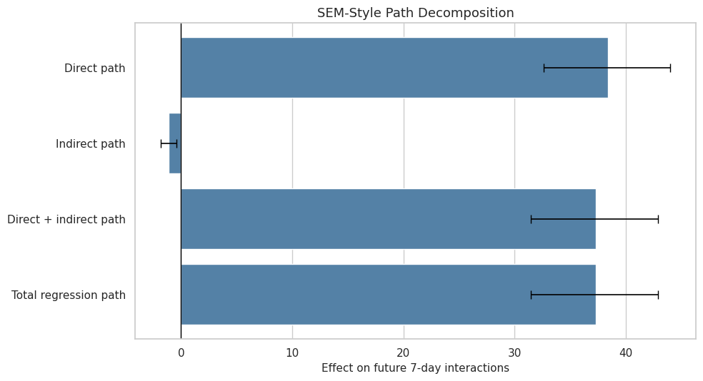

The SEM plot should be read as a path-model summary, not as a new identification strategy. It is useful because it compresses the mediation story into a few path coefficients.

8. Define Cross-Fitted ML Nuisance Models

This cell defines the model families used in the cross-fitted g-computation. The Linear model is the transparent baseline. LightGBM and XGBoost allow nonlinearities and interactions in the nuisance functions.

model_factories = {
    "linear": lambda: LinearRegression(),
    "lightgbm": lambda: LGBMRegressor(
        n_estimators=80,
        learning_rate=0.05,
        num_leaves=24,
        subsample=0.85,
        colsample_bytree=0.85,
        random_state=RANDOM_SEED,
        n_jobs=1,
        verbose=-1,
    ),
    "xgboost": lambda: XGBRegressor(
        n_estimators=80,
        max_depth=3,
        learning_rate=0.05,
        subsample=0.85,
        colsample_bytree=0.85,
        objective="reg:squarederror",
        tree_method="hist",
        random_state=RANDOM_SEED,
        n_jobs=1,
        verbosity=0,
    ),
}

model_summary = pd.DataFrame(
    {
        "model_family": list(model_factories.keys()),
        "role": [
            "transparent benchmark",
            "tree-based nonlinear nuisance model",
            "boosted-tree nonlinear nuisance model",
        ],
    }
)

display(model_summary)

	model_family	role
0	linear	transparent benchmark
1	lightgbm	tree-based nonlinear nuisance model
2	xgboost	boosted-tree nonlinear nuisance model

All three model families estimate the same counterfactual quantities. That keeps the comparison fair: any differences come from nuisance model flexibility, not from changing the causal estimand.

9. Implement Cross-Fitted ML G-Computation

This cell implements group cross-fitting. For each fold, models are trained on some users and evaluated on held-out users. The estimator predicts M(0), M(1), Y(0, M(0)), Y(1, M(0)), and Y(1, M(1)) out of fold, then averages the implied effects.

def treatment_design(covariates, treatment_values):
    design = covariates.copy()
    design.insert(0, TREATMENT, np.asarray(treatment_values, dtype=float))
    return design


def outcome_design(covariates, treatment_values, mediator_values):
    treatment_array = np.asarray(treatment_values, dtype=float)
    mediator_array = np.asarray(mediator_values, dtype=float)
    design = covariates.copy()
    design.insert(0, "A_x_M", treatment_array * mediator_array)
    design.insert(0, MEDIATOR, mediator_array)
    design.insert(0, TREATMENT, treatment_array)
    return design


def fit_with_optional_weight(model, X, y, sample_weight=None):
    try:
        model.fit(X, y, sample_weight=sample_weight)
    except TypeError:
        model.fit(X, y)
    return model


def regression_metrics(y_true, y_pred):
    rmse = mean_squared_error(y_true, y_pred) ** 0.5
    return {
        "rmse": rmse,
        "mae": mean_absolute_error(y_true, y_pred),
        "r2": r2_score(y_true, y_pred),
    }


def crossfit_ml_mediation(model_name, model_factory, outcome_col=PRIMARY_OUTCOME):
    n = len(analysis_panel)
    splitter = GroupKFold(n_splits=N_SPLITS)

    m_hat = np.zeros(n)
    y_hat = np.zeros(n)
    m0 = np.zeros(n)
    m1 = np.zeros(n)
    y_0_m0 = np.zeros(n)
    y_1_m0 = np.zeros(n)
    y_1_m1 = np.zeros(n)
    y_0_m1 = np.zeros(n)

    fold_rows = []
    for fold_id, (train_idx, test_idx) in enumerate(splitter.split(X_covariates, A, groups=groups), start=1):
        X_train = X_covariates.iloc[train_idx]
        X_test = X_covariates.iloc[test_idx]
        A_train = A[train_idx]
        M_train = M[train_idx]
        Y_train = analysis_panel[outcome_col].astype(float).to_numpy()[train_idx]
        W_train = weights[train_idx]

        mediator_model = model_factory()
        outcome_model = model_factory()

        mediator_model = fit_with_optional_weight(
            mediator_model,
            treatment_design(X_train, A_train),
            M_train,
            sample_weight=W_train,
        )
        train_outcome_design = outcome_design(X_train, A_train, M_train)
        outcome_model = fit_with_optional_weight(
            outcome_model,
            train_outcome_design,
            Y_train,
            sample_weight=W_train,
        )

        zeros = np.zeros(len(test_idx))
        ones = np.ones(len(test_idx))
        observed_a = A[test_idx]
        observed_m = M[test_idx]

        m_hat[test_idx] = mediator_model.predict(treatment_design(X_test, observed_a)).clip(0, 1)
        m0[test_idx] = mediator_model.predict(treatment_design(X_test, zeros)).clip(0, 1)
        m1[test_idx] = mediator_model.predict(treatment_design(X_test, ones)).clip(0, 1)

        y_hat[test_idx] = outcome_model.predict(outcome_design(X_test, observed_a, observed_m))
        y_0_m0[test_idx] = outcome_model.predict(outcome_design(X_test, zeros, m0[test_idx]))
        y_1_m0[test_idx] = outcome_model.predict(outcome_design(X_test, ones, m0[test_idx]))
        y_1_m1[test_idx] = outcome_model.predict(outcome_design(X_test, ones, m1[test_idx]))
        y_0_m1[test_idx] = outcome_model.predict(outcome_design(X_test, zeros, m1[test_idx]))

        fold_rows.append(
            {
                "model_family": model_name,
                "outcome": outcome_col,
                "fold": fold_id,
                "train_rows": len(train_idx),
                "test_rows": len(test_idx),
                "test_users": len(np.unique(groups[test_idx])),
            }
        )

    observed_y = analysis_panel[outcome_col].astype(float).to_numpy()
    mediator_metrics = regression_metrics(M, m_hat)
    outcome_metrics = regression_metrics(observed_y, y_hat)

    effects = {
        "model_family": model_name,
        "outcome": outcome_col,
        "outcome_label": "Future 7-day interactions" if outcome_col == PRIMARY_OUTCOME else "Future 7-day play hours",
        "gcomp_total_effect": float(np.mean(y_1_m1 - y_0_m0)),
        "natural_direct_effect": float(np.mean(y_1_m0 - y_0_m0)),
        "natural_indirect_effect": float(np.mean(y_1_m1 - y_1_m0)),
        "reverse_indirect_check": float(np.mean(y_0_m1 - y_0_m0)),
        "mediator_shift": float(np.mean(m1 - m0)),
        "reference_mean": float(np.mean(y_0_m0)),
        "relative_total_effect": float(np.mean(y_1_m1 - y_0_m0) / np.mean(y_0_m0)),
    }

    performance = [
        {"model_family": model_name, "outcome": outcome_col, "target": "mediator", **mediator_metrics},
        {"model_family": model_name, "outcome": outcome_col, "target": "outcome", **outcome_metrics},
    ]

    row_level = pd.DataFrame(
        {
            "user_id": analysis_panel[GROUP_COLUMN].to_numpy(),
            "event_date": analysis_panel["event_date"].to_numpy(),
            "model_family": model_name,
            "outcome": outcome_col,
            "ite_total": y_1_m1 - y_0_m0,
            "ite_direct": y_1_m0 - y_0_m0,
            "ite_indirect": y_1_m1 - y_1_m0,
            "m0_hat": m0,
            "m1_hat": m1,
            "m_hat": m_hat,
            "y_hat": y_hat,
        }
    )

    return effects, performance, pd.DataFrame(fold_rows), row_level

print("Cross-fitted ML mediation function ready.")

Cross-fitted ML mediation function ready.

The row-level output is useful for heterogeneity. Each held-out row receives an estimated total, direct, and indirect effect, which can then be summarized by user segments.

10. Run Cross-Fitted ML Mediation

This cell runs the cross-fitted estimator for Linear Regression, LightGBM, and XGBoost. It estimates the primary future-interaction outcome and a secondary future-play-hours outcome.

ml_effect_rows = []
ml_performance_rows = []
fold_summaries = []
row_level_effect_frames = []

for outcome_col in [PRIMARY_OUTCOME, SECONDARY_OUTCOME]:
    for model_name, model_factory in model_factories.items():
        effects, performance, folds, row_level = crossfit_ml_mediation(
            model_name,
            model_factory,
            outcome_col=outcome_col,
        )
        ml_effect_rows.append(effects)
        ml_performance_rows.extend(performance)
        fold_summaries.append(folds)
        row_level_effect_frames.append(row_level)

ml_effects = pd.DataFrame(ml_effect_rows)
ml_performance = pd.DataFrame(ml_performance_rows)
ml_fold_summary = pd.concat(fold_summaries, ignore_index=True)
row_level_effects = pd.concat(row_level_effect_frames, ignore_index=True)

display(ml_effects.round(4))
display(ml_performance.round(4))

	model_family	outcome	outcome_label	gcomp_total_effect	natural_direct_effect	natural_indirect_effect	reverse_indirect_check	mediator_shift	reference_mean	relative_total_effect
0	linear	Y_future_interactions	Future 7-day interactions	37.3421	38.6464	-1.3043	-0.9904	0.0231	322.8968	0.1156
1	lightgbm	Y_future_interactions	Future 7-day interactions	3.2069	3.2652	-0.0583	-0.0137	0.0184	339.1834	0.0095
2	xgboost	Y_future_interactions	Future 7-day interactions	2.6829	2.7279	-0.0450	-0.0294	0.0138	339.7969	0.0079
3	linear	Y_future_play_hours	Future 7-day play hours	0.0786	0.0745	0.0042	0.0021	0.0231	0.7480	0.1051
4	lightgbm	Y_future_play_hours	Future 7-day play hours	0.0076	0.0030	0.0046	0.0046	0.0184	0.8177	0.0093
5	xgboost	Y_future_play_hours	Future 7-day play hours	0.0062	0.0034	0.0028	0.0027	0.0138	0.8230	0.0075

	model_family	outcome	target	rmse	mae	r2
0	linear	Y_future_interactions	mediator	0.1015	0.0703	0.1878
1	linear	Y_future_interactions	outcome	96.6374	71.1050	0.7129
2	lightgbm	Y_future_interactions	mediator	0.0875	0.0629	0.3959
3	lightgbm	Y_future_interactions	outcome	66.7067	47.0941	0.8632
4	xgboost	Y_future_interactions	mediator	0.0870	0.0625	0.4026
5	xgboost	Y_future_interactions	outcome	66.0357	46.7289	0.8659
6	linear	Y_future_play_hours	mediator	0.1015	0.0703	0.1878
7	linear	Y_future_play_hours	outcome	0.3609	0.2428	0.4056
8	lightgbm	Y_future_play_hours	mediator	0.0875	0.0629	0.3959
9	lightgbm	Y_future_play_hours	outcome	0.2388	0.1672	0.7398
10	xgboost	Y_future_play_hours	mediator	0.0870	0.0625	0.4026
11	xgboost	Y_future_play_hours	outcome	0.2383	0.1694	0.7409

The model comparison is now cross-fitted. If the flexible models preserve the positive total effect and small mediated pathway, the earlier story is less likely to be an artifact of linear functional form.

11. Plot Cross-Fitted Model Comparison

This cell visualizes total, direct, and indirect effects across model families for the primary outcome. The plot uses the cross-fitted estimates from held-out users.

primary_ml_plot = ml_effects.query("outcome == @PRIMARY_OUTCOME").melt(
    id_vars=["model_family"],
    value_vars=["gcomp_total_effect", "natural_direct_effect", "natural_indirect_effect"],
    var_name="effect_type",
    value_name="estimate",
)
primary_ml_plot["effect_label"] = primary_ml_plot["effect_type"].map(
    {
        "gcomp_total_effect": "Total",
        "natural_direct_effect": "Direct",
        "natural_indirect_effect": "Indirect",
    }
)
primary_ml_plot["model_label"] = primary_ml_plot["model_family"].str.upper()

fig, ax = plt.subplots(figsize=(11, 6))
sns.barplot(data=primary_ml_plot, x="estimate", y="model_label", hue="effect_label", ax=ax)
ax.axvline(0, color="black", linewidth=1)
ax.set_title("Cross-Fitted ML Mediation Effect Comparison")
ax.set_xlabel("Effect on future 7-day interactions")
ax.set_ylabel("Model family")
plt.tight_layout()
fig.savefig(FIGURE_DIR / "21_crossfit_ml_effect_comparison.png", dpi=160, bbox_inches="tight")
plt.show()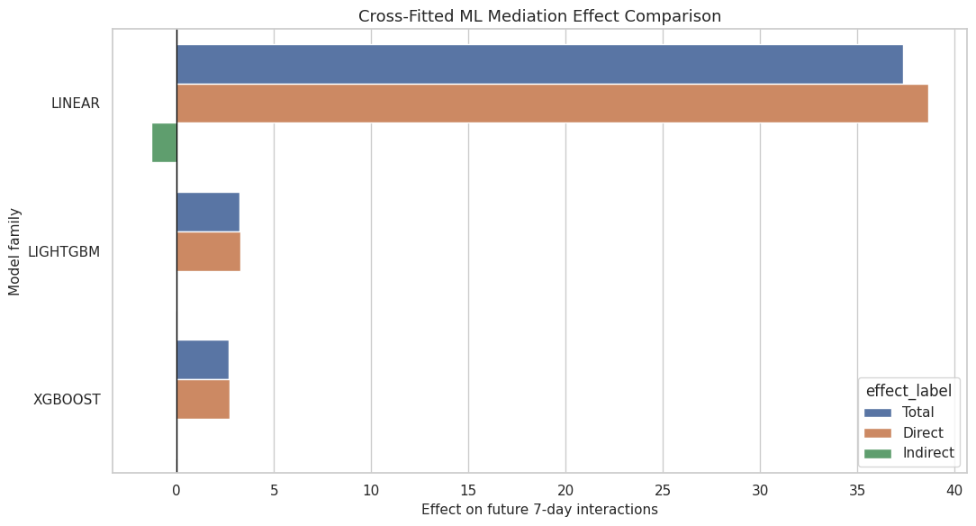

This comparison is the main advanced-model result. Agreement across Linear, LightGBM, and XGBoost is more reassuring than any one model alone.

12. Compare Predictive Performance

This cell compares out-of-fold predictive performance for the mediator and outcome nuisance models. Stronger prediction does not automatically mean a better causal estimate, but very weak prediction can make counterfactual estimates unstable.

performance_plot = ml_performance.copy()
performance_plot["model_label"] = performance_plot["model_family"].str.upper()
performance_plot["target_label"] = performance_plot["target"].str.title()
performance_plot["outcome_label"] = performance_plot["outcome"].map(
    {PRIMARY_OUTCOME: "Future interactions", SECONDARY_OUTCOME: "Future play hours"}
)

fig, axes = plt.subplots(1, 2, figsize=(14, 5))
for ax, metric in zip(axes, ["rmse", "r2"]):
    sns.barplot(
        data=performance_plot.query("outcome == @PRIMARY_OUTCOME"),
        x=metric,
        y="model_label",
        hue="target_label",
        ax=ax,
    )
    ax.set_title(f"Primary Outcome Nuisance {metric.upper()}")
    ax.set_xlabel(metric.upper())
    ax.set_ylabel("Model family")
plt.tight_layout()
fig.savefig(FIGURE_DIR / "22_crossfit_nuisance_performance.png", dpi=160, bbox_inches="tight")
plt.show()

display(ml_performance.round(4))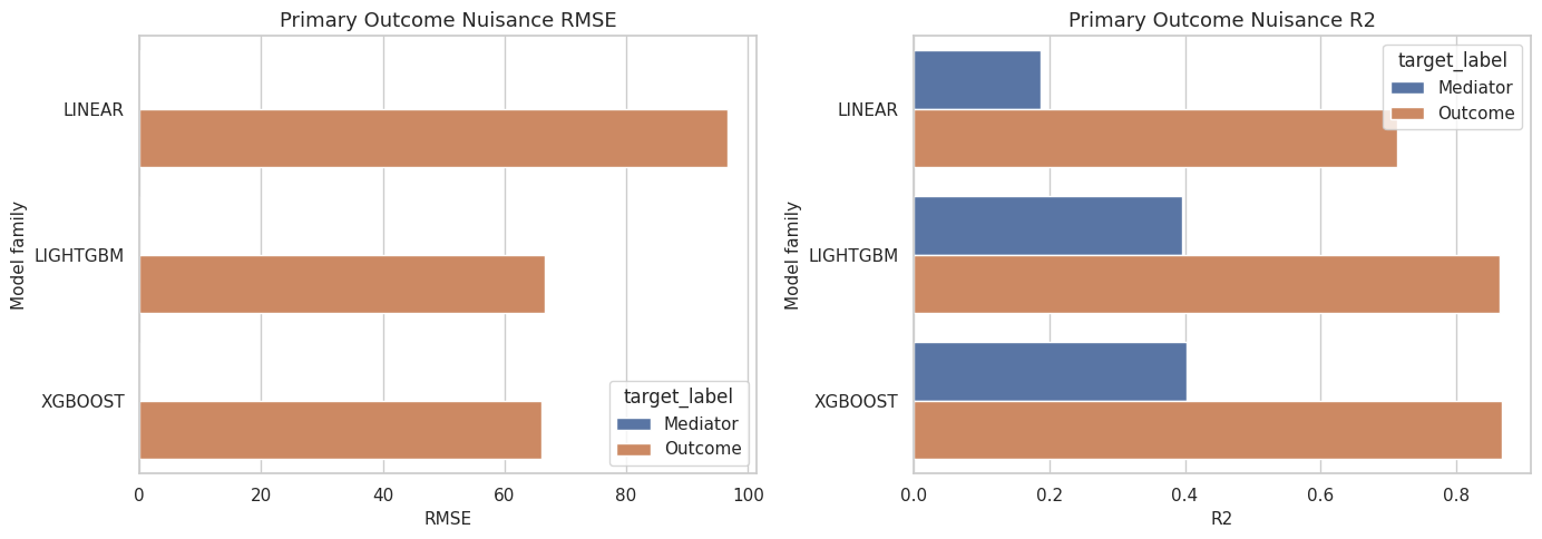

	model_family	outcome	target	rmse	mae	r2
0	linear	Y_future_interactions	mediator	0.1015	0.0703	0.1878
1	linear	Y_future_interactions	outcome	96.6374	71.1050	0.7129
2	lightgbm	Y_future_interactions	mediator	0.0875	0.0629	0.3959
3	lightgbm	Y_future_interactions	outcome	66.7067	47.0941	0.8632
4	xgboost	Y_future_interactions	mediator	0.0870	0.0625	0.4026
5	xgboost	Y_future_interactions	outcome	66.0357	46.7289	0.8659
6	linear	Y_future_play_hours	mediator	0.1015	0.0703	0.1878
7	linear	Y_future_play_hours	outcome	0.3609	0.2428	0.4056
8	lightgbm	Y_future_play_hours	mediator	0.0875	0.0629	0.3959
9	lightgbm	Y_future_play_hours	outcome	0.2388	0.1672	0.7398
10	xgboost	Y_future_play_hours	mediator	0.0870	0.0625	0.4026
11	xgboost	Y_future_play_hours	outcome	0.2383	0.1694	0.7409

The performance table helps explain model behavior. If a flexible model changes the effect estimate but does not improve held-out performance, that change deserves caution.

13. Heterogeneity from Cross-Fitted Effects

This cell uses LightGBM’s row-level cross-fitted effects to summarize heterogeneity. The groups are based on pre-treatment information: prior activity, prior satisfaction, prior discovery, and user activity degree.

heterogeneity_base = analysis_panel[[
    "user_id",
    "event_date",
    "prior_3day_interactions",
    "prior_3day_high_satisfaction_share",
    "prior_3day_discovery_candidate_share",
    "user_active_degree",
]].copy()

heterogeneity_base["prior_activity_group"] = pd.qcut(
    heterogeneity_base["prior_3day_interactions"].rank(method="first"),
    q=3,
    labels=["low prior activity", "medium prior activity", "high prior activity"],
)
heterogeneity_base["prior_satisfaction_group"] = pd.qcut(
    heterogeneity_base["prior_3day_high_satisfaction_share"].rank(method="first"),
    q=3,
    labels=["low prior satisfaction", "medium prior satisfaction", "high prior satisfaction"],
)
heterogeneity_base["prior_discovery_group"] = pd.qcut(
    heterogeneity_base["prior_3day_discovery_candidate_share"].rank(method="first"),
    q=3,
    labels=["low prior discovery", "medium prior discovery", "high prior discovery"],
)

lightgbm_row_effects = row_level_effects.query(
    "model_family == 'lightgbm' and outcome == @PRIMARY_OUTCOME"
).merge(
    heterogeneity_base,
    on=["user_id", "event_date"],
    how="left",
)

heterogeneity_rows = []
for segment_col in ["prior_activity_group", "prior_satisfaction_group", "prior_discovery_group", "user_active_degree"]:
    summary = (
        lightgbm_row_effects.groupby(segment_col, observed=True)
        .agg(
            user_days=("user_id", "size"),
            users=("user_id", "nunique"),
            total_effect=("ite_total", "mean"),
            direct_effect=("ite_direct", "mean"),
            indirect_effect=("ite_indirect", "mean"),
            mediator_shift=("m1_hat", "mean"),
        )
        .reset_index()
        .rename(columns={segment_col: "segment_value"})
    )
    summary["segment"] = segment_col
    heterogeneity_rows.append(summary)

heterogeneity_effects = pd.concat(heterogeneity_rows, ignore_index=True)
# Convert mediator_shift from average M1 to the segment-level treatment-induced shift.
for segment_col in ["prior_activity_group", "prior_satisfaction_group", "prior_discovery_group", "user_active_degree"]:
    mask = heterogeneity_effects["segment"].eq(segment_col)
    segment_shift = (
        lightgbm_row_effects.groupby(segment_col, observed=True)
        .apply(lambda g: (g["m1_hat"] - g["m0_hat"]).mean(), include_groups=False)
        .reset_index(name="true_mediator_shift")
        .rename(columns={segment_col: "segment_value"})
    )
    heterogeneity_effects.loc[mask, "mediator_shift"] = heterogeneity_effects.loc[mask].merge(
        segment_shift, on="segment_value", how="left"
    )["true_mediator_shift"].to_numpy()

display(heterogeneity_effects.round(4))

	segment_value	user_days	users	total_effect	direct_effect	indirect_effect	mediator_shift	segment
0	low prior activity	2733	133	2.1266	2.3286	-0.2021	0.0195	prior_activity_group
1	medium prior activity	2733	133	3.9690	4.0530	-0.0841	0.0177	prior_activity_group
2	high prior activity	2733	133	3.5253	3.4140	0.1112	0.0180	prior_activity_group
3	low prior satisfaction	2733	133	2.9903	2.8696	0.1208	0.0165	prior_satisfaction_group
4	medium prior satisfaction	2733	130	3.5907	3.7333	-0.1426	0.0158	prior_satisfaction_group
5	high prior satisfaction	2733	113	3.0398	3.1928	-0.1530	0.0229	prior_satisfaction_group
6	low prior discovery	2733	133	2.0592	2.1656	-0.1064	0.0184	prior_discovery_group
7	medium prior discovery	2733	133	3.3925	3.3729	0.0196	0.0166	prior_discovery_group
8	high prior discovery	2733	133	4.1691	4.2572	-0.0881	0.0201	prior_discovery_group
9	UNKNOWN	184	3	4.4181	4.5911	-0.1731	0.0241	user_active_degree
10	full_active	7133	115	3.1915	3.2485	-0.0570	0.0181	user_active_degree
11	high_active	882	15	3.0788	3.1241	-0.0453	0.0195	user_active_degree

The heterogeneity table asks where the discovery effect is largest. Because these are subgroup summaries of cross-fitted predictions, they are descriptive signals for product targeting rather than separate randomized subgroup effects.

14. Plot Heterogeneous Effects

This cell plots LightGBM total effects by segment. It focuses on total effects because those are the most stable quantities in the earlier robustness checks.

heterogeneity_plot = heterogeneity_effects.copy()
heterogeneity_plot["segment_label"] = heterogeneity_plot["segment"].str.replace("_", " ").str.title()
heterogeneity_plot["segment_value"] = heterogeneity_plot["segment_value"].astype(str)

fig, axes = plt.subplots(2, 2, figsize=(15, 10))
axes = axes.flatten()
for ax, segment in zip(axes, heterogeneity_plot["segment"].unique()):
    current = heterogeneity_plot.query("segment == @segment").copy()
    sns.barplot(data=current, x="total_effect", y="segment_value", color="steelblue", ax=ax)
    ax.axvline(0, color="black", linewidth=1)
    ax.set_title(segment.replace("_", " ").title())
    ax.set_xlabel("LightGBM total effect on future interactions")
    ax.set_ylabel("")
plt.tight_layout()
fig.savefig(FIGURE_DIR / "23_lightgbm_heterogeneous_effects.png", dpi=160, bbox_inches="tight")
plt.show()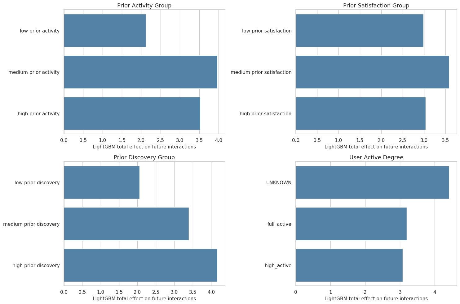

The heterogeneity plot makes the advanced notebook more product-relevant. It shows where the model expects discovery exposure to matter more or less.

15. Train Full Tree Models for Feature Importance

This cell trains full-sample LightGBM and XGBoost nuisance models for feature importance only. These models are not used for effect estimates; the effect estimates above are cross-fitted. The goal here is model auditability.

feature_importance_rows = []
full_design_m = treatment_design(X_covariates, A)
full_design_y = outcome_design(X_covariates, A, M)

importance_model_specs = [
    ("lightgbm", LGBMRegressor(
        n_estimators=120,
        learning_rate=0.05,
        num_leaves=24,
        subsample=0.85,
        colsample_bytree=0.85,
        random_state=RANDOM_SEED,
        n_jobs=1,
        verbose=-1,
    )),
    ("xgboost", XGBRegressor(
        n_estimators=120,
        max_depth=3,
        learning_rate=0.05,
        subsample=0.85,
        colsample_bytree=0.85,
        objective="reg:squarederror",
        tree_method="hist",
        random_state=RANDOM_SEED,
        n_jobs=1,
        verbosity=0,
    )),
]

for model_family, model in importance_model_specs:
    mediator_model = clone(model)
    outcome_model = clone(model)
    fit_with_optional_weight(mediator_model, full_design_m, M, sample_weight=weights)
    fit_with_optional_weight(outcome_model, full_design_y, Y, sample_weight=weights)

    for target_name, fitted_model, design in [
        ("mediator", mediator_model, full_design_m),
        ("outcome", outcome_model, full_design_y),
    ]:
        importances = getattr(fitted_model, "feature_importances_", None)
        if importances is None:
            continue
        current = pd.DataFrame(
            {
                "model_family": model_family,
                "target": target_name,
                "feature": design.columns,
                "importance": importances,
            }
        )
        current["importance_share"] = current["importance"] / current["importance"].sum()
        feature_importance_rows.append(current)

feature_importance = pd.concat(feature_importance_rows, ignore_index=True)
top_feature_importance = (
    feature_importance.sort_values(["model_family", "target", "importance"], ascending=[True, True, False])
    .groupby(["model_family", "target"], group_keys=False)
    .head(12)
    .reset_index(drop=True)
)

display(top_feature_importance.round(4))

	model_family	target	feature	importance	importance_share
0	lightgbm	mediator	calendar_day_index	297.0000	0.1076
1	lightgbm	mediator	prior_3day_high_satisfaction_share	260.0000	0.0942
2	lightgbm	mediator	lag_1_high_satisfaction_share	249.0000	0.0902
3	lightgbm	mediator	prior_3day_discovery_candidate_share	187.0000	0.0678
4	lightgbm	mediator	onehot_feat8	147.0000	0.0533
5	lightgbm	mediator	lag_1_valid_play_share	137.0000	0.0496
6	lightgbm	mediator	prior_3day_valid_play_share	122.0000	0.0442
7	lightgbm	mediator	onehot_feat3	118.0000	0.0428
8	lightgbm	mediator	register_days	111.0000	0.0402
9	lightgbm	mediator	prior_3day_total_play_duration_sec	108.0000	0.0391
10	lightgbm	mediator	lag_1_total_play_duration_sec	103.0000	0.0373
11	lightgbm	mediator	A_high_discovery	101.0000	0.0366
12	lightgbm	outcome	calendar_day_index	592.0000	0.2145
13	lightgbm	outcome	onehot_feat8	187.0000	0.0678
14	lightgbm	outcome	prior_3day_discovery_candidate_share	180.0000	0.0652
15	lightgbm	outcome	prior_3day_interactions	157.0000	0.0569
16	lightgbm	outcome	register_days	148.0000	0.0536
17	lightgbm	outcome	onehot_feat7	126.0000	0.0457
18	lightgbm	outcome	prior_3day_high_satisfaction_share	121.0000	0.0438
19	lightgbm	outcome	onehot_feat3	120.0000	0.0435
20	lightgbm	outcome	follow_user_num	108.0000	0.0391
21	lightgbm	outcome	prior_3day_total_play_duration_sec	105.0000	0.0380
22	lightgbm	outcome	prior_3day_valid_play_share	103.0000	0.0373
23	lightgbm	outcome	fans_user_num	87.0000	0.0315
24	xgboost	mediator	prior_3day_high_satisfaction_share	0.1697	0.1697
25	xgboost	mediator	lag_1_high_satisfaction_share	0.0686	0.0686
26	xgboost	mediator	lag_1_valid_play_share	0.0570	0.0570
27	xgboost	mediator	prior_3day_valid_play_share	0.0436	0.0436
28	xgboost	mediator	lag_1_interactions	0.0432	0.0432
29	xgboost	mediator	onehot_feat11	0.0416	0.0416
30	xgboost	mediator	fans_user_num_range_1_10	0.0381	0.0381
31	xgboost	mediator	user_active_degree_high_active	0.0330	0.0330
32	xgboost	mediator	prior_3day_active_day	0.0312	0.0312
33	xgboost	mediator	onehot_feat6	0.0262	0.0262
34	xgboost	mediator	lag_1_total_play_duration_sec	0.0261	0.0261
35	xgboost	mediator	A_high_discovery	0.0227	0.0227
36	xgboost	outcome	calendar_day_index	0.3093	0.3093
37	xgboost	outcome	prior_3day_active_day	0.1905	0.1905
38	xgboost	outcome	prior_3day_discovery_candidate_share	0.1517	0.1517
39	xgboost	outcome	prior_3day_interactions	0.0373	0.0373
40	xgboost	outcome	lag_1_interactions	0.0202	0.0202
41	xgboost	outcome	lag_1_discovery_candidate_share	0.0190	0.0190
42	xgboost	outcome	recent_activity_score	0.0169	0.0169
43	xgboost	outcome	user_active_degree_high_active	0.0161	0.0161
44	xgboost	outcome	prior_3day_total_play_duration_sec	0.0145	0.0145
45	xgboost	outcome	register_days_range_61_90	0.0141	0.0141
46	xgboost	outcome	fans_user_num	0.0136	0.0136
47	xgboost	outcome	onehot_feat14	0.0117	0.0117

The feature-importance audit helps reveal whether models are mostly using treatment, mediator, calendar time, prior activity, or profile signals. That matters because an advanced model can look impressive while leaning heavily on confounding proxies.

16. Plot Feature Importance

This cell plots the top features for the LightGBM nuisance models. LightGBM is used here because its importances are usually stable and easy to read.

importance_plot = top_feature_importance.query("model_family == 'lightgbm'").copy()
importance_plot["feature_label"] = importance_plot["feature"].str.replace("_", " ").str.slice(0, 45)
importance_plot["target_label"] = importance_plot["target"].str.title()

fig, axes = plt.subplots(1, 2, figsize=(16, 6))
for ax, target in zip(axes, ["mediator", "outcome"]):
    current = importance_plot.query("target == @target").sort_values("importance", ascending=True)
    sns.barplot(data=current, x="importance", y="feature_label", color="steelblue", ax=ax)
    ax.set_title(f"LightGBM {target.title()} Model Features")
    ax.set_xlabel("Feature importance")
    ax.set_ylabel("")
plt.tight_layout()
fig.savefig(FIGURE_DIR / "24_lightgbm_feature_importance.png", dpi=160, bbox_inches="tight")
plt.show()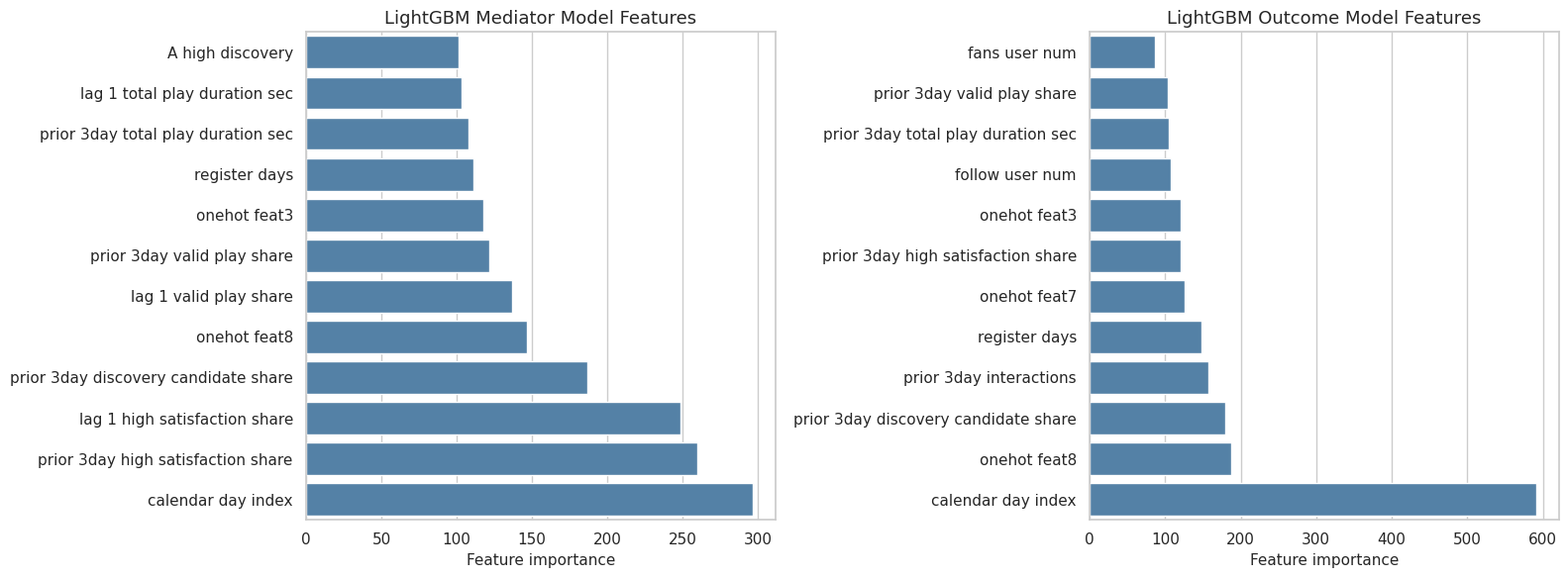

The feature plot is an audit layer, not an explanation of causality. It tells us what the prediction functions used, which is useful for debugging and for communicating model behavior.

17. Advanced Model Summary

This cell combines the linear g-computation result from notebook 04, SEM-style paths, and cross-fitted ML estimates into one comparison table. The table is the main handoff to the final report.

linear_reference = effect_summary.query(
    "outcome == @PRIMARY_OUTCOME and estimand in ['gcomp_total_effect', 'natural_direct_effect', 'natural_indirect_effect']"
).pivot_table(index="outcome", columns="estimand", values="estimate").reset_index()
linear_reference["model_family"] = "linear_reference_from_notebook_04"
linear_reference = linear_reference.rename(
    columns={
        "gcomp_total_effect": "total_effect",
        "natural_direct_effect": "direct_effect",
        "natural_indirect_effect": "indirect_effect",
    }
)[["model_family", "total_effect", "direct_effect", "indirect_effect"]]

sem_reference = pd.DataFrame(
    [
        {
            "model_family": "sem_style_path_model",
            "total_effect": sem_path_results.loc[0, "total_path_c_prime_plus_indirect"],
            "direct_effect": sem_path_results.loc[0, "c_prime_A_to_Y"],
            "indirect_effect": sem_path_results.loc[0, "indirect_alpha_beta"],
        }
    ]
)

ml_reference = ml_effects.query("outcome == @PRIMARY_OUTCOME").rename(
    columns={
        "gcomp_total_effect": "total_effect",
        "natural_direct_effect": "direct_effect",
        "natural_indirect_effect": "indirect_effect",
    }
)[["model_family", "total_effect", "direct_effect", "indirect_effect", "mediator_shift", "relative_total_effect"]]

advanced_model_summary = pd.concat(
    [linear_reference, sem_reference, ml_reference],
    ignore_index=True,
    sort=False,
)
advanced_model_summary["indirect_to_total_ratio"] = (
    advanced_model_summary["indirect_effect"] / advanced_model_summary["total_effect"].replace(0, np.nan)
)
advanced_model_summary["total_effect_positive"] = advanced_model_summary["total_effect"] > 0
advanced_model_summary["indirect_effect_small_abs_lt_5"] = advanced_model_summary["indirect_effect"].abs() < 5

display(advanced_model_summary.round(4))

	model_family	total_effect	direct_effect	indirect_effect	mediator_shift	relative_total_effect	indirect_to_total_ratio	total_effect_positive	indirect_effect_small_abs_lt_5
0	linear_reference_from_notebook_04	37.2781	38.5858	-1.3077	NaN	NaN	-0.0351	True	True
1	sem_style_path_model	37.3139	38.4311	-1.1172	NaN	NaN	-0.0299	True	True
2	linear	37.3421	38.6464	-1.3043	0.0231	0.1156	-0.0349	True	True
3	lightgbm	3.2069	3.2652	-0.0583	0.0184	0.0095	-0.0182	True	True
4	xgboost	2.6829	2.7279	-0.0450	0.0138	0.0079	-0.0168	True	True

The comparison table answers the advanced-model question directly. If the total effect is positive across model families and the indirect effect remains small, the notebook 04 result is strengthened.

18. Plot Advanced Model Summary

This cell plots total, direct, and indirect effects across the reference, SEM-style, and cross-fitted ML approaches.

summary_plot = advanced_model_summary.melt(
    id_vars=["model_family"],
    value_vars=["total_effect", "direct_effect", "indirect_effect"],
    var_name="effect_type",
    value_name="estimate",
)
summary_plot["effect_label"] = summary_plot["effect_type"].map(
    {
        "total_effect": "Total",
        "direct_effect": "Direct",
        "indirect_effect": "Indirect",
    }
)
summary_plot["model_label"] = summary_plot["model_family"].str.replace("_", " ").str.title()

fig, ax = plt.subplots(figsize=(13, 7))
sns.barplot(data=summary_plot, x="estimate", y="model_label", hue="effect_label", ax=ax)
ax.axvline(0, color="black", linewidth=1)
ax.set_title("Advanced Model Comparison for Discovery Mediation")
ax.set_xlabel("Effect on future 7-day interactions")
ax.set_ylabel("Model approach")
plt.tight_layout()
fig.savefig(FIGURE_DIR / "25_advanced_model_summary.png", dpi=160, bbox_inches="tight")
plt.show()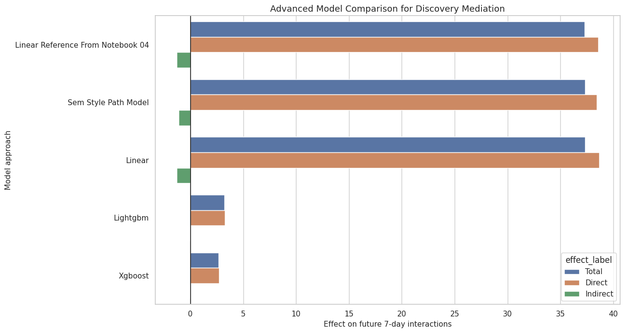

This final figure is the high-level advanced-model takeaway. It lets a reader see whether the main story depends on the modeling approach.

19. Save Advanced Model Artifacts

This cell saves the SEM path results, bootstrap path samples, ML effect estimates, model performance, heterogeneity table, feature importance table, and advanced summary table.

sem_path_summary.to_csv(SEM_PATH_OUTPUT, index=False)
sem_bootstrap.to_csv(SEM_BOOTSTRAP_OUTPUT, index=False)
ml_effects.to_csv(ML_EFFECTS_OUTPUT, index=False)
ml_performance.to_csv(ML_PERFORMANCE_OUTPUT, index=False)
heterogeneity_effects.to_csv(HETEROGENEITY_OUTPUT, index=False)
feature_importance.to_csv(FEATURE_IMPORTANCE_OUTPUT, index=False)
advanced_model_summary.to_csv(ADVANCED_SUMMARY_OUTPUT, index=False)

sem_path_summary.to_csv(TABLE_DIR / "advanced_sem_path_results.csv", index=False)
ml_effects.to_csv(TABLE_DIR / "advanced_ml_effects.csv", index=False)
ml_performance.to_csv(TABLE_DIR / "advanced_ml_performance.csv", index=False)
heterogeneity_effects.to_csv(TABLE_DIR / "advanced_heterogeneity.csv", index=False)
top_feature_importance.to_csv(TABLE_DIR / "advanced_feature_importance_top.csv", index=False)
advanced_model_summary.to_csv(TABLE_DIR / "advanced_model_summary.csv", index=False)

saved_outputs = pd.DataFrame(
    {
        "artifact": [
            "sem_path_results",
            "sem_bootstrap",
            "ml_effects",
            "ml_performance",
            "heterogeneity_effects",
            "feature_importance",
            "advanced_model_summary",
        ],
        "path": [
            str(SEM_PATH_OUTPUT),
            str(SEM_BOOTSTRAP_OUTPUT),
            str(ML_EFFECTS_OUTPUT),
            str(ML_PERFORMANCE_OUTPUT),
            str(HETEROGENEITY_OUTPUT),
            str(FEATURE_IMPORTANCE_OUTPUT),
            str(ADVANCED_SUMMARY_OUTPUT),
        ],
    }
)

display(saved_outputs)

	artifact	path
0	sem_path_results	/home/apex/Documents/ranking_sys/data/processed/kuairec_discovery_quality_sem_path_results.csv
1	sem_bootstrap	/home/apex/Documents/ranking_sys/data/processed/kuairec_discovery_quality_sem_bootstrap.csv
2	ml_effects	/home/apex/Documents/ranking_sys/data/processed/kuairec_discovery_quality_advanced_ml_effects.csv
3	ml_performance	/home/apex/Documents/ranking_sys/data/processed/kuairec_discovery_quality_advanced_ml_performance.csv
4	heterogeneity_effects	/home/apex/Documents/ranking_sys/data/processed/kuairec_discovery_quality_advanced_heterogeneity.csv
5	feature_importance	/home/apex/Documents/ranking_sys/data/processed/kuairec_discovery_quality_advanced_feature_importance.csv
6	advanced_model_summary	/home/apex/Documents/ranking_sys/data/processed/kuairec_discovery_quality_advanced_model_summary.csv

The saved tables give the final report enough material to compare simple and advanced estimators without rerunning the models.

20. Notebook Takeaways

This notebook added advanced model checks to the discovery-quality mediation workflow:

• SEM-style path modeling gives a compact path-coefficient version of the mediation story.
• Cross-fitted Linear, LightGBM, and XGBoost nuisance models test whether the decomposition survives nonlinear prediction functions.
• Heterogeneity summaries show where discovery exposure appears more or less valuable.
• Feature-importance tables audit which variables the tree-based nuisance models rely on.
• The final comparison table tells the final report whether the main result is stable across modeling approaches.

The next notebook should be the final report and figures notebook, using the simple, robustness, and advanced-model outputs together.