from pathlib import Path
import os
import warnings

os.environ.setdefault("OMP_NUM_THREADS", "1")
os.environ.setdefault("OPENBLAS_NUM_THREADS", "1")
os.environ.setdefault("MKL_NUM_THREADS", "1")
os.environ.setdefault("NUMEXPR_NUM_THREADS", "1")

import numpy as np
import pandas as pd
import seaborn as sns
import matplotlib.pyplot as plt
from IPython.display import display
from sklearn.linear_model import LinearRegression, LogisticRegression
from sklearn.pipeline import make_pipeline
from sklearn.preprocessing import StandardScaler

warnings.filterwarnings("ignore", category=FutureWarning)

sns.set_theme(style="whitegrid", context="notebook")
plt.rcParams["figure.figsize"] = (11, 6)
plt.rcParams["axes.titlesize"] = 13
plt.rcParams["axes.labelsize"] = 11
pd.set_option("display.max_columns", 180)
pd.set_option("display.max_colwidth", 140)

PROJECT_ROOT = Path.cwd().resolve()
while not (PROJECT_ROOT / "data").exists() and PROJECT_ROOT.parent != PROJECT_ROOT:
    PROJECT_ROOT = PROJECT_ROOT.parent

PROCESSED_DIR = PROJECT_ROOT / "data" / "processed"
NOTEBOOK_DIR = PROJECT_ROOT / "notebooks" / "discovery_quality_mediation"
WRITEUP_DIR = NOTEBOOK_DIR / "writeup"
FIGURE_DIR = WRITEUP_DIR / "figures"
TABLE_DIR = WRITEUP_DIR / "tables"

FIGURE_DIR.mkdir(parents=True, exist_ok=True)
TABLE_DIR.mkdir(parents=True, exist_ok=True)

ANALYSIS_PANEL_INPUT = PROCESSED_DIR / "kuairec_discovery_quality_mediation_analysis_panel.parquet"
EFFECT_SUMMARY_INPUT = PROCESSED_DIR / "kuairec_discovery_quality_effect_summary.csv"
ASSUMPTION_CHECKS_INPUT = PROCESSED_DIR / "kuairec_discovery_quality_assumption_checks.csv"

THRESHOLD_OUTPUT = PROCESSED_DIR / "kuairec_discovery_quality_robustness_thresholds.csv"
MEDIATOR_OUTPUT = PROCESSED_DIR / "kuairec_discovery_quality_robustness_mediators.csv"
MODEL_SENSITIVITY_OUTPUT = PROCESSED_DIR / "kuairec_discovery_quality_model_sensitivity.csv"
CONTINUOUS_OUTPUT = PROCESSED_DIR / "kuairec_discovery_quality_continuous_score_sensitivity.csv"
PLACEBO_OUTPUT = PROCESSED_DIR / "kuairec_discovery_quality_placebo_checks.csv"
ROBUSTNESS_SUMMARY_OUTPUT = PROCESSED_DIR / "kuairec_discovery_quality_robustness_summary.csv"
LIMITATIONS_OUTPUT = PROCESSED_DIR / "kuairec_discovery_quality_limitations.csv"Robustness and Sensitivity for Discovery Quality Mediation
The previous notebook estimated the main discovery-quality mediation result: high discovery exposure was associated with higher future interaction volume, while the satisfaction-depth mediated pathway was small and slightly negative for the primary interaction-count outcome.
This notebook asks whether that story is fragile.
A good causal portfolio notebook should not stop after one preferred specification. It should ask what happens when reasonable choices change:
- Does the result survive different high-discovery thresholds?
- Does it depend on one particular satisfaction mediator definition?
- Does it look similar for future play time and active days?
- Does it change under weighted versus unweighted models?
- Does it depend on including a treatment-mediator interaction?
- Is the result mostly a calendar-time or pre-period activity artifact?
The goal is not to prove the observational design is perfect. The goal is to show what is stable, what is sensitive, and what a careful reader should trust only with caveats.
1. Load Libraries and Paths
This cell imports the libraries used for robustness modeling and plotting. It also defines all inputs from the previous notebooks and all outputs created here.
The thread limits keep the notebook predictable on a laptop or shared environment. This notebook runs many small linear models, so it does not need aggressive parallel math libraries.
2. Load the Analysis Panel and Main Results
This cell loads the mediation analysis panel and the effect summary from notebook 04. The effect summary is the reference point for every stress test in this notebook.
analysis_panel = pd.read_parquet(ANALYSIS_PANEL_INPUT)
effect_summary = pd.read_csv(EFFECT_SUMMARY_INPUT)
assumption_checks = pd.read_csv(ASSUMPTION_CHECKS_INPUT)

load_summary = pd.DataFrame(
    {
        "artifact": ["analysis_panel", "effect_summary", "assumption_checks"],
        "rows": [len(analysis_panel), len(effect_summary), len(assumption_checks)],
        "columns": [analysis_panel.shape[1], effect_summary.shape[1], assumption_checks.shape[1]],
    }
)

main_primary = effect_summary.query(
    "outcome == 'Y_future_interactions' and estimand in ['gcomp_total_effect', 'natural_direct_effect', 'natural_indirect_effect']"
).copy()

display(load_summary)
display(main_primary[["outcome_label", "estimand", "estimate", "ci_95_lower", "ci_95_upper", "relative_effect"]].round(4))| artifact | rows | columns | |
|---|---|---|---|
| 0 | analysis_panel | 8199 | 103 |
| 1 | effect_summary | 21 | 12 |
| 2 | assumption_checks | 6 | 5 |
| outcome_label | estimand | estimate | ci_95_lower | ci_95_upper | relative_effect | |
|---|---|---|---|---|---|---|
| 2 | Future 7-day interactions | gcomp_total_effect | 37.2781 | 32.2444 | 42.8135 | 0.1152 |
| 3 | Future 7-day interactions | natural_direct_effect | 38.5858 | 33.3634 | 43.7154 | 0.1192 |
| 4 | Future 7-day interactions | natural_indirect_effect | -1.3077 | -2.3047 | -0.4290 | -0.0036 |
The main result is the anchor: a positive total effect on future interactions, a direct effect of similar size, and a small negative indirect pathway through the satisfaction-depth metric. The rest of this notebook checks how stable that pattern is.
3. Define Outcomes, Mediators, and Controls
This cell defines the variable sets used across robustness checks. The rich controls mirror earlier notebooks. The simple controls are intentionally smaller and help answer whether the result is only produced by a large adjustment set.
PRIMARY_OUTCOME = "Y_future_interactions"
OUTCOME_COLUMNS = ["Y_future_interactions", "Y_future_active_days", "Y_future_play_hours"]
OUTCOME_LABELS = {
    "Y_future_interactions": "Future 7-day interactions",
    "Y_future_active_days": "Future 7-day active days",
    "Y_future_play_hours": "Future 7-day play hours",
}
BASE_TREATMENT = "A_high_discovery"
BASE_MEDIATOR = "M_satisfaction_depth"
DISCOVERY_SCORE = "discovery_breadth_score"

base_numeric_covariates = [
    "calendar_day_index",
    "lag_1_active_day",
    "prior_3day_active_day",
    "lag_1_interactions",
    "prior_3day_interactions",
    "lag_1_total_play_duration_sec",
    "prior_3day_total_play_duration_sec",
    "lag_1_valid_play_share",
    "prior_3day_valid_play_share",
    "lag_1_high_satisfaction_share",
    "prior_3day_high_satisfaction_share",
    "lag_1_discovery_candidate_share",
    "prior_3day_discovery_candidate_share",
    "recent_activity_score",
    "register_days",
    "follow_user_num",
    "fans_user_num",
    "friend_user_num",
    "is_lowactive_period",
    "is_live_streamer",
    "is_video_author",
]
profile_onehot_covariates = [col for col in analysis_panel.columns if col.startswith("onehot_feat")]
rich_numeric_covariates = [col for col in base_numeric_covariates + profile_onehot_covariates if col in analysis_panel.columns]
rich_categorical_covariates = [
    col
    for col in [
        "user_active_degree",
        "follow_user_num_range",
        "fans_user_num_range",
        "friend_user_num_range",
        "register_days_range",
    ]
    if col in analysis_panel.columns
]

simple_numeric_covariates = [
    col
    for col in [
        "calendar_day_index",
        "lag_1_interactions",
        "prior_3day_interactions",
        "prior_3day_high_satisfaction_share",
        "prior_3day_discovery_candidate_share",
        "register_days",
    ]
    if col in analysis_panel.columns
]
simple_categorical_covariates = ["user_active_degree"] if "user_active_degree" in analysis_panel.columns else []

mediator_candidates = {
    "composite_satisfaction_depth": "M_satisfaction_depth",
    "high_watch_ratio_share": "high_satisfaction_share",
    "valid_play_share": "valid_play_share",
    "average_satisfaction_score": "avg_satisfaction_score",
    "completion_or_rewatch_share": "complete_or_rewatch_share",
}

control_summary = pd.DataFrame(
    {
        "control_set": ["rich", "simple"],
        "numeric_covariates": [len(rich_numeric_covariates), len(simple_numeric_covariates)],
        "categorical_covariates": [len(rich_categorical_covariates), len(simple_categorical_covariates)],
    }
)
mediator_summary = pd.DataFrame(
    {"mediator_label": list(mediator_candidates.keys()), "column": list(mediator_candidates.values())}
)

display(control_summary)
display(mediator_summary)| control_set | numeric_covariates | categorical_covariates | |
|---|---|---|---|
| 0 | rich | 39 | 5 |
| 1 | simple | 6 | 1 |
| mediator_label | column | |
|---|---|---|
| 0 | composite_satisfaction_depth | M_satisfaction_depth |
| 1 | high_watch_ratio_share | high_satisfaction_share |
| 2 | valid_play_share | valid_play_share |
| 3 | average_satisfaction_score | avg_satisfaction_score |
| 4 | completion_or_rewatch_share | complete_or_rewatch_share |
The mediator candidates are all same-day quality signals, but they do not measure exactly the same thing. If the indirect pathway changes sign or size across these mediators, that tells us the mediation result is sensitive to how satisfaction is measured.
4. Build Reusable Estimation Helpers
This cell defines the robustness estimator. It follows the same g-computation logic as notebook 04 but adds options for treatment definitions, mediator definitions, control sets, weighting, and treatment-mediator interactions.
def build_covariate_matrix(frame, numeric_cols, categorical_cols):
    numeric = frame[numeric_cols].copy()
    for col in numeric.columns:
        numeric[col] = pd.to_numeric(numeric[col], errors="coerce")
        numeric[col] = numeric[col].fillna(numeric[col].median())

    if categorical_cols:
        categorical = frame[categorical_cols].copy()
        for col in categorical.columns:
            categorical[col] = categorical[col].astype("string").fillna("missing")
        encoded = pd.get_dummies(categorical, drop_first=True, dtype=float)
        design = pd.concat([numeric, encoded], axis=1)
    else:
        design = numeric

    design = design.loc[:, design.nunique(dropna=False) > 1]
    return design.astype(float)


def make_treatment_design(covariates, treatment_values, treatment_col):
    design = covariates.copy()
    design.insert(0, treatment_col, np.asarray(treatment_values, dtype=float))
    return design


def make_outcome_design(covariates, treatment_values, mediator_values, treatment_col, mediator_col, include_interaction=True):
    treatment_array = np.asarray(treatment_values, dtype=float)
    mediator_array = np.asarray(mediator_values, dtype=float)
    design = covariates.copy()
    if include_interaction:
        design.insert(0, "A_x_M", treatment_array * mediator_array)
    design.insert(0, mediator_col, mediator_array)
    design.insert(0, treatment_col, treatment_array)
    return design


def estimate_stabilized_weights(frame, treatment_col, covariates):
    treatment = frame[treatment_col].astype(int).to_numpy()
    treatment_rate = treatment.mean()
    if treatment_rate <= 0 or treatment_rate >= 1:
        return np.ones(len(frame)), pd.DataFrame([{"diagnostic": "degenerate_treatment", "value": 1.0}])

    propensity_model = make_pipeline(
        StandardScaler(),
        LogisticRegression(max_iter=1000, solver="lbfgs"),
    )
    propensity_model.fit(covariates, treatment)
    propensity = propensity_model.predict_proba(covariates)[:, 1].clip(0.02, 0.98)
    weights = np.where(treatment == 1, treatment_rate / propensity, (1 - treatment_rate) / (1 - propensity))
    cap = np.quantile(weights, 0.99)
    weights = np.clip(weights, None, cap)
    ess = weights.sum() ** 2 / np.square(weights).sum()

    diagnostics = pd.DataFrame(
        [
            {"diagnostic": "treatment_rate", "value": treatment_rate},
            {"diagnostic": "propensity_p05", "value": np.quantile(propensity, 0.05)},
            {"diagnostic": "propensity_p95", "value": np.quantile(propensity, 0.95)},
            {"diagnostic": "weight_max", "value": weights.max()},
            {"diagnostic": "effective_sample_size", "value": ess},
        ]
    )
    return weights, diagnostics


def average(values):
    return float(np.mean(np.asarray(values, dtype=float)))


def estimate_binary_mediation_spec(
    frame,
    treatment_col,
    mediator_col,
    outcome_col,
    numeric_cols,
    categorical_cols,
    spec_name,
    use_weights=True,
    include_interaction=True,
):
    working = frame.copy().reset_index(drop=True)
    covariates = build_covariate_matrix(working, numeric_cols, categorical_cols)
    A = working[treatment_col].astype(float).to_numpy()
    M = working[mediator_col].astype(float).to_numpy()
    Y = working[outcome_col].astype(float).to_numpy()

    if use_weights:
        weights, weight_diagnostics = estimate_stabilized_weights(working, treatment_col, covariates)
    else:
        weights = None
        weight_diagnostics = pd.DataFrame(
            [
                {"diagnostic": "treatment_rate", "value": A.mean()},
                {"diagnostic": "effective_sample_size", "value": len(working)},
            ]
        )

    mediator_X = make_treatment_design(covariates, A, treatment_col)
    mediator_model = LinearRegression().fit(mediator_X, M, sample_weight=weights)
    M0 = mediator_model.predict(make_treatment_design(covariates, np.zeros(len(working)), treatment_col)).clip(0, 1)
    M1 = mediator_model.predict(make_treatment_design(covariates, np.ones(len(working)), treatment_col)).clip(0, 1)

    outcome_X = make_outcome_design(covariates, A, M, treatment_col, mediator_col, include_interaction=include_interaction)
    outcome_model = LinearRegression().fit(outcome_X, Y, sample_weight=weights)

    y_0_m0 = outcome_model.predict(make_outcome_design(covariates, np.zeros(len(working)), M0, treatment_col, mediator_col, include_interaction=include_interaction))
    y_1_m0 = outcome_model.predict(make_outcome_design(covariates, np.ones(len(working)), M0, treatment_col, mediator_col, include_interaction=include_interaction))
    y_1_m1 = outcome_model.predict(make_outcome_design(covariates, np.ones(len(working)), M1, treatment_col, mediator_col, include_interaction=include_interaction))

    raw_high = working.loc[working[treatment_col].eq(1), outcome_col].mean()
    raw_low = working.loc[working[treatment_col].eq(0), outcome_col].mean()
    baseline_mean = average(y_0_m0)
    total_effect = average(y_1_m1 - y_0_m0)
    direct_effect = average(y_1_m0 - y_0_m0)
    indirect_effect = average(y_1_m1 - y_1_m0)
    mediator_shift = average(M1 - M0)

    result = {
        "spec_name": spec_name,
        "treatment_col": treatment_col,
        "mediator_col": mediator_col,
        "outcome": outcome_col,
        "outcome_label": OUTCOME_LABELS.get(outcome_col, outcome_col),
        "treatment_rate": A.mean(),
        "raw_high_minus_lower": raw_high - raw_low,
        "gcomp_total_effect": total_effect,
        "natural_direct_effect": direct_effect,
        "natural_indirect_effect": indirect_effect,
        "mediator_shift": mediator_shift,
        "proportion_mediated": indirect_effect / total_effect if not np.isclose(total_effect, 0) else np.nan,
        "reference_mean": baseline_mean,
        "relative_total_effect": total_effect / baseline_mean if not np.isclose(baseline_mean, 0) else np.nan,
        "uses_weights": use_weights,
        "include_interaction": include_interaction,
        "control_columns": covariates.shape[1],
        "mediator_model_r2": mediator_model.score(mediator_X, M, sample_weight=weights),
        "outcome_model_r2": outcome_model.score(outcome_X, Y, sample_weight=weights),
    }
    for _, row in weight_diagnostics.iterrows():
        result[f"weight_{row['diagnostic']}"] = row["value"]
    return result

print("Robustness estimator ready.")
Robustness estimator ready.The estimator returns one row per specification. That row has the raw contrast, adjusted total effect, direct effect, indirect effect, mediator shift, treatment rate, model fit, and weight diagnostics.
5. Reproduce the Baseline Specification
Before stress-testing, this cell reruns the baseline specification from notebook 04 using the helper above. The goal is to confirm that the robustness machinery lands close to the saved main result.
baseline_spec = pd.DataFrame(
    [
        estimate_binary_mediation_spec(
            analysis_panel,
            treatment_col=BASE_TREATMENT,
            mediator_col=BASE_MEDIATOR,
            outcome_col=PRIMARY_OUTCOME,
            numeric_cols=rich_numeric_covariates,
            categorical_cols=rich_categorical_covariates,
            spec_name="baseline_median_high_discovery",
            use_weights=True,
            include_interaction=True,
        )
    ]
)

baseline_compare = baseline_spec[
    [
        "spec_name",
        "treatment_rate",
        "raw_high_minus_lower",
        "gcomp_total_effect",
        "natural_direct_effect",
        "natural_indirect_effect",
        "mediator_shift",
        "proportion_mediated",
        "relative_total_effect",
    ]
]

display(baseline_compare.round(4))| spec_name | treatment_rate | raw_high_minus_lower | gcomp_total_effect | natural_direct_effect | natural_indirect_effect | mediator_shift | proportion_mediated | relative_total_effect | |
|---|---|---|---|---|---|---|---|---|---|
| 0 | baseline_median_high_discovery | 0.5001 | 176.4257 | 37.2781 | 38.5858 | -1.3077 | 0.0231 | -0.0351 | 0.1152 |
The reproduced baseline should be very close to the saved notebook 04 estimates. Small differences can appear because this notebook re-estimates propensity weights internally, but the qualitative story should match.
6. Robustness to Alternative Discovery Thresholds
The baseline treatment uses the top half of discovery-breadth days. This cell tests stricter thresholds: top 40%, top 30%, and top 25%. A stricter treatment asks whether the effect is still present when high discovery means a more extreme discovery day.
threshold_frame = analysis_panel.copy()
threshold_specs = [
    ("top_50_percent_baseline", 0.50),
    ("top_40_percent_discovery", 0.60),
    ("top_30_percent_discovery", 0.70),
    ("top_25_percent_discovery", 0.75),
]
threshold_rows = []

for spec_name, quantile_cutoff in threshold_specs:
    threshold_value = threshold_frame[DISCOVERY_SCORE].quantile(quantile_cutoff)
    treatment_col = f"A_{spec_name}"
    threshold_frame[treatment_col] = (threshold_frame[DISCOVERY_SCORE] >= threshold_value).astype("int8")
    result = estimate_binary_mediation_spec(
        threshold_frame,
        treatment_col=treatment_col,
        mediator_col=BASE_MEDIATOR,
        outcome_col=PRIMARY_OUTCOME,
        numeric_cols=rich_numeric_covariates,
        categorical_cols=rich_categorical_covariates,
        spec_name=spec_name,
        use_weights=True,
        include_interaction=True,
    )
    result["threshold_quantile"] = quantile_cutoff
    result["threshold_value"] = threshold_value
    threshold_rows.append(result)

threshold_results = pd.DataFrame(threshold_rows)

display(
    threshold_results[
        [
            "spec_name",
            "threshold_value",
            "treatment_rate",
            "gcomp_total_effect",
            "natural_direct_effect",
            "natural_indirect_effect",
            "mediator_shift",
            "relative_total_effect",
            "weight_effective_sample_size",
        ]
    ].round(4)
)| spec_name | threshold_value | treatment_rate | gcomp_total_effect | natural_direct_effect | natural_indirect_effect | mediator_shift | relative_total_effect | weight_effective_sample_size | |
|---|---|---|---|---|---|---|---|---|---|
| 0 | top_50_percent_baseline | 0.3300 | 0.5001 | 37.2781 | 38.5858 | -1.3077 | 0.0231 | 0.1152 | 5701.3677 |
| 1 | top_40_percent_discovery | 0.3551 | 0.4000 | 40.0555 | 41.7088 | -1.6532 | 0.0232 | 0.1227 | 6334.5853 |
| 2 | top_30_percent_discovery | 0.3814 | 0.3000 | 38.8190 | 40.4679 | -1.6489 | 0.0230 | 0.1173 | 7016.2744 |
| 3 | top_25_percent_discovery | 0.3959 | 0.2500 | 39.7750 | 41.3340 | -1.5590 | 0.0239 | 0.1196 | 7263.6365 |
This table checks whether the total effect disappears when the treatment becomes more selective. If effects are similar or larger under stricter definitions, the high-discovery story is not merely an artifact of the median split.
7. Plot Threshold Sensitivity
This cell visualizes total, direct, and indirect effects across discovery thresholds. The plot makes it easier to see whether the effect decomposition changes smoothly or flips under stricter cutoffs.
threshold_plot = threshold_results.melt(
    id_vars=["spec_name", "threshold_quantile", "treatment_rate"],
    value_vars=["gcomp_total_effect", "natural_direct_effect", "natural_indirect_effect"],
    var_name="effect_type",
    value_name="estimate",
)
threshold_plot["effect_label"] = threshold_plot["effect_type"].map(
    {
        "gcomp_total_effect": "Total",
        "natural_direct_effect": "Direct",
        "natural_indirect_effect": "Indirect",
    }
)
threshold_plot["threshold_label"] = threshold_plot["spec_name"].str.replace("_", " ").str.title()

fig, ax = plt.subplots(figsize=(12, 6))
sns.lineplot(
    data=threshold_plot,
    x="treatment_rate",
    y="estimate",
    hue="effect_label",
    marker="o",
    linewidth=2,
    ax=ax,
)
ax.axhline(0, color="black", linewidth=1)
ax.invert_xaxis()
ax.set_title("Effect Sensitivity to High-Discovery Threshold")
ax.set_xlabel("Treatment rate, stricter thresholds to the right")
ax.set_ylabel("Effect on future 7-day interactions")
plt.tight_layout()
fig.savefig(FIGURE_DIR / "17_threshold_sensitivity.png", dpi=160, bbox_inches="tight")
plt.show()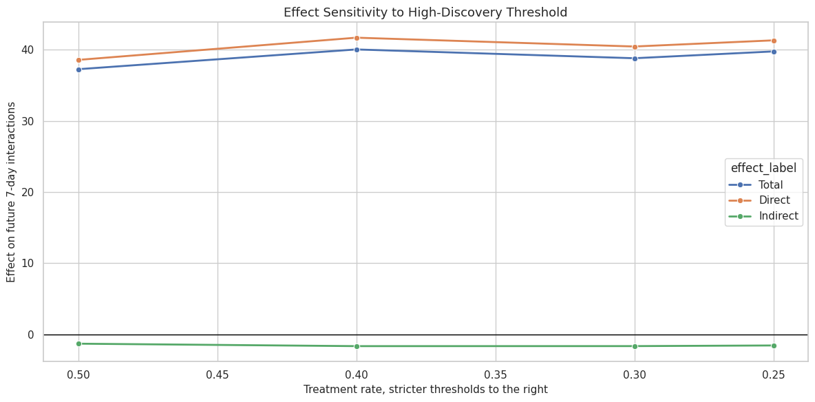
The threshold plot is a stability check. A jagged pattern would suggest that the result depends heavily on an arbitrary threshold. A smooth pattern is more reassuring.
8. Robustness to Alternative Mediator Definitions
The baseline mediator is a composite satisfaction-depth score. This cell reruns the mediation decomposition with simpler mediator candidates. The purpose is to test whether the indirect pathway is a property of satisfaction broadly or only of one engineered score.
mediator_rows = []
for mediator_label, mediator_col in mediator_candidates.items():
    result = estimate_binary_mediation_spec(
        analysis_panel,
        treatment_col=BASE_TREATMENT,
        mediator_col=mediator_col,
        outcome_col=PRIMARY_OUTCOME,
        numeric_cols=rich_numeric_covariates,
        categorical_cols=rich_categorical_covariates,
        spec_name=mediator_label,
        use_weights=True,
        include_interaction=True,
    )
    result["mediator_label"] = mediator_label
    mediator_rows.append(result)

mediator_results = pd.DataFrame(mediator_rows)

display(
    mediator_results[
        [
            "mediator_label",
            "mediator_col",
            "gcomp_total_effect",
            "natural_direct_effect",
            "natural_indirect_effect",
            "mediator_shift",
            "proportion_mediated",
            "mediator_model_r2",
        ]
    ].round(4)
)| mediator_label | mediator_col | gcomp_total_effect | natural_direct_effect | natural_indirect_effect | mediator_shift | proportion_mediated | mediator_model_r2 | |
|---|---|---|---|---|---|---|---|---|
| 0 | composite_satisfaction_depth | M_satisfaction_depth | 37.2781 | 38.5858 | -1.3077 | 0.0231 | -0.0351 | 0.4653 |
| 1 | high_watch_ratio_share | high_satisfaction_share | 37.2755 | 38.9900 | -1.7145 | 0.0424 | -0.0460 | 0.4301 |
| 2 | valid_play_share | valid_play_share | 37.3502 | 37.2221 | 0.1281 | 0.0065 | 0.0034 | 0.5762 |
| 3 | average_satisfaction_score | avg_satisfaction_score | 37.2560 | 38.5948 | -1.3388 | 0.0174 | -0.0359 | 0.4418 |
| 4 | completion_or_rewatch_share | complete_or_rewatch_share | 37.2665 | 38.7399 | -1.4734 | 0.0289 | -0.0395 | 0.4126 |
This is one of the most important checks. If all satisfaction mediators show small mediated pathways, the notebook 04 conclusion is more stable. If one mediator dominates, the final report should be precise about which satisfaction definition matters.
9. Plot Mediator Sensitivity
This cell plots the direct and indirect estimates across mediator definitions. It keeps the total effect visible as a reference but focuses attention on the mediated pathway.
mediator_plot = mediator_results.melt(
    id_vars=["mediator_label"],
    value_vars=["gcomp_total_effect", "natural_direct_effect", "natural_indirect_effect"],
    var_name="effect_type",
    value_name="estimate",
)
mediator_plot["effect_label"] = mediator_plot["effect_type"].map(
    {
        "gcomp_total_effect": "Total",
        "natural_direct_effect": "Direct",
        "natural_indirect_effect": "Indirect",
    }
)
mediator_plot["mediator_label_clean"] = mediator_plot["mediator_label"].str.replace("_", " ").str.title()

fig, ax = plt.subplots(figsize=(13, 6))
sns.barplot(
    data=mediator_plot,
    x="estimate",
    y="mediator_label_clean",
    hue="effect_label",
    ax=ax,
)
ax.axvline(0, color="black", linewidth=1)
ax.set_title("Effect Decomposition Across Mediator Definitions")
ax.set_xlabel("Effect on future 7-day interactions")
ax.set_ylabel("Mediator definition")
plt.tight_layout()
fig.savefig(FIGURE_DIR / "18_mediator_sensitivity.png", dpi=160, bbox_inches="tight")
plt.show()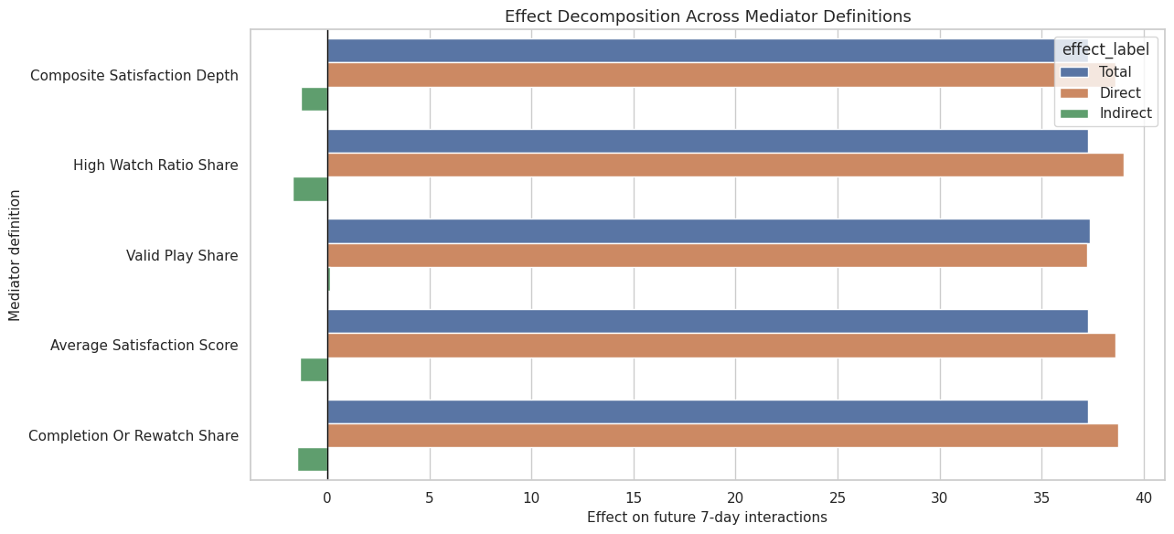
The mediator plot makes the main sensitivity question visible. A consistent direct-effect bar with small indirect bars supports the idea that future interaction gains are not mainly routed through these satisfaction proxies.
10. Robustness Across Outcomes
This cell repeats the baseline decomposition for future interactions, future active days, and future play hours. Notebook 04 already estimated these with bootstrap intervals; here we keep the point-estimate grid alongside the other robustness checks.
outcome_rows = []
for outcome_col in OUTCOME_COLUMNS:
    result = estimate_binary_mediation_spec(
        analysis_panel,
        treatment_col=BASE_TREATMENT,
        mediator_col=BASE_MEDIATOR,
        outcome_col=outcome_col,
        numeric_cols=rich_numeric_covariates,
        categorical_cols=rich_categorical_covariates,
        spec_name=f"baseline_{outcome_col}",
        use_weights=True,
        include_interaction=True,
    )
    outcome_rows.append(result)

outcome_results = pd.DataFrame(outcome_rows)

display(
    outcome_results[
        [
            "outcome_label",
            "gcomp_total_effect",
            "natural_direct_effect",
            "natural_indirect_effect",
            "mediator_shift",
            "relative_total_effect",
            "proportion_mediated",
        ]
    ].round(4)
)| outcome_label | gcomp_total_effect | natural_direct_effect | natural_indirect_effect | mediator_shift | relative_total_effect | proportion_mediated | |
|---|---|---|---|---|---|---|---|
| 0 | Future 7-day interactions | 37.2781 | 38.5858 | -1.3077 | 0.0231 | 0.1152 | -0.0351 |
| 1 | Future 7-day active days | 0.0074 | 0.0021 | 0.0053 | 0.0231 | 0.0011 | 0.7175 |
| 2 | Future 7-day play hours | 0.0784 | 0.0739 | 0.0044 | 0.0231 | 0.1000 | 0.0562 |
Different outcomes answer different product questions. Future interactions measure volume, active days measure return frequency, and play hours measure attention. A result can be meaningful for one and weak for another.
11. Sensitivity to Model Choices
This cell changes the model specification while holding the baseline treatment, mediator, and primary outcome fixed. It compares weighted versus unweighted regression, interaction versus no interaction, and rich versus simple controls.
model_specs = [
    {
        "spec_name": "weighted_rich_with_interaction",
        "use_weights": True,
        "include_interaction": True,
        "numeric_cols": rich_numeric_covariates,
        "categorical_cols": rich_categorical_covariates,
    },
    {
        "spec_name": "unweighted_rich_with_interaction",
        "use_weights": False,
        "include_interaction": True,
        "numeric_cols": rich_numeric_covariates,
        "categorical_cols": rich_categorical_covariates,
    },
    {
        "spec_name": "weighted_rich_no_interaction",
        "use_weights": True,
        "include_interaction": False,
        "numeric_cols": rich_numeric_covariates,
        "categorical_cols": rich_categorical_covariates,
    },
    {
        "spec_name": "weighted_simple_with_interaction",
        "use_weights": True,
        "include_interaction": True,
        "numeric_cols": simple_numeric_covariates,
        "categorical_cols": simple_categorical_covariates,
    },
    {
        "spec_name": "unweighted_simple_no_interaction",
        "use_weights": False,
        "include_interaction": False,
        "numeric_cols": simple_numeric_covariates,
        "categorical_cols": simple_categorical_covariates,
    },
]

model_rows = []
for spec in model_specs:
    result = estimate_binary_mediation_spec(
        analysis_panel,
        treatment_col=BASE_TREATMENT,
        mediator_col=BASE_MEDIATOR,
        outcome_col=PRIMARY_OUTCOME,
        numeric_cols=spec["numeric_cols"],
        categorical_cols=spec["categorical_cols"],
        spec_name=spec["spec_name"],
        use_weights=spec["use_weights"],
        include_interaction=spec["include_interaction"],
    )
    result["control_set"] = "rich" if len(spec["numeric_cols"]) == len(rich_numeric_covariates) else "simple"
    model_rows.append(result)

model_sensitivity = pd.DataFrame(model_rows)

display(
    model_sensitivity[
        [
            "spec_name",
            "uses_weights",
            "include_interaction",
            "control_set",
            "gcomp_total_effect",
            "natural_direct_effect",
            "natural_indirect_effect",
            "mediator_shift",
            "relative_total_effect",
        ]
    ].round(4)
)| spec_name | uses_weights | include_interaction | control_set | gcomp_total_effect | natural_direct_effect | natural_indirect_effect | mediator_shift | relative_total_effect | |
|---|---|---|---|---|---|---|---|---|---|
| 0 | weighted_rich_with_interaction | True | True | rich | 37.2781 | 38.5858 | -1.3077 | 0.0231 | 0.1152 |
| 1 | unweighted_rich_with_interaction | False | True | rich | 36.4288 | 37.9141 | -1.4853 | 0.0229 | 0.1130 |
| 2 | weighted_rich_no_interaction | True | False | rich | 37.3139 | 38.4311 | -1.1172 | 0.0231 | 0.1153 |
| 3 | weighted_simple_with_interaction | True | True | simple | 37.6289 | 39.1871 | -1.5581 | 0.0347 | 0.1169 |
| 4 | unweighted_simple_no_interaction | False | False | simple | 34.8085 | 35.7445 | -0.9360 | 0.0320 | 0.1077 |
This table tells us whether the result is mostly a modeling artifact. A stable total effect across these rows is reassuring. A highly variable indirect effect would tell us to be cautious about strong claims about the mediator pathway.
12. Plot Model-Specification Sensitivity
This cell visualizes the model-sensitivity table. It keeps direct and indirect pieces side by side for each model choice.
model_plot = model_sensitivity.melt(
    id_vars=["spec_name"],
    value_vars=["gcomp_total_effect", "natural_direct_effect", "natural_indirect_effect"],
    var_name="effect_type",
    value_name="estimate",
)
model_plot["effect_label"] = model_plot["effect_type"].map(
    {
        "gcomp_total_effect": "Total",
        "natural_direct_effect": "Direct",
        "natural_indirect_effect": "Indirect",
    }
)
model_plot["spec_label"] = model_plot["spec_name"].str.replace("_", " ").str.title()

fig, ax = plt.subplots(figsize=(13, 7))
sns.barplot(
    data=model_plot,
    x="estimate",
    y="spec_label",
    hue="effect_label",
    ax=ax,
)
ax.axvline(0, color="black", linewidth=1)
ax.set_title("Effect Decomposition Across Model Choices")
ax.set_xlabel("Effect on future 7-day interactions")
ax.set_ylabel("Model choice")
plt.tight_layout()
fig.savefig(FIGURE_DIR / "19_model_sensitivity.png", dpi=160, bbox_inches="tight")
plt.show()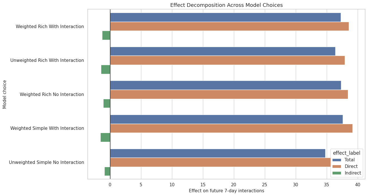
The model-sensitivity plot is a compact way to see which part of the story is stable. In a strong result, the total effect should not depend on one narrow modeling choice.
13. Continuous Discovery Score Check
The binary treatment is easy to explain, but it loses information. This cell treats discovery_breadth_score as continuous and estimates adjusted associations per 0.10 increase in discovery breadth. This is not a natural-effect decomposition; it is a separate dose-style sensitivity check.
def estimate_continuous_association(frame, score_col, target_col, numeric_cols, categorical_cols, scale=0.10):
    covariates = build_covariate_matrix(frame, numeric_cols, categorical_cols)
    score = frame[score_col].astype(float).to_numpy()
    target = frame[target_col].astype(float).to_numpy()
    design = covariates.copy()
    design.insert(0, score_col, score)
    model = LinearRegression().fit(design, target)
    coef = float(model.coef_[0])
    return {
        "target": target_col,
        "target_label": OUTCOME_LABELS.get(target_col, target_col),
        "score_col": score_col,
        "effect_per_0_10_score_increase": coef * scale,
        "raw_score_target_corr": frame[score_col].corr(frame[target_col], method="spearman"),
        "model_r2": model.score(design, target),
    }

continuous_rows = []
for target_col in OUTCOME_COLUMNS + [BASE_MEDIATOR]:
    continuous_rows.append(
        estimate_continuous_association(
            analysis_panel,
            DISCOVERY_SCORE,
            target_col,
            rich_numeric_covariates,
            rich_categorical_covariates,
        )
    )
continuous_sensitivity = pd.DataFrame(continuous_rows)

display(continuous_sensitivity.round(4))| target | target_label | score_col | effect_per_0_10_score_increase | raw_score_target_corr | model_r2 | |
|---|---|---|---|---|---|---|
| 0 | Y_future_interactions | Future 7-day interactions | discovery_breadth_score | 20.5518 | 0.5674 | 0.7220 |
| 1 | Y_future_active_days | Future 7-day active days | discovery_breadth_score | 0.0966 | 0.3980 | 0.5179 |
| 2 | Y_future_play_hours | Future 7-day play hours | discovery_breadth_score | 0.0447 | 0.5392 | 0.6999 |
| 3 | M_satisfaction_depth | M_satisfaction_depth | discovery_breadth_score | 0.0129 | 0.0930 | 0.4612 |
The continuous check asks whether more discovery breadth is associated with more future value without forcing a high-versus-low split. It should broadly agree with the binary result if the threshold is not doing all the work.
14. Placebo-Style Checks for Pre-Period Activity and Calendar Time
A dangerous pattern would be high discovery exposure strongly predicting variables that happened before the treatment day. This cell checks raw and adjusted relationships between high discovery and pre-period activity, prior satisfaction, prior discovery, and calendar day.
placebo_targets = [
    "lag_1_interactions",
    "prior_3day_interactions",
    "prior_3day_high_satisfaction_share",
    "prior_3day_discovery_candidate_share",
    "calendar_day_index",
]

placebo_adjustment_numeric = [
    col
    for col in ["register_days", "follow_user_num", "fans_user_num", "friend_user_num", "is_lowactive_period", "is_live_streamer", "is_video_author"]
    if col in analysis_panel.columns
] + profile_onehot_covariates
placebo_adjustment_categorical = rich_categorical_covariates

placebo_rows = []
for target_col in placebo_targets:
    raw_high = analysis_panel.loc[analysis_panel[BASE_TREATMENT].eq(1), target_col].mean()
    raw_low = analysis_panel.loc[analysis_panel[BASE_TREATMENT].eq(0), target_col].mean()

    numeric_cols = [col for col in placebo_adjustment_numeric if col != target_col]
    categorical_cols = [col for col in placebo_adjustment_categorical if col != target_col]
    covariates = build_covariate_matrix(analysis_panel, numeric_cols, categorical_cols)
    design = covariates.copy()
    design.insert(0, BASE_TREATMENT, analysis_panel[BASE_TREATMENT].astype(float).to_numpy())
    model = LinearRegression().fit(design, analysis_panel[target_col].astype(float).to_numpy())
    adjusted_difference = float(model.coef_[0])

    placebo_rows.append(
        {
            "placebo_target": target_col,
            "raw_high_minus_lower": raw_high - raw_low,
            "adjusted_difference": adjusted_difference,
            "target_mean": analysis_panel[target_col].mean(),
            "relative_raw_difference": (raw_high - raw_low) / analysis_panel[target_col].mean() if not np.isclose(analysis_panel[target_col].mean(), 0) else np.nan,
        }
    )

placebo_checks = pd.DataFrame(placebo_rows)

display(placebo_checks.round(4))| placebo_target | raw_high_minus_lower | adjusted_difference | target_mean | relative_raw_difference | |
|---|---|---|---|---|---|
| 0 | lag_1_interactions | 18.3176 | 18.3670 | 51.0316 | 0.3589 |
| 1 | prior_3day_interactions | 49.0163 | 49.1383 | 152.5819 | 0.3212 |
| 2 | prior_3day_high_satisfaction_share | -0.0321 | -0.0363 | 1.3416 | -0.0239 |
| 3 | prior_3day_discovery_candidate_share | 0.3502 | 0.3493 | 1.0706 | 0.3271 |
| 4 | calendar_day_index | -15.6133 | -15.6544 | 30.7969 | -0.5070 |
The placebo-style checks are expected to show some pre-period differences because discovery exposure is not randomized. The point is to make that imbalance visible and connect it back to the need for adjustment and sensitivity analysis.
15. Plot Placebo-Style Checks
This cell plots raw and adjusted pre-period differences. Large pre-period differences are not fatal by themselves, but they are a warning against overclaiming from observational logs.
placebo_plot = placebo_checks.melt(
    id_vars=["placebo_target"],
    value_vars=["raw_high_minus_lower", "adjusted_difference"],
    var_name="contrast_type",
    value_name="difference",
)
placebo_plot["contrast_type"] = placebo_plot["contrast_type"].map(
    {
        "raw_high_minus_lower": "Raw high - lower",
        "adjusted_difference": "Adjusted difference",
    }
)
placebo_plot["target_label"] = placebo_plot["placebo_target"].str.replace("_", " ").str.title()

fig, ax = plt.subplots(figsize=(12, 6))
sns.barplot(data=placebo_plot, x="difference", y="target_label", hue="contrast_type", ax=ax)
ax.axvline(0, color="black", linewidth=1)
ax.set_title("Placebo-Style Checks on Pre-Period Variables")
ax.set_xlabel("High-discovery minus lower-discovery difference")
ax.set_ylabel("Pre-period or calendar variable")
plt.tight_layout()
fig.savefig(FIGURE_DIR / "20_placebo_preperiod_checks.png", dpi=160, bbox_inches="tight")
plt.show()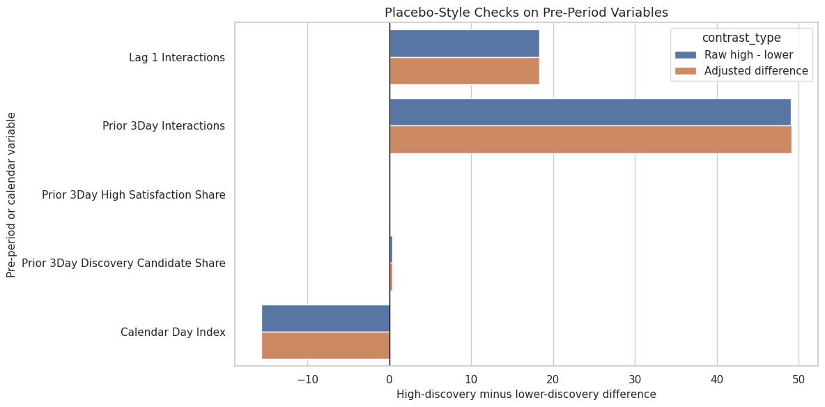
This plot helps communicate why the earlier balance and propensity diagnostics matter. The treatment is observational, so a final report should emphasize adjusted estimates and limitations rather than raw gaps.
16. Summarize Robustness Patterns
This cell creates a compact summary across robustness families. It focuses on whether the total effect stays positive and whether the indirect effect remains small relative to the direct effect.
robustness_families = []

for family_name, frame in [
    ("threshold_sensitivity", threshold_results),
    ("mediator_sensitivity", mediator_results),
    ("model_sensitivity", model_sensitivity),
    ("outcome_sensitivity", outcome_results.query("outcome == @PRIMARY_OUTCOME")),
]:
    robustness_families.append(
        {
            "robustness_family": family_name,
            "specifications": len(frame),
            "total_effect_min": frame["gcomp_total_effect"].min(),
            "total_effect_max": frame["gcomp_total_effect"].max(),
            "total_effect_share_positive": (frame["gcomp_total_effect"] > 0).mean(),
            "indirect_effect_min": frame["natural_indirect_effect"].min(),
            "indirect_effect_max": frame["natural_indirect_effect"].max(),
            "indirect_effect_share_positive": (frame["natural_indirect_effect"] > 0).mean(),
            "median_abs_indirect_to_total_ratio": np.nanmedian(
                np.abs(frame["natural_indirect_effect"] / frame["gcomp_total_effect"].replace(0, np.nan))
            ),
        }
    )

robustness_summary = pd.DataFrame(robustness_families)

display(robustness_summary.round(4))| robustness_family | specifications | total_effect_min | total_effect_max | total_effect_share_positive | indirect_effect_min | indirect_effect_max | indirect_effect_share_positive | median_abs_indirect_to_total_ratio | |
|---|---|---|---|---|---|---|---|---|---|
| 0 | threshold_sensitivity | 4 | 37.2781 | 40.0555 | 1.0 | -1.6532 | -1.3077 | 0.0 | 0.0402 |
| 1 | mediator_sensitivity | 5 | 37.2560 | 37.3502 | 1.0 | -1.7145 | 0.1281 | 0.2 | 0.0359 |
| 2 | model_sensitivity | 5 | 34.8085 | 37.6289 | 1.0 | -1.5581 | -0.9360 | 0.0 | 0.0351 |
| 3 | outcome_sensitivity | 1 | 37.2781 | 37.2781 | 1.0 | -1.3077 | -1.3077 | 0.0 | 0.0351 |
This summary turns many model runs into a few takeaways. The strongest claim is the one that remains stable across robustness families. The weaker claim is the one that moves around or depends on a specific metric definition.
17. Limitations Table
This cell writes a limitations table for the final report. These are not flaws to hide. They are the boundaries that make the analysis honest and more believable.
limitations = pd.DataFrame(
    [
        {
            "limitation": "observational_recommendation_logs",
            "why_it_matters": "High-discovery exposure was not randomized, so user preferences and recommender selection can confound estimates.",
            "mitigation_in_this_work": "Used pre-treatment history/profile controls, propensity diagnostics, and weighted sensitivity checks.",
            "remaining_risk": "Unobserved ranking-system state and user intent can still bias estimates.",
        },
        {
            "limitation": "mediator_outcome_confounding",
            "why_it_matters": "Satisfaction depth and future engagement may share unobserved causes.",
            "mitigation_in_this_work": "Checked residual mediator-outcome relationships and compared multiple mediator definitions.",
            "remaining_risk": "Natural direct and indirect effects rely on strong mediator assumptions.",
        },
        {
            "limitation": "satisfaction_proxy_measurement",
            "why_it_matters": "Watch ratio and valid play are proxies, not direct surveys of satisfaction.",
            "mitigation_in_this_work": "Compared composite satisfaction, high watch ratio, valid play, average score, and completion-style mediators.",
            "remaining_risk": "The chosen proxies may miss frustration, novelty value, or long-run satisfaction.",
        },
        {
            "limitation": "active_day_sample_selection",
            "why_it_matters": "The analysis conditions on active user-days, so it does not study days with no observed interactions.",
            "mitigation_in_this_work": "Defined the estimand clearly for active days and reported active-day alternate outcomes.",
            "remaining_risk": "Results may not generalize to dormant users or cold-start retention decisions.",
        },
        {
            "limitation": "calendar_and_history_imbalance",
            "why_it_matters": "High discovery days differ from lower discovery days in time and recent behavior.",
            "mitigation_in_this_work": "Included calendar/history controls and showed placebo-style pre-period checks.",
            "remaining_risk": "Residual time-varying confounding can remain after observed adjustment.",
        },
    ]
)

display(limitations)| limitation | why_it_matters | mitigation_in_this_work | remaining_risk | |
|---|---|---|---|---|
| 0 | observational_recommendation_logs | High-discovery exposure was not randomized, so user preferences and recommender selection can confound estimates. | Used pre-treatment history/profile controls, propensity diagnostics, and weighted sensitivity checks. | Unobserved ranking-system state and user intent can still bias estimates. |
| 1 | mediator_outcome_confounding | Satisfaction depth and future engagement may share unobserved causes. | Checked residual mediator-outcome relationships and compared multiple mediator definitions. | Natural direct and indirect effects rely on strong mediator assumptions. |
| 2 | satisfaction_proxy_measurement | Watch ratio and valid play are proxies, not direct surveys of satisfaction. | Compared composite satisfaction, high watch ratio, valid play, average score, and completion-style mediators. | The chosen proxies may miss frustration, novelty value, or long-run satisfaction. |
| 3 | active_day_sample_selection | The analysis conditions on active user-days, so it does not study days with no observed interactions. | Defined the estimand clearly for active days and reported active-day alternate outcomes. | Results may not generalize to dormant users or cold-start retention decisions. |
| 4 | calendar_and_history_imbalance | High discovery days differ from lower discovery days in time and recent behavior. | Included calendar/history controls and showed placebo-style pre-period checks. | Residual time-varying confounding can remain after observed adjustment. |
The limitations table gives the final report a professional tone. It shows that the analysis is careful about where the evidence is strong and where it remains assumption-dependent.
18. Save Robustness Outputs
This cell saves all robustness tables to data/processed and mirrors the main tables into the notebook writeup folder.
threshold_results.to_csv(THRESHOLD_OUTPUT, index=False)
mediator_results.to_csv(MEDIATOR_OUTPUT, index=False)
model_sensitivity.to_csv(MODEL_SENSITIVITY_OUTPUT, index=False)
continuous_sensitivity.to_csv(CONTINUOUS_OUTPUT, index=False)
placebo_checks.to_csv(PLACEBO_OUTPUT, index=False)
robustness_summary.to_csv(ROBUSTNESS_SUMMARY_OUTPUT, index=False)
limitations.to_csv(LIMITATIONS_OUTPUT, index=False)

threshold_results.to_csv(TABLE_DIR / "robustness_thresholds.csv", index=False)
mediator_results.to_csv(TABLE_DIR / "robustness_mediators.csv", index=False)
model_sensitivity.to_csv(TABLE_DIR / "model_sensitivity.csv", index=False)
continuous_sensitivity.to_csv(TABLE_DIR / "continuous_score_sensitivity.csv", index=False)
placebo_checks.to_csv(TABLE_DIR / "placebo_checks.csv", index=False)
robustness_summary.to_csv(TABLE_DIR / "robustness_summary.csv", index=False)
limitations.to_csv(TABLE_DIR / "limitations.csv", index=False)

saved_outputs = pd.DataFrame(
    {
        "artifact": [
            "threshold_robustness",
            "mediator_robustness",
            "model_sensitivity",
            "continuous_score_sensitivity",
            "placebo_checks",
            "robustness_summary",
            "limitations",
        ],
        "path": [
            str(THRESHOLD_OUTPUT),
            str(MEDIATOR_OUTPUT),
            str(MODEL_SENSITIVITY_OUTPUT),
            str(CONTINUOUS_OUTPUT),
            str(PLACEBO_OUTPUT),
            str(ROBUSTNESS_SUMMARY_OUTPUT),
            str(LIMITATIONS_OUTPUT),
        ],
    }
)

display(saved_outputs)| artifact | path | |
|---|---|---|
| 0 | threshold_robustness | /home/apex/Documents/ranking_sys/data/processed/kuairec_discovery_quality_robustness_thresholds.csv |
| 1 | mediator_robustness | /home/apex/Documents/ranking_sys/data/processed/kuairec_discovery_quality_robustness_mediators.csv |
| 2 | model_sensitivity | /home/apex/Documents/ranking_sys/data/processed/kuairec_discovery_quality_model_sensitivity.csv |
| 3 | continuous_score_sensitivity | /home/apex/Documents/ranking_sys/data/processed/kuairec_discovery_quality_continuous_score_sensitivity.csv |
| 4 | placebo_checks | /home/apex/Documents/ranking_sys/data/processed/kuairec_discovery_quality_placebo_checks.csv |
| 5 | robustness_summary | /home/apex/Documents/ranking_sys/data/processed/kuairec_discovery_quality_robustness_summary.csv |
| 6 | limitations | /home/apex/Documents/ranking_sys/data/processed/kuairec_discovery_quality_limitations.csv |
The saved outputs make this robustness work reusable. A final report can pull directly from these tables without recomputing the sensitivity grid.
19. Notebook Takeaways
This notebook stress-tested the mediation result from several angles:
- The total future-interaction effect is checked across stricter discovery thresholds.
- The mediated pathway is checked across several satisfaction proxy definitions.
- The result is compared across future interactions, active days, and play hours.
- Model choices are varied through weighting, interactions, and control-set size.
- Placebo-style checks make pre-period imbalance visible.
- The limitations table records what the observational design cannot fully solve.
The next notebook should be the final report and figures notebook for this discovery-quality mediation project. It should turn the evidence into a concise portfolio-ready narrative with the key tables, plots, and caveats.