Direct, Indirect, and Total Effects for Discovery Quality

The previous notebook defined the mediation design. This notebook estimates the effects.

The causal story is built around three variables:

• A_high_discovery: whether an active user-day had high discovery breadth.
• M_satisfaction_depth: same-day satisfaction depth, built from watch-quality signals.
• Y: future user value, primarily future seven-day interactions.

The goal is to decompose the effect of high discovery exposure into:

• Total effect: the overall adjusted difference in future value between high-discovery and lower-discovery days.
• Natural direct effect: the part of the difference that remains if satisfaction depth is held at the lower-discovery counterfactual level.
• Natural indirect effect: the part of the difference that flows through the change in satisfaction depth.
• Controlled direct effects: treatment contrasts at fixed low, median, and high satisfaction levels.

This is still an observational analysis, so the estimates should be read as adjusted causal estimates under the assumptions documented in notebook 03. The notebook uses g-computation because it makes the counterfactual logic visible and easy to explain.

1. Load Libraries and Paths

This cell imports the modeling, plotting, and utility libraries used in the notebook. The path logic works from either the repository root or the notebook folder, which keeps the notebook portable across VS Code and Jupyter sessions.

from pathlib import Path
import warnings
import os

os.environ.setdefault("OMP_NUM_THREADS", "1")
os.environ.setdefault("OPENBLAS_NUM_THREADS", "1")
os.environ.setdefault("MKL_NUM_THREADS", "1")
os.environ.setdefault("NUMEXPR_NUM_THREADS", "1")

import numpy as np
import pandas as pd
import seaborn as sns
import matplotlib.pyplot as plt
from IPython.display import display
from sklearn.linear_model import LinearRegression

warnings.filterwarnings("ignore", category=FutureWarning)

sns.set_theme(style="whitegrid", context="notebook")
plt.rcParams["figure.figsize"] = (11, 6)
plt.rcParams["axes.titlesize"] = 13
plt.rcParams["axes.labelsize"] = 11
pd.set_option("display.max_columns", 160)
pd.set_option("display.max_colwidth", 140)

PROJECT_ROOT = Path.cwd().resolve()
while not (PROJECT_ROOT / "data").exists() and PROJECT_ROOT.parent != PROJECT_ROOT:
    PROJECT_ROOT = PROJECT_ROOT.parent

PROCESSED_DIR = PROJECT_ROOT / "data" / "processed"
NOTEBOOK_DIR = PROJECT_ROOT / "notebooks" / "discovery_quality_mediation"
WRITEUP_DIR = NOTEBOOK_DIR / "writeup"
FIGURE_DIR = WRITEUP_DIR / "figures"
TABLE_DIR = WRITEUP_DIR / "tables"

FIGURE_DIR.mkdir(parents=True, exist_ok=True)
TABLE_DIR.mkdir(parents=True, exist_ok=True)

ANALYSIS_PANEL_INPUT = PROCESSED_DIR / "kuairec_discovery_quality_mediation_analysis_panel.parquet"
ESTIMAND_REGISTRY_INPUT = PROCESSED_DIR / "kuairec_discovery_quality_estimand_registry.csv"
ASSUMPTION_CHECKS_INPUT = PROCESSED_DIR / "kuairec_discovery_quality_assumption_checks.csv"
MODEL_BLUEPRINT_INPUT = PROCESSED_DIR / "kuairec_discovery_quality_mediation_model_blueprint.csv"

EFFECT_ESTIMATES_OUTPUT = PROCESSED_DIR / "kuairec_discovery_quality_effect_estimates.csv"
BOOTSTRAP_EFFECTS_OUTPUT = PROCESSED_DIR / "kuairec_discovery_quality_bootstrap_effects.csv"
EFFECT_SUMMARY_OUTPUT = PROCESSED_DIR / "kuairec_discovery_quality_effect_summary.csv"
CONTROLLED_DIRECT_OUTPUT = PROCESSED_DIR / "kuairec_discovery_quality_controlled_direct_effects.csv"
MODEL_DIAGNOSTICS_OUTPUT = PROCESSED_DIR / "kuairec_discovery_quality_effect_model_diagnostics.csv"

The notebook writes both machine-readable outputs in data/processed and writeup-friendly copies in notebooks/projects/project_5_discovery_quality_mediation/writeup/tables. That way the next notebooks and final report can reuse the exact same estimates.

2. Load the Mediation Analysis Panel

This cell loads the panel saved by notebook 03, along with the estimand and assumption tables. The panel already contains the treatment, mediator, outcomes, propensity scores, and capped stabilized weights needed for adjusted estimation.

analysis_panel = pd.read_parquet(ANALYSIS_PANEL_INPUT)
estimand_registry = pd.read_csv(ESTIMAND_REGISTRY_INPUT)
assumption_checks = pd.read_csv(ASSUMPTION_CHECKS_INPUT)
model_blueprint = pd.read_csv(MODEL_BLUEPRINT_INPUT)

load_summary = pd.DataFrame(
    {
        "artifact": ["analysis_panel", "estimand_registry", "assumption_checks", "model_blueprint"],
        "rows": [len(analysis_panel), len(estimand_registry), len(assumption_checks), len(model_blueprint)],
        "columns": [analysis_panel.shape[1], estimand_registry.shape[1], assumption_checks.shape[1], model_blueprint.shape[1]],
    }
)

display(load_summary)
display(analysis_panel[["user_id", "event_date", "A_high_discovery", "M_satisfaction_depth", "Y_future_interactions"]].head())

	artifact	rows	columns
0	analysis_panel	8199	103
1	estimand_registry	5	5
2	assumption_checks	6	5
3	model_blueprint	5	4

	user_id	event_date	A_high_discovery	M_satisfaction_depth	Y_future_interactions
0	120	2020-07-05	1	0.469690	316.0
1	120	2020-07-06	1	0.549183	345.0
2	120	2020-07-07	1	0.501650	393.0
3	120	2020-07-08	1	0.444413	436.0
4	120	2020-07-09	0	0.570206	448.0

The loaded panel is already at the correct analysis grain: one active user-day per row. That matters because treatment, mediator, and future outcomes all refer to the same user-day timeline.

3. Reconfirm the Estimands and Assumptions

This cell displays the design commitments from notebook 03. This is not just documentation. It reminds us that the estimates below are only meaningful under the assumptions listed here, especially observed adjustment, overlap, and sensitivity to unobserved mediator-outcome confounding.

display(estimand_registry)
display(assumption_checks)
display(model_blueprint)

	estimand	symbol	definition	plain_language	answers
0	total_effect	TE	E[Y(1, M(1)) - Y(0, M(0))]	Overall difference in future value between high-discovery and lower-discovery days.	Does high discovery exposure relate to future value at all?
1	natural_direct_effect	NDE	E[Y(1, M(0)) - Y(0, M(0))]	Effect of high discovery exposure while holding the mediator at its lower-discovery counterfactual level.	How much of the effect bypasses satisfaction depth?
2	natural_indirect_effect	NIE	E[Y(1, M(1)) - Y(1, M(0))]	Effect transmitted through the change in satisfaction depth caused by high discovery exposure.	How much of the effect flows through satisfaction?
3	controlled_direct_effect_low_mediator	CDE_low	E[Y(1, m_low) - Y(0, m_low)]	Direct treatment contrast if satisfaction depth were fixed to a low reference value.	What is the direct exposure effect under weak satisfaction?
4	controlled_direct_effect_high_mediator	CDE_high	E[Y(1, m_high) - Y(0, m_high)]	Direct treatment contrast if satisfaction depth were fixed to a high reference value.	What is the direct exposure effect under strong satisfaction?

	assumption	status	diagnostic	value	risk_if_violated
0	consistency	design_definition	Treatment, mediator, and outcome are defined at the user-day level with no future information in A or M.	A=high discovery day; M=satisfaction depth; Y=future 7-day interactions	Effects would mix incompatible versions of discovery exposure.
1	positivity_overlap	checked	Propensity score support and extreme propensity shares.	p05=0.042, p95=0.860	Estimates would rely on extrapolating to user-days with little comparable data.
2	observed_treatment_exchangeability	partially_checked	Numeric covariate balance before and after capped stabilized weighting.	max weighted abs SMD=0.157	The high-discovery contrast could reflect user history rather than exposure.
3	observed_mediator_outcome_adjustment	partially_checked	Residual mediator-outcome relationship after observed covariates.	residual Spearman=-0.019	The indirect pathway could be confounded by unmeasured user intent or recommendation state.
4	no_unmeasured_confounding	not_testable	Requires domain argument and sensitivity analysis.	Not guaranteed by observational KuaiRec logs.	Direct and indirect effects may not support a causal reading.
5	no_treatment_induced_mediator_outcome_confounder	not_testable	Requires design argument; avoid adjusting for post-treatment variables affected by A.	Use pre-treatment history/profile controls in primary setup.	Mediation decomposition can be biased even if treatment and mediator models fit well.

	model_step	target	formula_concept	purpose
0	total_effect_model	Y_future_interactions	Y ~ A + X	Estimate the overall association of high discovery exposure with future value after observed adjustment.
1	mediator_model	M_satisfaction_depth	M ~ A + X	Estimate how high discovery exposure shifts satisfaction depth after observed adjustment.
2	outcome_mediation_model	Y_future_interactions	Y ~ A + M + A*M + X	Estimate how treatment and mediator jointly predict future value after observed adjustment.
3	counterfactual_prediction	Y(a, M(a_prime))	Predict mediator under A=0/1, then predict outcome under treatment-mediator combinations.	Compute total, natural direct, natural indirect, and controlled direct effects by averaging predictions.
4	bootstrap_uncertainty	effect intervals	Resample users, not rows, to respect repeated user-days.	Quantify uncertainty while acknowledging clustered user-day observations.

The estimand table is the contract for the notebook. The code below estimates the quantities in that table rather than treating a single regression coefficient as the whole answer.

4. Define Outcomes, Controls, and Analysis Settings

This cell defines the primary outcome, alternate outcomes, covariates, and bootstrap settings. The covariate set mirrors notebook 03: pre-treatment history, calendar time, user profile signals, and static encoded features.

TREATMENT = "A_high_discovery"
MEDIATOR = "M_satisfaction_depth"
PRIMARY_OUTCOME = "Y_future_interactions"
OUTCOME_COLUMNS = ["Y_future_interactions", "Y_future_active_days", "Y_future_play_hours"]
OUTCOME_LABELS = {
    "Y_future_interactions": "Future 7-day interactions",
    "Y_future_active_days": "Future 7-day active days",
    "Y_future_play_hours": "Future 7-day play hours",
}
WEIGHT_COLUMN = "stabilized_ipw_capped"
BOOTSTRAP_ITERATIONS = 75
RANDOM_SEED = 42

base_numeric_covariates = [
    "calendar_day_index",
    "lag_1_active_day",
    "prior_3day_active_day",
    "lag_1_interactions",
    "prior_3day_interactions",
    "lag_1_total_play_duration_sec",
    "prior_3day_total_play_duration_sec",
    "lag_1_valid_play_share",
    "prior_3day_valid_play_share",
    "lag_1_high_satisfaction_share",
    "prior_3day_high_satisfaction_share",
    "lag_1_discovery_candidate_share",
    "prior_3day_discovery_candidate_share",
    "recent_activity_score",
    "register_days",
    "follow_user_num",
    "fans_user_num",
    "friend_user_num",
    "is_lowactive_period",
    "is_live_streamer",
    "is_video_author",
]
profile_onehot_covariates = [col for col in analysis_panel.columns if col.startswith("onehot_feat")]
numeric_covariates = [col for col in base_numeric_covariates + profile_onehot_covariates if col in analysis_panel.columns]
categorical_covariates = [
    col
    for col in [
        "user_active_degree",
        "follow_user_num_range",
        "fans_user_num_range",
        "friend_user_num_range",
        "register_days_range",
    ]
    if col in analysis_panel.columns
]

settings_summary = pd.DataFrame(
    {
        "setting": [
            "treatment",
            "mediator",
            "primary_outcome",
            "alternate_outcomes",
            "numeric_covariates",
            "categorical_covariates",
            "bootstrap_iterations",
            "bootstrap_unit",
        ],
        "value": [
            TREATMENT,
            MEDIATOR,
            PRIMARY_OUTCOME,
            ", ".join([col for col in OUTCOME_COLUMNS if col != PRIMARY_OUTCOME]),
            len(numeric_covariates),
            len(categorical_covariates),
            BOOTSTRAP_ITERATIONS,
            "user_id",
        ],
    }
)

display(settings_summary)

	setting	value
0	treatment	A_high_discovery
1	mediator	M_satisfaction_depth
2	primary_outcome	Y_future_interactions
3	alternate_outcomes	Y_future_active_days, Y_future_play_hours
4	numeric_covariates	39
5	categorical_covariates	5
6	bootstrap_iterations	75
7	bootstrap_unit	user_id

The bootstrap unit is user_id, not row. Each user contributes multiple days, so resampling rows would make the uncertainty look too confident. User-level resampling keeps repeated observations together.

5. Prepare Helper Functions for G-Computation

This cell defines the core reusable functions. The key idea is simple:

1. Fit a mediator model: M ~ A + X.
2. Predict each user’s mediator under A=0 and A=1.
3. Fit an outcome model: Y ~ A + M + A*M + X.
4. Predict counterfactual outcomes under combinations like Y(1, M(0)) and Y(1, M(1)).

The functions keep the mechanics in one place so later cells can focus on results.

def build_covariate_matrix(frame, numeric_cols, categorical_cols):
    """Create a numeric model matrix from pre-treatment covariates."""
    numeric = frame[numeric_cols].copy()
    for col in numeric.columns:
        numeric[col] = pd.to_numeric(numeric[col], errors="coerce")
        numeric[col] = numeric[col].fillna(numeric[col].median())

    if categorical_cols:
        categorical = frame[categorical_cols].copy()
        for col in categorical.columns:
            categorical[col] = categorical[col].astype("string").fillna("missing")
        encoded = pd.get_dummies(categorical, drop_first=True, dtype=float)
        design = pd.concat([numeric, encoded], axis=1)
    else:
        design = numeric

    design = design.loc[:, design.nunique(dropna=False) > 1]
    return design.astype(float)


def treatment_design(covariates, treatment_values):
    """Create design matrix for models that use treatment and covariates."""
    design = covariates.copy()
    design.insert(0, TREATMENT, np.asarray(treatment_values, dtype=float))
    return design


def outcome_design(covariates, treatment_values, mediator_values):
    """Create design matrix for the outcome mediation model."""
    treatment_array = np.asarray(treatment_values, dtype=float)
    mediator_array = np.asarray(mediator_values, dtype=float)
    design = covariates.copy()
    design.insert(0, "A_x_M", treatment_array * mediator_array)
    design.insert(0, MEDIATOR, mediator_array)
    design.insert(0, TREATMENT, treatment_array)
    return design


def weighted_average(values, weights=None):
    """Average values with optional weights; use ordinary mean when weights are absent."""
    values = np.asarray(values, dtype=float)
    if weights is None:
        return float(np.mean(values))
    weights = np.asarray(weights, dtype=float)
    return float(np.average(values, weights=weights))


def fit_linear_model(X, y, sample_weight=None):
    """Fit a linear regression model with optional sample weights."""
    model = LinearRegression()
    model.fit(X, y, sample_weight=sample_weight)
    return model

helper_summary = pd.DataFrame(
    {
        "helper": ["build_covariate_matrix", "treatment_design", "outcome_design", "weighted_average", "fit_linear_model"],
        "purpose": [
            "Create the pre-treatment adjustment matrix.",
            "Build A + X matrices for total and mediator models.",
            "Build A + M + A*M + X matrices for outcome models.",
            "Average counterfactual predictions over the target population.",
            "Fit the linear models used for transparent g-computation.",
        ],
    }
)

display(helper_summary)

	helper	purpose
0	build_covariate_matrix	Create the pre-treatment adjustment matrix.
1	treatment_design	Build A + X matrices for total and mediator models.
2	outcome_design	Build A + M + A*M + X matrices for outcome models.
3	weighted_average	Average counterfactual predictions over the target population.
4	fit_linear_model	Fit the linear models used for transparent g-computation.

The helper functions use linear models because the goal is transparent decomposition. Later sensitivity notebooks can swap in flexible models, but this notebook prioritizes an understandable baseline.

6. Implement the Effect Estimator

This cell implements the actual g-computation estimator. It returns point estimates for raw differences, adjusted total effects, natural direct and indirect effects, and controlled direct effects. The same function is later reused inside the bootstrap loop.

def estimate_mediation_effects(frame, outcome_columns, use_weights=True):
    """Estimate mediation effects for one frame and one set of outcomes."""
    working = frame.copy().reset_index(drop=True)
    covariates = build_covariate_matrix(working, numeric_covariates, categorical_covariates)
    A_observed = working[TREATMENT].astype(float).to_numpy()
    M_observed = working[MEDIATOR].astype(float).to_numpy()
    weights = working[WEIGHT_COLUMN].astype(float).to_numpy() if use_weights and WEIGHT_COLUMN in working.columns else None
    averaging_weights = None

    # Mediator counterfactuals M(0) and M(1).
    mediator_X = treatment_design(covariates, A_observed)
    mediator_model = fit_linear_model(mediator_X, M_observed, sample_weight=weights)
    M0 = mediator_model.predict(treatment_design(covariates, np.zeros(len(working)))).clip(0, 1)
    M1 = mediator_model.predict(treatment_design(covariates, np.ones(len(working)))).clip(0, 1)
    mediator_shift = weighted_average(M1 - M0, averaging_weights)

    mediator_levels = {
        "low_satisfaction_q25": float(np.quantile(M_observed, 0.25)),
        "median_satisfaction_q50": float(np.quantile(M_observed, 0.50)),
        "high_satisfaction_q75": float(np.quantile(M_observed, 0.75)),
    }

    effect_rows = []
    controlled_rows = []
    diagnostics_rows = [
        {
            "model": "mediator_model",
            "outcome": MEDIATOR,
            "r_squared": mediator_model.score(mediator_X, M_observed, sample_weight=weights),
            "rows": len(working),
            "design_columns": mediator_X.shape[1],
            "uses_weights": use_weights,
        }
    ]

    for outcome in outcome_columns:
        Y_observed = working[outcome].astype(float).to_numpy()

        total_model = fit_linear_model(mediator_X, Y_observed, sample_weight=weights)
        total_y1 = total_model.predict(treatment_design(covariates, np.ones(len(working))))
        total_y0 = total_model.predict(treatment_design(covariates, np.zeros(len(working))))
        adjusted_total_model_effect = weighted_average(total_y1 - total_y0, averaging_weights)

        outcome_X = outcome_design(covariates, A_observed, M_observed)
        outcome_model = fit_linear_model(outcome_X, Y_observed, sample_weight=weights)

        y_0_m0 = outcome_model.predict(outcome_design(covariates, np.zeros(len(working)), M0))
        y_1_m0 = outcome_model.predict(outcome_design(covariates, np.ones(len(working)), M0))
        y_1_m1 = outcome_model.predict(outcome_design(covariates, np.ones(len(working)), M1))
        y_0_m1 = outcome_model.predict(outcome_design(covariates, np.zeros(len(working)), M1))

        raw_high = working.loc[working[TREATMENT].eq(1), outcome].mean()
        raw_low = working.loc[working[TREATMENT].eq(0), outcome].mean()
        baseline_mean = weighted_average(y_0_m0, averaging_weights)

        total_effect = weighted_average(y_1_m1 - y_0_m0, averaging_weights)
        natural_direct_effect = weighted_average(y_1_m0 - y_0_m0, averaging_weights)
        natural_indirect_effect = weighted_average(y_1_m1 - y_1_m0, averaging_weights)
        reverse_indirect_check = weighted_average(y_0_m1 - y_0_m0, averaging_weights)

        rows = [
            ("raw_high_minus_lower", raw_high - raw_low, raw_low),
            ("adjusted_total_effect_total_model", adjusted_total_model_effect, weighted_average(total_y0, averaging_weights)),
            ("gcomp_total_effect", total_effect, baseline_mean),
            ("natural_direct_effect", natural_direct_effect, baseline_mean),
            ("natural_indirect_effect", natural_indirect_effect, weighted_average(y_1_m0, averaging_weights)),
            ("reverse_indirect_check", reverse_indirect_check, baseline_mean),
            ("mediator_shift_M1_minus_M0", mediator_shift, weighted_average(M0, averaging_weights)),
        ]
        for estimand, estimate, reference_mean in rows:
            relative_effect = estimate / reference_mean if not np.isclose(reference_mean, 0) else np.nan
            effect_rows.append(
                {
                    "outcome": outcome,
                    "outcome_label": OUTCOME_LABELS.get(outcome, outcome),
                    "estimand": estimand,
                    "estimate": estimate,
                    "reference_mean": reference_mean,
                    "relative_effect": relative_effect,
                    "uses_weights": use_weights,
                }
            )

        for level_name, mediator_level in mediator_levels.items():
            y_1_fixed = outcome_model.predict(outcome_design(covariates, np.ones(len(working)), np.repeat(mediator_level, len(working))))
            y_0_fixed = outcome_model.predict(outcome_design(covariates, np.zeros(len(working)), np.repeat(mediator_level, len(working))))
            cde = weighted_average(y_1_fixed - y_0_fixed, averaging_weights)
            controlled_rows.append(
                {
                    "outcome": outcome,
                    "outcome_label": OUTCOME_LABELS.get(outcome, outcome),
                    "mediator_level": level_name,
                    "mediator_value": mediator_level,
                    "controlled_direct_effect": cde,
                    "uses_weights": use_weights,
                }
            )

        diagnostics_rows.append(
            {
                "model": "total_effect_model",
                "outcome": outcome,
                "r_squared": total_model.score(mediator_X, Y_observed, sample_weight=weights),
                "rows": len(working),
                "design_columns": mediator_X.shape[1],
                "uses_weights": use_weights,
            }
        )
        diagnostics_rows.append(
            {
                "model": "outcome_mediation_model",
                "outcome": outcome,
                "r_squared": outcome_model.score(outcome_X, Y_observed, sample_weight=weights),
                "rows": len(working),
                "design_columns": outcome_X.shape[1],
                "uses_weights": use_weights,
            }
        )

    return (
        pd.DataFrame(effect_rows),
        pd.DataFrame(controlled_rows),
        pd.DataFrame(diagnostics_rows),
    )

print("Estimator ready for point estimates and user-level bootstrap.")

Estimator ready for point estimates and user-level bootstrap.

The estimator includes a reverse_indirect_check. It is not the primary indirect effect, but it helps diagnose whether the indirect pathway looks similar when evaluated under the lower-discovery treatment state.

7. Estimate Main Weighted Effects

This cell runs the estimator on the full analysis panel using capped stabilized weights inside the regression models. The final counterfactual averages are taken over the observed user-day population, so the estimates answer: what is the expected difference across this observed active-day population under the counterfactual treatment and mediator states?

weighted_effects, weighted_cde, weighted_model_diagnostics = estimate_mediation_effects(
    analysis_panel,
    OUTCOME_COLUMNS,
    use_weights=True,
)

primary_effects = weighted_effects.query("outcome == @PRIMARY_OUTCOME").copy()
primary_order = [
    "raw_high_minus_lower",
    "adjusted_total_effect_total_model",
    "gcomp_total_effect",
    "natural_direct_effect",
    "natural_indirect_effect",
    "reverse_indirect_check",
    "mediator_shift_M1_minus_M0",
]
primary_effects["estimand"] = pd.Categorical(primary_effects["estimand"], categories=primary_order, ordered=True)
primary_effects = primary_effects.sort_values("estimand")

display(primary_effects.round(4))
display(weighted_model_diagnostics.round(4))

	outcome	outcome_label	estimand	estimate	reference_mean	relative_effect	uses_weights
0	Y_future_interactions	Future 7-day interactions	raw_high_minus_lower	176.4257	252.4708	0.6988	True
1	Y_future_interactions	Future 7-day interactions	adjusted_total_effect_total_model	37.3139	323.5807	0.1153	True
2	Y_future_interactions	Future 7-day interactions	gcomp_total_effect	37.2781	323.5875	0.1152	True
3	Y_future_interactions	Future 7-day interactions	natural_direct_effect	38.5858	323.5875	0.1192	True
4	Y_future_interactions	Future 7-day interactions	natural_indirect_effect	-1.3077	362.1733	-0.0036	True
5	Y_future_interactions	Future 7-day interactions	reverse_indirect_check	-0.9696	323.5875	-0.0030	True
6	Y_future_interactions	Future 7-day interactions	mediator_shift_M1_minus_M0	0.0231	0.6066	0.0380	True

	model	outcome	r_squared	rows	design_columns	uses_weights
0	mediator_model	M_satisfaction_depth	0.4653	8199	55	True
1	total_effect_model	Y_future_interactions	0.6637	8199	55	True
2	outcome_mediation_model	Y_future_interactions	0.6642	8199	57	True
3	total_effect_model	Y_future_active_days	0.5430	8199	55	True
4	outcome_mediation_model	Y_future_active_days	0.5437	8199	57	True
5	total_effect_model	Y_future_play_hours	0.6494	8199	55	True
6	outcome_mediation_model	Y_future_play_hours	0.6501	8199	57	True

The primary table is the first real result table. The raw gap describes the observed high-versus-lower discovery difference, while the g-computation rows decompose the adjusted contrast into direct and satisfaction-mediated pieces.

8. Compare Weighted and Unweighted Estimates

This cell repeats the estimator without regression weights. If the weighted and unweighted estimates are broadly similar, the result is less dependent on the propensity weighting choice. If they diverge sharply, the final report should emphasize estimator sensitivity.

unweighted_effects, unweighted_cde, unweighted_model_diagnostics = estimate_mediation_effects(
    analysis_panel,
    OUTCOME_COLUMNS,
    use_weights=False,
)

estimator_comparison = pd.concat(
    [
        weighted_effects.assign(estimator_variant="weighted_regression"),
        unweighted_effects.assign(estimator_variant="unweighted_regression"),
    ],
    ignore_index=True,
)
comparison_primary = estimator_comparison.query(
    "outcome == @PRIMARY_OUTCOME and estimand in ['gcomp_total_effect', 'natural_direct_effect', 'natural_indirect_effect']"
).copy()

comparison_table = comparison_primary.pivot(
    index="estimand",
    columns="estimator_variant",
    values="estimate",
).reset_index()
comparison_table["weighted_minus_unweighted"] = (
    comparison_table["weighted_regression"] - comparison_table["unweighted_regression"]
)

display(comparison_table.round(4))

estimator_variant	estimand	unweighted_regression	weighted_regression	weighted_minus_unweighted
0	gcomp_total_effect	36.4288	37.2781	0.8494
1	natural_direct_effect	37.9141	38.5858	0.6717
2	natural_indirect_effect	-1.4853	-1.3077	0.1776

This sensitivity check is deliberately simple. It does not replace a full robustness analysis, but it gives a quick read on whether the main story is coming from the outcome model structure alone or from the weighting adjustment.

9. Bootstrap User-Level Uncertainty

This cell uses user-level bootstrap resampling. Each bootstrap draw samples users with replacement and keeps all of the selected user’s active days together. That respects the repeated user-day structure better than row-level bootstrap.

The bootstrap loop estimates the same weighted g-computation effects as the main table. The random seed makes the results reproducible.

rng = np.random.default_rng(RANDOM_SEED)
unique_users = np.sort(analysis_panel["user_id"].unique())
indexed_panel = analysis_panel.set_index("user_id", drop=False)
bootstrap_rows = []
failed_iterations = 0

for iteration in range(BOOTSTRAP_ITERATIONS):
    sampled_users = rng.choice(unique_users, size=len(unique_users), replace=True)
    bootstrap_frame = indexed_panel.loc[sampled_users].reset_index(drop=True)

    # Rare degenerate resamples can break the binary treatment contrast. Skip rather than forcing a bad estimate.
    if bootstrap_frame[TREATMENT].nunique() < 2:
        failed_iterations += 1
        continue

    try:
        boot_effects, _, _ = estimate_mediation_effects(
            bootstrap_frame,
            OUTCOME_COLUMNS,
            use_weights=True,
        )
        boot_effects["bootstrap_iteration"] = iteration
        bootstrap_rows.append(boot_effects)
    except Exception:
        failed_iterations += 1

bootstrap_effects = pd.concat(bootstrap_rows, ignore_index=True)
bootstrap_summary = pd.DataFrame(
    {
        "diagnostic": ["requested_iterations", "successful_iterations", "failed_iterations", "bootstrap_unit", "unique_users"],
        "value": [BOOTSTRAP_ITERATIONS, bootstrap_effects["bootstrap_iteration"].nunique(), failed_iterations, "user_id", len(unique_users)],
    }
)

display(bootstrap_summary)
display(bootstrap_effects.head())

	diagnostic	value
0	requested_iterations	75
1	successful_iterations	75
2	failed_iterations	0
3	bootstrap_unit	user_id
4	unique_users	133

	outcome	outcome_label	estimand	estimate	reference_mean	relative_effect	uses_weights	bootstrap_iteration
0	Y_future_interactions	Future 7-day interactions	raw_high_minus_lower	175.360555	253.870102	0.690749	True	0
1	Y_future_interactions	Future 7-day interactions	adjusted_total_effect_total_model	34.392129	325.477309	0.105667	True	0
2	Y_future_interactions	Future 7-day interactions	gcomp_total_effect	34.257407	325.481791	0.105251	True	0
3	Y_future_interactions	Future 7-day interactions	natural_direct_effect	36.686787	325.481791	0.112715	True	0
4	Y_future_interactions	Future 7-day interactions	natural_indirect_effect	-2.429380	362.168578	-0.006708	True	0

The bootstrap summary should show nearly all iterations succeeding. If many iterations failed, it would signal that the treatment contrast is too fragile for resampling-based uncertainty.

10. Build Confidence Intervals

This cell converts bootstrap draws into 95% percentile intervals and joins them onto the point estimates. It also computes the share of the total effect attributed to the natural indirect pathway.

ci_summary = (
    bootstrap_effects.groupby(["outcome", "outcome_label", "estimand", "uses_weights"])
    .agg(
        bootstrap_mean=("estimate", "mean"),
        bootstrap_std=("estimate", "std"),
        ci_95_lower=("estimate", lambda x: np.quantile(x, 0.025)),
        ci_95_upper=("estimate", lambda x: np.quantile(x, 0.975)),
    )
    .reset_index()
)

effect_summary = weighted_effects.merge(
    ci_summary,
    on=["outcome", "outcome_label", "estimand", "uses_weights"],
    how="left",
)

decomposition = effect_summary.query(
    "estimand in ['gcomp_total_effect', 'natural_direct_effect', 'natural_indirect_effect']"
).copy()
wide_decomposition = decomposition.pivot(index="outcome", columns="estimand", values="estimate")
proportion_mediated = (
    wide_decomposition["natural_indirect_effect"] / wide_decomposition["gcomp_total_effect"]
).replace([np.inf, -np.inf], np.nan)
proportion_mediated = proportion_mediated.rename("proportion_mediated").reset_index()

effect_summary = effect_summary.merge(proportion_mediated, on="outcome", how="left")

display(
    effect_summary.query("outcome == @PRIMARY_OUTCOME")[
        [
            "outcome_label",
            "estimand",
            "estimate",
            "ci_95_lower",
            "ci_95_upper",
            "relative_effect",
            "proportion_mediated",
        ]
    ].round(4)
)

	outcome_label	estimand	estimate	ci_95_lower	ci_95_upper	relative_effect	proportion_mediated
0	Future 7-day interactions	raw_high_minus_lower	176.4257	167.9946	183.5336	0.6988	-0.0351
1	Future 7-day interactions	adjusted_total_effect_total_model	37.3139	32.2440	42.7890	0.1153	-0.0351
2	Future 7-day interactions	gcomp_total_effect	37.2781	32.2444	42.8135	0.1152	-0.0351
3	Future 7-day interactions	natural_direct_effect	38.5858	33.3634	43.7154	0.1192	-0.0351
4	Future 7-day interactions	natural_indirect_effect	-1.3077	-2.3047	-0.4290	-0.0036	-0.0351
5	Future 7-day interactions	reverse_indirect_check	-0.9696	-1.7528	-0.2069	-0.0030	-0.0351
6	Future 7-day interactions	mediator_shift_M1_minus_M0	0.0231	0.0185	0.0279	0.0380	-0.0351

The confidence intervals now give the result table a sense of uncertainty. The proportion mediated is only meaningful when the total effect is clearly away from zero, so it should be read alongside the total-effect interval.

11. Plot Primary Effect Decomposition

This cell plots the primary future-interactions decomposition. The total, direct, and indirect effects are shown with bootstrap intervals. The figure is the main visual result from the notebook.

primary_plot = effect_summary.query(
    "outcome == @PRIMARY_OUTCOME and estimand in ['gcomp_total_effect', 'natural_direct_effect', 'natural_indirect_effect']"
).copy()
primary_plot["label"] = primary_plot["estimand"].map(
    {
        "gcomp_total_effect": "Total effect",
        "natural_direct_effect": "Natural direct effect",
        "natural_indirect_effect": "Natural indirect effect",
    }
)
primary_plot["lower_error"] = primary_plot["estimate"] - primary_plot["ci_95_lower"]
primary_plot["upper_error"] = primary_plot["ci_95_upper"] - primary_plot["estimate"]

fig, ax = plt.subplots(figsize=(10, 5.5))
sns.barplot(data=primary_plot, x="estimate", y="label", color="steelblue", ax=ax)
for row_index, row in primary_plot.reset_index(drop=True).iterrows():
    ax.errorbar(
        x=row["estimate"],
        y=row_index,
        xerr=[[row["lower_error"]], [row["upper_error"]]],
        fmt="none",
        color="black",
        capsize=4,
        linewidth=1.2,
    )
ax.axvline(0, color="black", linewidth=1)
ax.set_title("Discovery Quality Effect Decomposition")
ax.set_xlabel("Estimated effect on future 7-day interactions")
ax.set_ylabel("")
plt.tight_layout()
fig.savefig(FIGURE_DIR / "13_primary_effect_decomposition.png", dpi=160, bbox_inches="tight")
plt.show()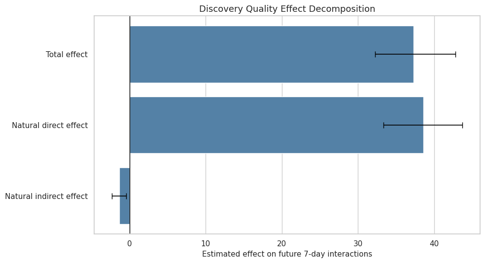

This plot answers the headline mediation question visually: how much of the future-interaction effect appears direct versus routed through same-day satisfaction depth.

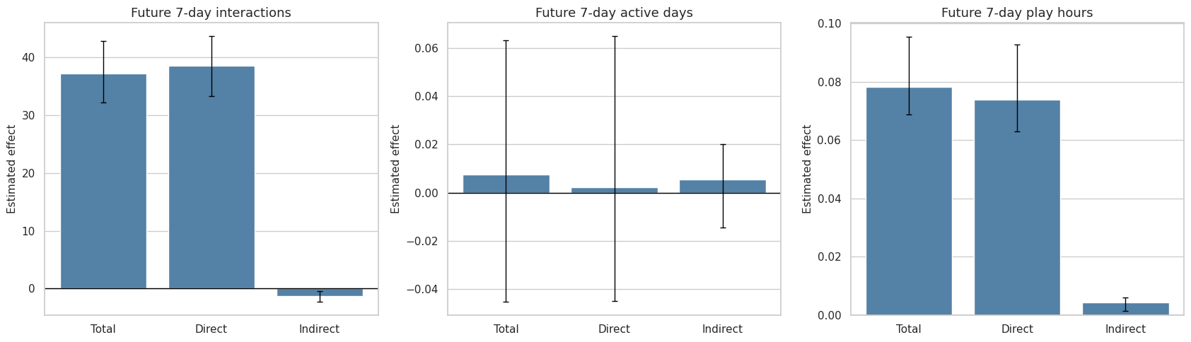
12. Compare Effects Across Outcomes

This cell compares the same decomposition across all three future outcomes. The alternate outcomes help check whether the result is specific to interaction count or whether it also appears for active days and play hours.

outcome_plot = effect_summary.query(
    "estimand in ['gcomp_total_effect', 'natural_direct_effect', 'natural_indirect_effect']"
).copy()
outcome_plot["estimand_label"] = outcome_plot["estimand"].map(
    {
        "gcomp_total_effect": "Total",
        "natural_direct_effect": "Direct",
        "natural_indirect_effect": "Indirect",
    }
)

fig, axes = plt.subplots(1, 3, figsize=(17, 5), sharey=False)
for ax, outcome in zip(axes, OUTCOME_COLUMNS):
    current = outcome_plot.query("outcome == @outcome").copy()
    sns.barplot(data=current, x="estimand_label", y="estimate", color="steelblue", ax=ax)
    for row_index, row in current.reset_index(drop=True).iterrows():
        lower = row["estimate"] - row["ci_95_lower"]
        upper = row["ci_95_upper"] - row["estimate"]
        ax.errorbar(
            x=row_index,
            y=row["estimate"],
            yerr=[[lower], [upper]],
            fmt="none",
            color="black",
            capsize=3,
            linewidth=1,
        )
    ax.axhline(0, color="black", linewidth=1)
    ax.set_title(OUTCOME_LABELS[outcome])
    ax.set_xlabel("")
    ax.set_ylabel("Estimated effect")

plt.tight_layout()
fig.savefig(FIGURE_DIR / "14_effect_decomposition_by_outcome.png", dpi=160, bbox_inches="tight")
plt.show()

display(
    outcome_plot[
        ["outcome_label", "estimand_label", "estimate", "ci_95_lower", "ci_95_upper", "relative_effect"]
    ].round(4)
)

	outcome_label	estimand_label	estimate	ci_95_lower	ci_95_upper	relative_effect
2	Future 7-day interactions	Total	37.2781	32.2444	42.8135	0.1152
3	Future 7-day interactions	Direct	38.5858	33.3634	43.7154	0.1192
4	Future 7-day interactions	Indirect	-1.3077	-2.3047	-0.4290	-0.0036
9	Future 7-day active days	Total	0.0074	-0.0452	0.0631	0.0011
10	Future 7-day active days	Direct	0.0021	-0.0449	0.0648	0.0003
11	Future 7-day active days	Indirect	0.0053	-0.0145	0.0201	0.0008
16	Future 7-day play hours	Total	0.0784	0.0689	0.0954	0.1000
17	Future 7-day play hours	Direct	0.0739	0.0630	0.0927	0.0943
18	Future 7-day play hours	Indirect	0.0044	0.0014	0.0060	0.0051

The outcome comparison is a robustness check on the practical story. Interaction-count effects can be large while active-day effects are small if most users are already active almost every day.

13. Estimate Controlled Direct Effects

This cell summarizes controlled direct effects at low, median, and high satisfaction-depth levels. Unlike the natural direct effect, a controlled direct effect fixes the mediator to a chosen value for everyone. That makes it useful for asking whether discovery exposure has a different direct effect under weak versus strong satisfaction.

controlled_ci = (
    bootstrap_effects.query("estimand == 'gcomp_total_effect'")
    .head(0)
    .copy()
)

# Controlled direct effects are lighter-weight sensitivity summaries, so the notebook reports point estimates.
controlled_direct_effects = weighted_cde.copy()
controlled_direct_effects["mediator_level_label"] = controlled_direct_effects["mediator_level"].map(
    {
        "low_satisfaction_q25": "Low satisfaction (q25)",
        "median_satisfaction_q50": "Median satisfaction (q50)",
        "high_satisfaction_q75": "High satisfaction (q75)",
    }
)

display(controlled_direct_effects.round(4))

	outcome	outcome_label	mediator_level	mediator_value	controlled_direct_effect	uses_weights	mediator_level_label
0	Y_future_interactions	Future 7-day interactions	low_satisfaction_q25	0.5475	39.4525	True	Low satisfaction (q25)
1	Y_future_interactions	Future 7-day interactions	median_satisfaction_q50	0.6174	38.4273	True	Median satisfaction (q50)
2	Y_future_interactions	Future 7-day interactions	high_satisfaction_q75	0.6856	37.4271	True	High satisfaction (q75)
3	Y_future_active_days	Future 7-day active days	low_satisfaction_q25	0.5475	0.0206	True	Low satisfaction (q25)
4	Y_future_active_days	Future 7-day active days	median_satisfaction_q50	0.6174	-0.0013	True	Median satisfaction (q50)
5	Y_future_active_days	Future 7-day active days	high_satisfaction_q75	0.6856	-0.0227	True	High satisfaction (q75)
6	Y_future_play_hours	Future 7-day play hours	low_satisfaction_q25	0.5475	0.0690	True	Low satisfaction (q25)
7	Y_future_play_hours	Future 7-day play hours	median_satisfaction_q50	0.6174	0.0748	True	Median satisfaction (q50)
8	Y_future_play_hours	Future 7-day play hours	high_satisfaction_q75	0.6856	0.0805	True	High satisfaction (q75)

The controlled direct effects show whether the direct discovery effect changes as the satisfaction level is fixed higher or lower. If the direct effect is similar across levels, the treatment-mediator interaction is not driving the main result.

14. Plot Controlled Direct Effects

This cell visualizes the controlled direct effects. The primary outcome is shown as a line across satisfaction levels, which makes it easier to see whether the direct exposure effect depends strongly on mediator level.

primary_cde = controlled_direct_effects.query("outcome == @PRIMARY_OUTCOME").copy()
mediator_level_order = ["Low satisfaction (q25)", "Median satisfaction (q50)", "High satisfaction (q75)"]
primary_cde["mediator_level_label"] = pd.Categorical(
    primary_cde["mediator_level_label"], categories=mediator_level_order, ordered=True
)
primary_cde = primary_cde.sort_values("mediator_level_label")

fig, ax = plt.subplots(figsize=(10, 5))
sns.lineplot(
    data=primary_cde,
    x="mediator_level_label",
    y="controlled_direct_effect",
    marker="o",
    linewidth=2,
    color="steelblue",
    ax=ax,
)
ax.axhline(0, color="black", linewidth=1)
ax.set_title("Controlled Direct Effects at Fixed Satisfaction Levels")
ax.set_xlabel("")
ax.set_ylabel("Effect on future 7-day interactions")
plt.tight_layout()
fig.savefig(FIGURE_DIR / "15_controlled_direct_effects.png", dpi=160, bbox_inches="tight")
plt.show()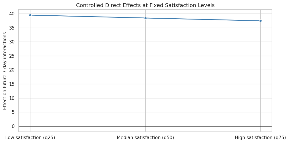

This plot complements the natural direct effect. Natural effects use predicted mediator distributions under treatment states; controlled effects use fixed mediator values that are easier to explain to a broad audience.

15. Inspect Bootstrap Distributions

This cell plots bootstrap distributions for the primary total, direct, and indirect effects. A distribution centered far from zero supports a more stable result; a distribution that crosses zero heavily signals uncertainty.

bootstrap_primary = bootstrap_effects.query(
    "outcome == @PRIMARY_OUTCOME and estimand in ['gcomp_total_effect', 'natural_direct_effect', 'natural_indirect_effect']"
).copy()
bootstrap_primary["estimand_label"] = bootstrap_primary["estimand"].map(
    {
        "gcomp_total_effect": "Total effect",
        "natural_direct_effect": "Natural direct effect",
        "natural_indirect_effect": "Natural indirect effect",
    }
)

fig, axes = plt.subplots(1, 3, figsize=(16, 4.8), sharey=False)
for ax, label in zip(axes, ["Total effect", "Natural direct effect", "Natural indirect effect"]):
    current = bootstrap_primary.query("estimand_label == @label")
    sns.histplot(data=current, x="estimate", bins=35, color="steelblue", edgecolor="white", ax=ax)
    ax.axvline(current["estimate"].mean(), color="black", linestyle="--", linewidth=1)
    ax.axvline(0, color="gray", linewidth=1)
    ax.set_title(label)
    ax.set_xlabel("Bootstrap estimate")
    ax.set_ylabel("Iterations")

plt.tight_layout()
fig.savefig(FIGURE_DIR / "16_bootstrap_effect_distributions.png", dpi=160, bbox_inches="tight")
plt.show()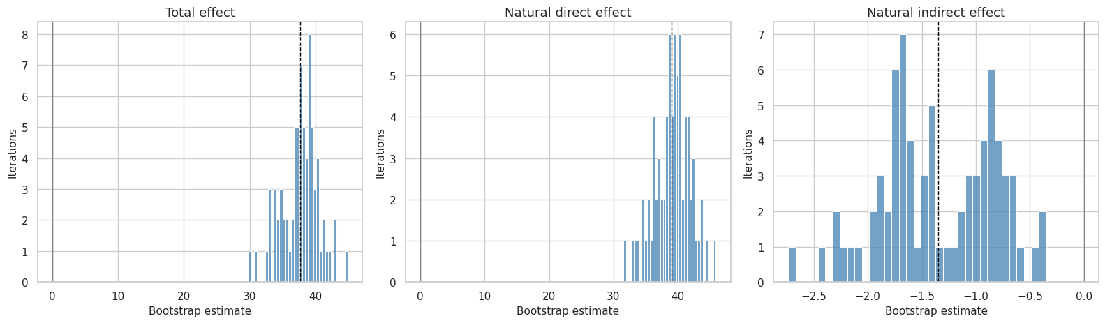

The bootstrap distributions are useful for diagnosing whether the intervals are driven by a few unusual resamples or by broad uncertainty across user clusters.

16. Create a Plain-Language Results Table

This cell creates a compact results table for the writeup. It keeps only the most important primary-outcome rows and gives them readable labels.

plain_language_rows = effect_summary.query(
    "outcome == @PRIMARY_OUTCOME and estimand in ['gcomp_total_effect', 'natural_direct_effect', 'natural_indirect_effect', 'mediator_shift_M1_minus_M0']"
).copy()
plain_language_rows["result_label"] = plain_language_rows["estimand"].map(
    {
        "gcomp_total_effect": "Total effect of high discovery exposure",
        "natural_direct_effect": "Direct effect not routed through satisfaction depth",
        "natural_indirect_effect": "Indirect effect routed through satisfaction depth",
        "mediator_shift_M1_minus_M0": "Estimated shift in satisfaction depth",
    }
)
plain_language_results = plain_language_rows[
    [
        "result_label",
        "estimate",
        "ci_95_lower",
        "ci_95_upper",
        "relative_effect",
        "proportion_mediated",
    ]
].copy()

# The mediator shift is on the mediator scale, so its relative effect and proportion mediated are not directly comparable.
plain_language_results.loc[
    plain_language_results["result_label"].eq("Estimated shift in satisfaction depth"),
    ["relative_effect", "proportion_mediated"],
] = np.nan

display(plain_language_results.round(4))

	result_label	estimate	ci_95_lower	ci_95_upper	relative_effect	proportion_mediated
2	Total effect of high discovery exposure	37.2781	32.2444	42.8135	0.1152	-0.0351
3	Direct effect not routed through satisfaction depth	38.5858	33.3634	43.7154	0.1192	-0.0351
4	Indirect effect routed through satisfaction depth	-1.3077	-2.3047	-0.4290	-0.0036	-0.0351
6	Estimated shift in satisfaction depth	0.0231	0.0185	0.0279	NaN	NaN

This table is the one to use when explaining the result to a non-technical reader. The full tables remain saved for reproducibility, but this version keeps the core story visible.

17. Save Effect Tables and Figures

This cell saves the point estimates, bootstrap draws, confidence-interval summary, controlled direct effects, and model diagnostics. It also mirrors the main tables into the notebook writeup folder.

all_effect_estimates = pd.concat(
    [
        weighted_effects.assign(estimator_variant="weighted_regression"),
        unweighted_effects.assign(estimator_variant="unweighted_regression"),
    ],
    ignore_index=True,
)
all_model_diagnostics = pd.concat(
    [
        weighted_model_diagnostics.assign(estimator_variant="weighted_regression"),
        unweighted_model_diagnostics.assign(estimator_variant="unweighted_regression"),
    ],
    ignore_index=True,
)

all_effect_estimates.to_csv(EFFECT_ESTIMATES_OUTPUT, index=False)
bootstrap_effects.to_csv(BOOTSTRAP_EFFECTS_OUTPUT, index=False)
effect_summary.to_csv(EFFECT_SUMMARY_OUTPUT, index=False)
controlled_direct_effects.to_csv(CONTROLLED_DIRECT_OUTPUT, index=False)
all_model_diagnostics.to_csv(MODEL_DIAGNOSTICS_OUTPUT, index=False)

plain_language_results.to_csv(TABLE_DIR / "direct_indirect_total_primary_results.csv", index=False)
effect_summary.to_csv(TABLE_DIR / "direct_indirect_total_effect_summary.csv", index=False)
controlled_direct_effects.to_csv(TABLE_DIR / "controlled_direct_effects.csv", index=False)
all_model_diagnostics.to_csv(TABLE_DIR / "effect_model_diagnostics.csv", index=False)

saved_outputs = pd.DataFrame(
    {
        "artifact": [
            "effect_estimates",
            "bootstrap_effects",
            "effect_summary",
            "controlled_direct_effects",
            "model_diagnostics",
            "primary_plain_language_results",
        ],
        "path": [
            str(EFFECT_ESTIMATES_OUTPUT),
            str(BOOTSTRAP_EFFECTS_OUTPUT),
            str(EFFECT_SUMMARY_OUTPUT),
            str(CONTROLLED_DIRECT_OUTPUT),
            str(MODEL_DIAGNOSTICS_OUTPUT),
            str(TABLE_DIR / "direct_indirect_total_primary_results.csv"),
        ],
    }
)

display(saved_outputs)

	artifact	path
0	effect_estimates	/home/apex/Documents/ranking_sys/data/processed/kuairec_discovery_quality_effect_estimates.csv
1	bootstrap_effects	/home/apex/Documents/ranking_sys/data/processed/kuairec_discovery_quality_bootstrap_effects.csv
2	effect_summary	/home/apex/Documents/ranking_sys/data/processed/kuairec_discovery_quality_effect_summary.csv
3	controlled_direct_effects	/home/apex/Documents/ranking_sys/data/processed/kuairec_discovery_quality_controlled_direct_effects.csv
4	model_diagnostics	/home/apex/Documents/ranking_sys/data/processed/kuairec_discovery_quality_effect_model_diagnostics.csv
5	primary_plain_language_results	/home/apex/Documents/ranking_sys/notebooks/projects/project_5_discovery_quality_mediation/writeup/tables/direct_indirect_total_primary_results.csv

The saved outputs are the handoff to the next notebook. They contain both the full reproducible estimates and the compact results table that can later feed a final report.

18. Notebook Takeaways

This notebook estimated the discovery-quality mediation effects using transparent g-computation:

• The total effect compares high-discovery and lower-discovery user-days after observed adjustment.
• The natural direct effect captures the pathway not routed through same-day satisfaction depth.
• The natural indirect effect captures the pathway through predicted satisfaction-depth changes.
• User-level bootstrap intervals quantify uncertainty while respecting repeated days per user.
• Alternate outcomes check whether the story is specific to interaction volume or also appears in active days and play time.

The next notebook should focus on robustness and sensitivity: alternative mediator definitions, alternative treatment thresholds, and sensitivity to unobserved mediator-outcome confounding.