Metric Construction and Validation for Discovery Quality

The previous notebook created a user-day panel from KuaiRec and established a causal question: recommendation exposure can drive immediate activity, but product teams usually care about whether that exposure creates meaningful discovery, satisfaction, and durable return behavior. This notebook turns that setup into explicit measurement objects.

The measurement problem is subtle. A click-like metric is easy to increase, but it can reward low-value behavior: curiosity clicks, accidental plays, or short sessions that do not create satisfaction. A discovery-quality metric should do more than count immediate response. It should combine three ideas:

• Discovery exposure: did the user receive less-obvious or broader content, such as long-tail videos or categories they had not recently consumed?
• Satisfaction depth: did the interaction look meaningful, using watch ratio, valid play, completion, and abandonment proxies?
• Future value validation: do higher metric values line up with future activity, while not merely duplicating past activity volume?

A key causal discipline in this notebook is separation of roles. Exposure-like variables are candidates for treatments or policy levers. Satisfaction-like variables are plausible mediators. Future outcomes are used only for validation; they are never used to build the metric itself. That separation keeps later mediation analysis understandable.

1. Load Libraries and Paths

This cell imports the data, plotting, and utility libraries used throughout the notebook. It also defines the raw input paths from the setup notebook and the output paths for the metric panel, validation tables, and figures created here.

from pathlib import Path
import warnings

import numpy as np
import pandas as pd
import seaborn as sns
import matplotlib.pyplot as plt
from IPython.display import display

warnings.filterwarnings("ignore", category=FutureWarning)

# Keep the visual style consistent with the earlier notebooks while staying readable in VS Code/Jupyter.
sns.set_theme(style="whitegrid", context="notebook")
plt.rcParams["figure.figsize"] = (11, 6)
plt.rcParams["axes.titlesize"] = 13
plt.rcParams["axes.labelsize"] = 11
pd.set_option("display.max_columns", 120)
pd.set_option("display.max_colwidth", 120)

# Detect the repository root whether the notebook is run from the repo root or from this notebook folder.
PROJECT_ROOT = Path.cwd().resolve()
while not (PROJECT_ROOT / "data").exists() and PROJECT_ROOT.parent != PROJECT_ROOT:
    PROJECT_ROOT = PROJECT_ROOT.parent

PROCESSED_DIR = PROJECT_ROOT / "data" / "processed"
NOTEBOOK_DIR = PROJECT_ROOT / "notebooks" / "discovery_quality_mediation"
WRITEUP_DIR = NOTEBOOK_DIR / "writeup"
FIGURE_DIR = WRITEUP_DIR / "figures"
TABLE_DIR = WRITEUP_DIR / "tables"

FIGURE_DIR.mkdir(parents=True, exist_ok=True)
TABLE_DIR.mkdir(parents=True, exist_ok=True)

PANEL_INPUT = PROCESSED_DIR / "kuairec_discovery_quality_mediation_panel.parquet"
INTERACTIONS_INPUT = PROCESSED_DIR / "kuairec_discovery_quality_interactions_sample.parquet"
ITEM_FEATURES_INPUT = PROCESSED_DIR / "kuairec_discovery_quality_item_features.parquet"
READINESS_INPUT = PROCESSED_DIR / "kuairec_discovery_quality_readiness.csv"

METRIC_PANEL_OUTPUT = PROCESSED_DIR / "kuairec_discovery_quality_metric_panel.parquet"
METRIC_REGISTRY_OUTPUT = PROCESSED_DIR / "kuairec_discovery_quality_metric_registry.csv"
METRIC_VALIDATION_OUTPUT = PROCESSED_DIR / "kuairec_discovery_quality_metric_validation.csv"
METRIC_CORRELATION_OUTPUT = PROCESSED_DIR / "kuairec_discovery_quality_metric_correlations.csv"
METRIC_DECILE_OUTPUT = PROCESSED_DIR / "kuairec_discovery_quality_metric_deciles.csv"
METRIC_SELECTION_OUTPUT = PROCESSED_DIR / "kuairec_discovery_quality_selected_metrics.csv"

The directories are intentionally the same pattern used by the rest of the repository: durable data artifacts go to data/processed, while notebook-specific tables and figures go to the local writeup folder. That keeps the notebook readable and makes downstream notebooks load a stable artifact instead of recreating everything.

2. Load the Setup Artifacts

This cell loads the active user-day mediation panel and the supporting interaction/item artifacts from the setup notebook. The panel is the main unit of analysis: one row is one active user on one calendar day, with same-day exposure and satisfaction signals plus future engagement outcomes.

metric_base = pd.read_parquet(PANEL_INPUT)
interactions = pd.read_parquet(INTERACTIONS_INPUT)
item_features = pd.read_parquet(ITEM_FEATURES_INPUT)
readiness = pd.read_csv(READINESS_INPUT)

load_summary = pd.DataFrame(
    {
        "artifact": ["mediation_panel", "interaction_sample", "item_features", "readiness_checks"],
        "rows": [len(metric_base), len(interactions), len(item_features), len(readiness)],
        "columns": [metric_base.shape[1], interactions.shape[1], item_features.shape[1], readiness.shape[1]],
    }
)

display(load_summary)
display(readiness)

	artifact	rows	columns
0	mediation_panel	8199	81
1	interaction_sample	440788	37
2	item_features	3327	27
3	readiness_checks	6	3

	check	value	notes
0	active_user_days	8199.000000	Rows available for active-day mediation setup.
1	sampled_users	133.000000	Users represented in the mediation panel.
2	treatment_rate	0.501525	Should be neither near 0 nor near 1.
3	mediator_satisfaction_std	0.176618	Mediator must vary across user-days.
4	future_7day_interactions_std	180.363332	Outcome must vary across user-days.
5	max_key_variable_missing_rate	0.000000	Key variables should be complete or nearly complete.

The readiness table is the first sanity check for this notebook. The treatment rate is close to balanced, the mediator and future outcomes vary, and key missingness is zero. That means metric validation can focus on substantive behavior rather than basic data repair.

3. State the Measurement Contract

Before building formulas, this cell creates a small data dictionary for the key columns used here. This prevents the notebook from becoming a bag of engineered features. Each metric has to map back to a causal role: exposure, mediator, outcome, or history control.

measurement_contract = pd.DataFrame(
    [
        {
            "role": "exposure",
            "column": "discovery_candidate_share",
            "meaning": "Share of same-day interactions that are platform long-tail or first category exposures for the user.",
            "used_for_metric_building": True,
            "uses_future_information": False,
        },
        {
            "role": "exposure",
            "column": "long_tail_share",
            "meaning": "Share of same-day interactions with lower platform-level exposure items.",
            "used_for_metric_building": True,
            "uses_future_information": False,
        },
        {
            "role": "exposure",
            "column": "new_category_share",
            "meaning": "Share of same-day interactions from categories not previously seen for that user in the sampled history.",
            "used_for_metric_building": True,
            "uses_future_information": False,
        },
        {
            "role": "mediator",
            "column": "high_satisfaction_share",
            "meaning": "Share of interactions with watch ratio at least 0.8.",
            "used_for_metric_building": True,
            "uses_future_information": False,
        },
        {
            "role": "mediator",
            "column": "valid_play_share",
            "meaning": "Share of interactions with enough watch time to look like a real play.",
            "used_for_metric_building": True,
            "uses_future_information": False,
        },
        {
            "role": "mediator",
            "column": "short_abandon_share",
            "meaning": "Share of interactions with very low watch ratio, used as a quality guardrail.",
            "used_for_metric_building": True,
            "uses_future_information": False,
        },
        {
            "role": "outcome",
            "column": "outcome_future_7day_interactions",
            "meaning": "Seven-day future interaction count after the current day.",
            "used_for_metric_building": False,
            "uses_future_information": True,
        },
        {
            "role": "outcome",
            "column": "outcome_future_7day_active_days",
            "meaning": "Seven-day future active-day count after the current day.",
            "used_for_metric_building": False,
            "uses_future_information": True,
        },
        {
            "role": "history_control",
            "column": "prior_3day_interactions",
            "meaning": "Recent activity before the current day, used to detect whether a metric merely tracks user activity level.",
            "used_for_metric_building": False,
            "uses_future_information": False,
        },
    ]
)

display(measurement_contract)

	role	column	meaning	used_for_metric_building	uses_future_information
0	exposure	discovery_candidate_share	Share of same-day interactions that are platform long-tail or first category exposures for the user.	True	False
1	exposure	long_tail_share	Share of same-day interactions with lower platform-level exposure items.	True	False
2	exposure	new_category_share	Share of same-day interactions from categories not previously seen for that user in the sampled history.	True	False
3	mediator	high_satisfaction_share	Share of interactions with watch ratio at least 0.8.	True	False
4	mediator	valid_play_share	Share of interactions with enough watch time to look like a real play.	True	False
5	mediator	short_abandon_share	Share of interactions with very low watch ratio, used as a quality guardrail.	True	False
6	outcome	outcome_future_7day_interactions	Seven-day future interaction count after the current day.	False	True
7	outcome	outcome_future_7day_active_days	Seven-day future active-day count after the current day.	False	True
8	history_control	prior_3day_interactions	Recent activity before the current day, used to detect whether a metric merely tracks user activity level.	False	False

The contract makes one important rule explicit: future outcomes validate metrics but do not define them. That is what makes the later evidence more credible. If a metric were built from future behavior, its validation would be circular.

4. Create Normalization Helpers

Metrics are easier to compare when they live on similar scales. This cell defines small helpers for clipping rates, min-max scaling, Spearman correlation, and decile assignment. The helpers also handle constant columns gracefully so the notebook fails less often when the sample changes.

def clip_rate(series):
    """Keep a rate-style series within [0, 1] while preserving missing values."""
    return series.astype(float).clip(lower=0, upper=1)


def minmax_score(series):
    """Scale a numeric series to [0, 1]; return 0.5 if the column has no variation."""
    values = series.astype(float)
    min_value = values.min(skipna=True)
    max_value = values.max(skipna=True)
    if pd.isna(min_value) or pd.isna(max_value) or np.isclose(max_value, min_value):
        return pd.Series(0.5, index=series.index)
    return (values - min_value) / (max_value - min_value)


def safe_spearman(frame, left, right):
    """Spearman correlation with guardrails for constant or missing columns."""
    pair = frame[[left, right]].dropna()
    if len(pair) < 3 or pair[left].nunique() < 2 or pair[right].nunique() < 2:
        return np.nan
    return pair[left].corr(pair[right], method="spearman")


def add_decile(frame, metric):
    """Assign stable deciles even when many rows share the same metric value."""
    ranked = frame[metric].rank(method="first")
    return pd.qcut(ranked, q=10, labels=False, duplicates="drop") + 1

helper_summary = pd.DataFrame(
    {
        "helper": ["clip_rate", "minmax_score", "safe_spearman", "add_decile"],
        "purpose": [
            "Protect rate-like inputs from drifting outside [0, 1].",
            "Place count or score variables on a comparable [0, 1] scale.",
            "Compute rank correlation without breaking on degenerate columns.",
            "Create ordered metric groups for top-versus-bottom validation.",
        ],
    }
)

display(helper_summary)

	helper	purpose
0	clip_rate	Protect rate-like inputs from drifting outside [0, 1].
1	minmax_score	Place count or score variables on a comparable [0, 1] scale.
2	safe_spearman	Compute rank correlation without breaking on degenerate columns.
3	add_decile	Create ordered metric groups for top-versus-bottom validation.

These helpers are deliberately simple. The goal is not to hide modeling complexity; it is to make each metric definition readable and reproducible. Later notebooks can replace a hand-built score with learned weights, but this notebook starts with transparent measurement.

5. Build Metric Components

This cell prepares reusable components from the user-day panel. Some columns are already rates; others need transformation. For example, raw interaction counts are converted to a scaled log-volume score so high-volume days matter without letting extreme activity dominate every metric.

metric_panel = metric_base.copy()
metric_panel = metric_panel.sort_values(["user_id", "event_date"]).reset_index(drop=True)

# Category breadth is another discovery signal: a day with many categories per interaction is broader.
metric_panel["category_breadth_rate"] = (
    metric_panel["unique_categories"] / metric_panel["interactions"].replace(0, np.nan)
).fillna(0)
metric_panel["category_breadth_rate"] = clip_rate(metric_panel["category_breadth_rate"])

# Scaled volume keeps activity information available without treating raw clicks as the target metric.
metric_panel["engagement_volume_score"] = minmax_score(np.log1p(metric_panel["interactions"]))
metric_panel["recent_activity_score"] = minmax_score(np.log1p(metric_panel["prior_3day_interactions"]))

rate_inputs = [
    "discovery_candidate_share",
    "long_tail_share",
    "new_category_share",
    "valid_play_share",
    "high_satisfaction_share",
    "complete_or_rewatch_share",
    "short_abandon_share",
    "avg_satisfaction_score",
]
for col in rate_inputs:
    metric_panel[col] = clip_rate(metric_panel[col])

component_summary = metric_panel[
    [
        "category_breadth_rate",
        "engagement_volume_score",
        "recent_activity_score",
        "discovery_candidate_share",
        "long_tail_share",
        "new_category_share",
        "valid_play_share",
        "high_satisfaction_share",
        "complete_or_rewatch_share",
        "short_abandon_share",
        "avg_satisfaction_score",
    ]
].describe(percentiles=[0.1, 0.25, 0.5, 0.75, 0.9]).T

display(component_summary)

	count	mean	std	min	10%	25%	50%	75%	90%	max
category_breadth_rate	8199.0	0.426961	0.163345	0.105802	0.257732	0.313433	0.396226	0.500000	0.625000	1.0
engagement_volume_score	8199.0	0.608386	0.157664	0.000000	0.416686	0.535855	0.640961	0.715275	0.771506	1.0
recent_activity_score	8199.0	0.774028	0.143744	0.000000	0.629895	0.733243	0.808920	0.857085	0.892857	1.0
discovery_candidate_share	8199.0	0.364368	0.172628	0.000000	0.090909	0.271010	0.390244	0.480570	0.555556	1.0
long_tail_share	8199.0	0.351875	0.164697	0.000000	0.090909	0.260572	0.377551	0.466667	0.539474	1.0
new_category_share	8199.0	0.020453	0.085513	0.000000	0.000000	0.000000	0.000000	0.000000	0.029733	1.0
valid_play_share	8199.0	0.939417	0.095783	0.000000	0.830717	0.920000	0.975610	1.000000	1.000000	1.0
high_satisfaction_share	8199.0	0.468649	0.176618	0.000000	0.257489	0.349699	0.461538	0.575758	0.692308	1.0
complete_or_rewatch_share	8199.0	0.323119	0.171901	0.000000	0.128968	0.208333	0.302326	0.412944	0.533537	1.0
short_abandon_share	8199.0	0.101160	0.100637	0.000000	0.000000	0.037736	0.076923	0.133333	0.214286	1.0
avg_satisfaction_score	8199.0	0.524125	0.101305	0.000000	0.409583	0.460297	0.516842	0.578268	0.647112	1.0

The components cover three different measurement families: breadth of discovery, depth of satisfaction, and volume of immediate activity. Keeping these separate lets us later ask whether a composite metric is truly adding information or just renaming clicks.

6. Construct Candidate Discovery-Quality Metrics

This cell creates the candidate metrics. The formulas are transparent on purpose:

• discovery_breadth_score is exposure-like and can support treatment definitions.
• satisfaction_depth_score is mediator-like and should not be treated as pre-exposure.
• quality_adjusted_discovery_score combines discovery and satisfaction, making it useful as a product metric but not as a clean treatment in mediation.
• shallow_click_pressure_score is a guardrail: high immediate volume paired with weak satisfaction.

metric_panel["discovery_breadth_score"] = clip_rate(
    0.45 * metric_panel["discovery_candidate_share"]
    + 0.30 * metric_panel["long_tail_share"]
    + 0.15 * metric_panel["new_category_share"]
    + 0.10 * metric_panel["category_breadth_rate"]
)

metric_panel["satisfaction_depth_score"] = clip_rate(
    0.30 * metric_panel["high_satisfaction_share"]
    + 0.25 * metric_panel["valid_play_share"]
    + 0.20 * metric_panel["avg_satisfaction_score"]
    + 0.15 * metric_panel["complete_or_rewatch_share"]
    + 0.10 * (1 - metric_panel["short_abandon_share"])
)

metric_panel["quality_adjusted_discovery_score"] = np.sqrt(
    metric_panel["discovery_breadth_score"] * metric_panel["satisfaction_depth_score"]
)

metric_panel["balanced_discovery_quality_score"] = clip_rate(
    0.50 * metric_panel["discovery_breadth_score"]
    + 0.50 * metric_panel["satisfaction_depth_score"]
)

metric_panel["volume_weighted_quality_score"] = minmax_score(
    np.log1p(metric_panel["interactions"]) * metric_panel["quality_adjusted_discovery_score"]
)

metric_panel["shallow_click_pressure_score"] = clip_rate(
    metric_panel["engagement_volume_score"] * (1 - metric_panel["satisfaction_depth_score"])
)

# These binary flags are convenient for summaries. Only the discovery-breadth flag is exposure-like.
metric_panel["high_discovery_breadth_day"] = (
    metric_panel["discovery_breadth_score"] >= metric_panel["discovery_breadth_score"].median()
).astype("int8")
metric_panel["high_quality_adjusted_discovery_day"] = (
    metric_panel["quality_adjusted_discovery_score"] >= metric_panel["quality_adjusted_discovery_score"].median()
).astype("int8")

candidate_metrics = [
    "discovery_breadth_score",
    "satisfaction_depth_score",
    "quality_adjusted_discovery_score",
    "balanced_discovery_quality_score",
    "volume_weighted_quality_score",
    "shallow_click_pressure_score",
]

metric_registry = pd.DataFrame(
    [
        {
            "metric": "discovery_breadth_score",
            "role": "exposure_like",
            "formula_summary": "Weighted mix of discovery-candidate, long-tail, new-category, and category-breadth rates.",
            "causal_use": "Candidate exposure/treatment measure for later mediation.",
            "caution": "Still observational; high discovery days may reflect user preference and recommender selection.",
        },
        {
            "metric": "satisfaction_depth_score",
            "role": "mediator_like",
            "formula_summary": "Weighted mix of high watch ratio, valid plays, satisfaction score, completion, and low abandonment.",
            "causal_use": "Candidate mediator between discovery exposure and future value.",
            "caution": "Post-exposure signal; do not use as a pre-treatment control.",
        },
        {
            "metric": "quality_adjusted_discovery_score",
            "role": "composite_product_metric",
            "formula_summary": "Geometric mean of discovery breadth and satisfaction depth.",
            "causal_use": "Useful for monitoring and policy ranking; not a clean treatment in mediation.",
            "caution": "Combines exposure and mediator information.",
        },
        {
            "metric": "balanced_discovery_quality_score",
            "role": "composite_product_metric",
            "formula_summary": "Arithmetic average of discovery breadth and satisfaction depth.",
            "causal_use": "Transparent composite metric for comparison with the geometric version.",
            "caution": "Can look good when only one component is high.",
        },
        {
            "metric": "volume_weighted_quality_score",
            "role": "business_metric",
            "formula_summary": "Quality-adjusted discovery scaled by same-day log interaction volume.",
            "causal_use": "Useful for product prioritization where scale matters.",
            "caution": "More click-sensitive than the pure quality metrics.",
        },
        {
            "metric": "shallow_click_pressure_score",
            "role": "guardrail",
            "formula_summary": "High immediate volume combined with low satisfaction depth.",
            "causal_use": "Negative signal or guardrail for click-heavy recommendation behavior.",
            "caution": "A high value is bad; correlations should be read with the sign reversed.",
        },
    ]
)

metric_distribution = metric_panel[candidate_metrics].describe(percentiles=[0.1, 0.25, 0.5, 0.75, 0.9]).T

display(metric_registry)
display(metric_distribution)

	metric	role	formula_summary	causal_use	caution
0	discovery_breadth_score	exposure_like	Weighted mix of discovery-candidate, long-tail, new-category, and category-breadth rates.	Candidate exposure/treatment measure for later mediation.	Still observational; high discovery days may reflect user preference and recommender selection.
1	satisfaction_depth_score	mediator_like	Weighted mix of high watch ratio, valid plays, satisfaction score, completion, and low abandonment.	Candidate mediator between discovery exposure and future value.	Post-exposure signal; do not use as a pre-treatment control.
2	quality_adjusted_discovery_score	composite_product_metric	Geometric mean of discovery breadth and satisfaction depth.	Useful for monitoring and policy ranking; not a clean treatment in mediation.	Combines exposure and mediator information.
3	balanced_discovery_quality_score	composite_product_metric	Arithmetic average of discovery breadth and satisfaction depth.	Transparent composite metric for comparison with the geometric version.	Can look good when only one component is high.
4	volume_weighted_quality_score	business_metric	Quality-adjusted discovery scaled by same-day log interaction volume.	Useful for product prioritization where scale matters.	More click-sensitive than the pure quality metrics.
5	shallow_click_pressure_score	guardrail	High immediate volume combined with low satisfaction depth.	Negative signal or guardrail for click-heavy recommendation behavior.	A high value is bad; correlations should be read with the sign reversed.

	count	mean	std	min	10%	25%	50%	75%	90%	max
discovery_breadth_score	8199.0	0.315292	0.122804	0.022222	0.122665	0.247618	0.330000	0.395932	0.452737	0.925000
satisfaction_depth_score	8199.0	0.618626	0.112600	0.000000	0.482869	0.547525	0.617436	0.685637	0.753525	1.000000
quality_adjusted_discovery_score	8199.0	0.429600	0.106185	0.000000	0.275625	0.374607	0.443178	0.499683	0.548292	0.921954
balanced_discovery_quality_score	8199.0	0.466959	0.085621	0.050000	0.359290	0.413900	0.470779	0.523202	0.569368	0.925000
volume_weighted_quality_score	8199.0	0.487750	0.167229	0.000000	0.227026	0.400079	0.518041	0.605890	0.674227	1.000000
shallow_click_pressure_score	8199.0	0.233236	0.089682	0.000000	0.116157	0.178974	0.236637	0.291770	0.341866	0.614382

The registry is the most important table in the notebook. It says which metrics are appropriate for causal exposure analysis and which ones are better treated as mediators or monitoring metrics. That distinction prevents post-treatment leakage in later notebooks.

7. Visualize Metric Distributions

A metric that is almost always the same value is not useful for causal analysis or product monitoring. This cell plots each candidate metric distribution so we can see spread, skew, and whether any score collapses to a narrow band.

metric_long = metric_panel[candidate_metrics].melt(var_name="metric", value_name="value")

metric_name_order = [
    "discovery_breadth_score",
    "satisfaction_depth_score",
    "quality_adjusted_discovery_score",
    "balanced_discovery_quality_score",
    "volume_weighted_quality_score",
    "shallow_click_pressure_score",
]

fig, axes = plt.subplots(3, 2, figsize=(14, 11), sharex=False)
axes = axes.flatten()
for ax, metric in zip(axes, metric_name_order):
    sns.histplot(
        data=metric_long.query("metric == @metric"),
        x="value",
        bins=35,
        color="steelblue",
        edgecolor="white",
        ax=ax,
    )
    ax.axvline(metric_panel[metric].median(), color="black", linestyle="--", linewidth=1)
    ax.set_title(metric.replace("_", " ").title())
    ax.set_xlabel("Score")
    ax.set_ylabel("User-days")

plt.tight_layout()
fig.savefig(FIGURE_DIR / "05_metric_distributions.png", dpi=160, bbox_inches="tight")
plt.show()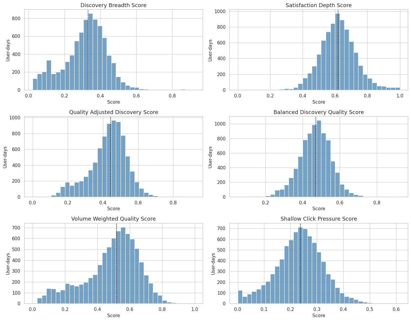

The distributions show whether the metrics provide enough variation for grouping and modeling. The median reference line is also a practical reminder that later binary contrasts should be based on a score with real spread, not on a degenerate indicator.

8. Check Same-Day Metric Relationships

This cell calculates correlations among candidate metrics and the raw same-day components. The purpose is to understand what each metric is mostly measuring. A good composite should relate to discovery and satisfaction, while the guardrail should move in the opposite direction from satisfaction.

same_day_columns = candidate_metrics + [
    "interactions",
    "engagement_volume_score",
    "discovery_candidate_share",
    "long_tail_share",
    "new_category_share",
    "category_breadth_rate",
    "valid_play_share",
    "high_satisfaction_share",
    "complete_or_rewatch_share",
    "short_abandon_share",
]

same_day_correlation = metric_panel[same_day_columns].corr(method="spearman")

fig, ax = plt.subplots(figsize=(13, 10))
sns.heatmap(
    same_day_correlation,
    cmap="coolwarm",
    center=0,
    linewidths=0.4,
    cbar_kws={"label": "Spearman correlation"},
    ax=ax,
)
ax.set_title("Same-Day Metric and Component Relationships")
plt.tight_layout()
fig.savefig(FIGURE_DIR / "06_same_day_metric_correlation_heatmap.png", dpi=160, bbox_inches="tight")
plt.show()

display(same_day_correlation.round(3))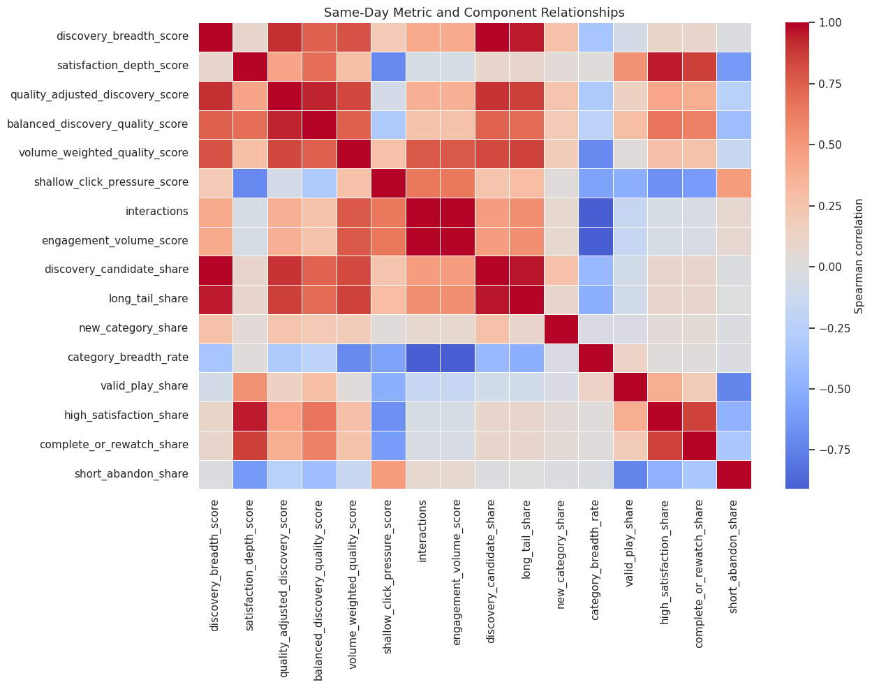

	discovery_breadth_score	satisfaction_depth_score	quality_adjusted_discovery_score	balanced_discovery_quality_score	volume_weighted_quality_score	shallow_click_pressure_score	interactions	engagement_volume_score	discovery_candidate_share	long_tail_share	new_category_share	category_breadth_rate	valid_play_share	high_satisfaction_share	complete_or_rewatch_share	short_abandon_share
discovery_breadth_score	1.000	0.093	0.904	0.745	0.792	0.208	0.410	0.410	0.993	0.949	0.263	-0.344	-0.069	0.108	0.101	-0.013
satisfaction_depth_score	0.093	1.000	0.439	0.688	0.289	-0.713	-0.052	-0.052	0.090	0.083	0.033	0.019	0.535	0.955	0.864	-0.617
quality_adjusted_discovery_score	0.904	0.439	1.000	0.934	0.838	-0.073	0.373	0.373	0.898	0.859	0.251	-0.313	0.142	0.431	0.392	-0.241
balanced_discovery_quality_score	0.745	0.688	0.934	1.000	0.742	-0.310	0.255	0.255	0.737	0.700	0.208	-0.220	0.292	0.669	0.611	-0.405
volume_weighted_quality_score	0.792	0.289	0.838	0.742	1.000	0.268	0.774	0.774	0.833	0.852	0.183	-0.702	0.028	0.282	0.258	-0.152
shallow_click_pressure_score	0.208	-0.713	-0.073	-0.310	0.268	1.000	0.655	0.655	0.254	0.300	0.027	-0.569	-0.498	-0.682	-0.611	0.488
interactions	0.410	-0.052	0.373	0.255	0.774	0.655	1.000	1.000	0.482	0.550	0.063	-0.910	-0.160	-0.049	-0.041	0.060
engagement_volume_score	0.410	-0.052	0.373	0.255	0.774	0.655	1.000	1.000	0.482	0.550	0.063	-0.910	-0.160	-0.049	-0.041	0.060
discovery_candidate_share	0.993	0.090	0.898	0.737	0.833	0.254	0.482	0.482	1.000	0.956	0.269	-0.430	-0.079	0.104	0.098	-0.012
long_tail_share	0.949	0.083	0.859	0.700	0.852	0.300	0.550	0.550	0.956	1.000	0.105	-0.497	-0.085	0.097	0.090	-0.006
new_category_share	0.263	0.033	0.251	0.208	0.183	0.027	0.063	0.063	0.269	0.105	1.000	-0.032	-0.032	0.036	0.040	-0.020
category_breadth_rate	-0.344	0.019	-0.313	-0.220	-0.702	-0.569	-0.910	-0.910	-0.430	-0.497	-0.032	1.000	0.133	0.017	0.010	-0.025
valid_play_share	-0.069	0.535	0.142	0.292	0.028	-0.498	-0.160	-0.160	-0.079	-0.085	-0.032	0.133	1.000	0.391	0.199	-0.726
high_satisfaction_share	0.108	0.955	0.431	0.669	0.282	-0.682	-0.049	-0.049	0.104	0.097	0.036	0.017	0.391	1.000	0.857	-0.479
complete_or_rewatch_share	0.101	0.864	0.392	0.611	0.258	-0.611	-0.041	-0.041	0.098	0.090	0.040	0.010	0.199	0.857	1.000	-0.327
short_abandon_share	-0.013	-0.617	-0.241	-0.405	-0.152	0.488	0.060	0.060	-0.012	-0.006	-0.020	-0.025	-0.726	-0.479	-0.327	1.000

This view is a measurement audit. If two metrics are nearly identical, one may be redundant. If the shallow-click guardrail is strongly related to volume and negatively related to satisfaction, it is behaving as intended.

9. Validate Against Future Outcomes

Future outcomes are not part of the metric formulas, so they can be used as validation targets. This cell measures how each candidate metric relates to future seven-day interactions, future active days, and future play hours using Spearman correlations.

future_outcomes = [
    "outcome_future_7day_interactions",
    "outcome_future_7day_active_days",
    "outcome_future_7day_play_hours",
]

future_validation_rows = []
for metric in candidate_metrics:
    for outcome in future_outcomes:
        future_validation_rows.append(
            {
                "metric": metric,
                "validation_target": outcome,
                "spearman_corr": safe_spearman(metric_panel, metric, outcome),
            }
        )

future_validation = pd.DataFrame(future_validation_rows)
future_validation_wide = future_validation.pivot(
    index="metric", columns="validation_target", values="spearman_corr"
).reset_index()

display(future_validation_wide.round(3))

validation_target	metric	outcome_future_7day_active_days	outcome_future_7day_interactions	outcome_future_7day_play_hours
0	balanced_discovery_quality_score	0.282	0.403	0.479
1	discovery_breadth_score	0.398	0.567	0.539
2	quality_adjusted_discovery_score	0.386	0.527	0.564
3	satisfaction_depth_score	-0.009	0.009	0.152
4	shallow_click_pressure_score	0.341	0.392	0.262
5	volume_weighted_quality_score	0.450	0.665	0.672

These correlations are descriptive, not causal estimates. They answer a narrower question: do the candidate metrics point in the same direction as future value? A metric can pass this validation and still require causal adjustment later.

10. Compare Metric Deciles to Future Behavior

Correlation is useful, but product teams often reason in ranked groups. This cell assigns each user-day to metric deciles and compares future outcomes across the ranked distribution. The top-minus-bottom contrast is an intuitive validation check: higher metric days should generally be followed by better future outcomes, except for the shallow-click guardrail where lower is preferable.

decile_frames = []
metric_panel_with_deciles = metric_panel.copy()

for metric in candidate_metrics:
    decile_col = f"{metric}_decile"
    metric_panel_with_deciles[decile_col] = add_decile(metric_panel_with_deciles, metric)
    decile_summary = (
        metric_panel_with_deciles.groupby(decile_col, observed=True)
        .agg(
            user_days=("user_id", "size"),
            metric_mean=(metric, "mean"),
            future_interactions_mean=("outcome_future_7day_interactions", "mean"),
            future_active_days_mean=("outcome_future_7day_active_days", "mean"),
            future_play_hours_mean=("outcome_future_7day_play_hours", "mean"),
            same_day_satisfaction_mean=("satisfaction_depth_score", "mean"),
            same_day_discovery_mean=("discovery_breadth_score", "mean"),
        )
        .reset_index()
        .rename(columns={decile_col: "decile"})
    )
    decile_summary["metric"] = metric
    decile_frames.append(decile_summary)

metric_deciles = pd.concat(decile_frames, ignore_index=True)

decile_lift_rows = []
for metric in candidate_metrics:
    current = metric_deciles.query("metric == @metric").sort_values("decile")
    bottom = current.iloc[0]
    top = current.iloc[-1]
    decile_lift_rows.append(
        {
            "metric": metric,
            "bottom_decile_future_interactions": bottom["future_interactions_mean"],
            "top_decile_future_interactions": top["future_interactions_mean"],
            "top_minus_bottom_future_interactions": top["future_interactions_mean"] - bottom["future_interactions_mean"],
            "top_minus_bottom_future_active_days": top["future_active_days_mean"] - bottom["future_active_days_mean"],
            "top_minus_bottom_future_play_hours": top["future_play_hours_mean"] - bottom["future_play_hours_mean"],
            "top_minus_bottom_same_day_satisfaction": top["same_day_satisfaction_mean"] - bottom["same_day_satisfaction_mean"],
        }
    )

decile_lift = pd.DataFrame(decile_lift_rows).sort_values(
    "top_minus_bottom_future_interactions", ascending=False
)

display(decile_lift.round(3))
display(metric_deciles.head(12).round(3))

	metric	bottom_decile_future_interactions	top_decile_future_interactions	top_minus_bottom_future_interactions	top_minus_bottom_future_active_days	top_minus_bottom_future_play_hours	top_minus_bottom_same_day_satisfaction
4	volume_weighted_quality_score	52.346	484.152	431.806	3.621	1.082	0.082
0	discovery_breadth_score	58.174	426.412	368.238	2.918	0.860	0.022
2	quality_adjusted_discovery_score	66.829	416.454	349.624	2.648	0.902	0.150
5	shallow_click_pressure_score	137.513	421.743	284.229	2.672	0.504	-0.278
3	balanced_discovery_quality_score	137.749	402.717	264.968	1.763	0.749	0.270
1	satisfaction_depth_score	290.466	267.062	-23.404	-0.051	0.148	0.403

	decile	user_days	metric_mean	future_interactions_mean	future_active_days_mean	future_play_hours_mean	same_day_satisfaction_mean	same_day_discovery_mean	metric
0	1	820	0.080	58.174	3.830	0.146	0.628	0.080	discovery_breadth_score
1	2	820	0.175	175.549	6.187	0.437	0.614	0.175	discovery_breadth_score
2	3	820	0.246	294.405	6.705	0.715	0.599	0.246	discovery_breadth_score
3	4	820	0.286	354.070	6.788	0.852	0.601	0.286	discovery_breadth_score
4	5	820	0.317	380.283	6.870	0.924	0.610	0.317	discovery_breadth_score
5	6	819	0.343	403.112	6.829	0.973	0.614	0.343	discovery_breadth_score
6	7	820	0.368	427.234	6.901	1.028	0.624	0.368	discovery_breadth_score
7	8	820	0.396	442.509	6.904	1.051	0.620	0.396	discovery_breadth_score
8	9	820	0.429	445.273	6.902	1.057	0.627	0.429	discovery_breadth_score
9	10	820	0.514	426.412	6.749	1.006	0.650	0.514	discovery_breadth_score
10	1	820	0.423	290.466	5.955	0.625	0.423	0.279	satisfaction_depth_score
11	2	820	0.509	331.652	6.530	0.720	0.509	0.305	satisfaction_depth_score

The decile table translates metrics into rank-order behavior. This is especially useful for storytelling: it shows what happens when we move from low-score user-days to high-score user-days without requiring the reader to parse model coefficients yet.

11. Plot Future Outcomes by Metric Decile

This cell turns the decile table into a compact visual comparison. A clean upward pattern suggests that the metric ranks user-days in a way that is aligned with future engagement. A flat or reversed pattern suggests the metric may be noisy, redundant, or potentially harmful as an optimization target.

plot_metrics = [
    "discovery_breadth_score",
    "satisfaction_depth_score",
    "quality_adjusted_discovery_score",
    "shallow_click_pressure_score",
]
plot_deciles = metric_deciles.query("metric in @plot_metrics").copy()
plot_deciles["metric_label"] = plot_deciles["metric"].str.replace("_", " ").str.title()

fig, axes = plt.subplots(2, 2, figsize=(15, 10), sharex=True)
axes = axes.flatten()
for ax, metric in zip(axes, plot_metrics):
    current = plot_deciles.query("metric == @metric")
    sns.lineplot(
        data=current,
        x="decile",
        y="future_interactions_mean",
        marker="o",
        color="steelblue",
        ax=ax,
    )
    ax.set_title(metric.replace("_", " ").title())
    ax.set_xlabel("Metric decile")
    ax.set_ylabel("Mean future 7-day interactions")
    ax.set_xticks(range(1, 11))

plt.tight_layout()
fig.savefig(FIGURE_DIR / "07_metric_decile_future_outcomes.png", dpi=160, bbox_inches="tight")
plt.show()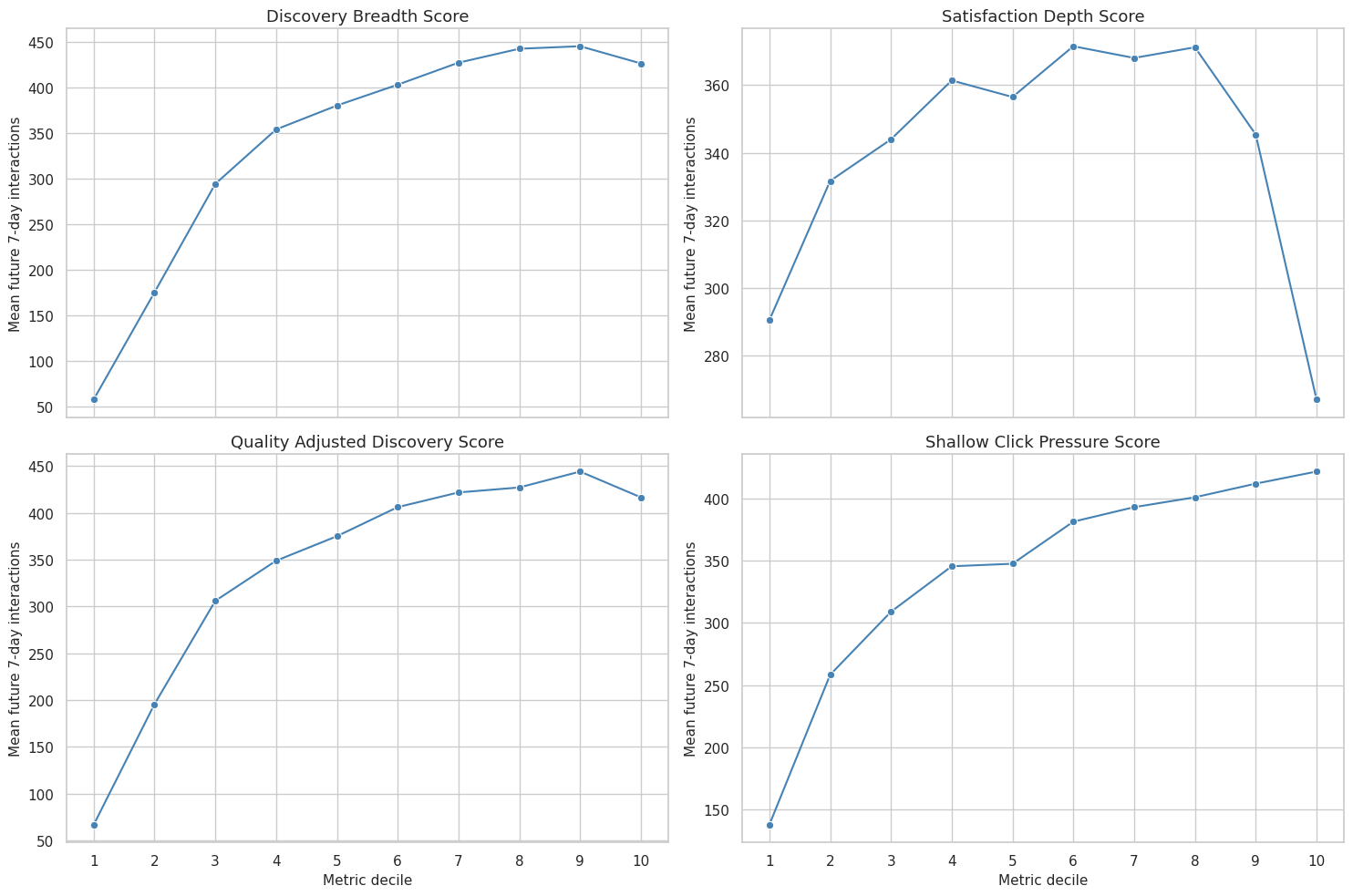

The decile curves make the validation question visible. For the guardrail metric, a high score means shallow click pressure, so a weaker or negative relationship with future outcomes can be a good sign rather than a failure.

12. Measure Stability Across Adjacent User Days

A useful product metric should not be pure noise. This cell computes lag-one stability within each user: how much today’s metric resembles yesterday’s metric. High stability is not automatically better, but a completely unstable metric may be hard to interpret or optimize.

stability_panel = metric_panel.sort_values(["user_id", "event_date"]).copy()
stability_rows = []

for metric in candidate_metrics:
    lag_col = f"lag_1_{metric}"
    stability_panel[lag_col] = stability_panel.groupby("user_id")[metric].shift(1)
    pair = stability_panel[["user_id", metric, lag_col]].dropna()
    lag_corr = np.nan
    if len(pair) >= 3 and pair[metric].nunique() > 1 and pair[lag_col].nunique() > 1:
        lag_corr = pair[metric].corr(pair[lag_col], method="spearman")

    user_means = stability_panel.groupby("user_id")[metric].mean()
    user_stds = stability_panel.groupby("user_id")[metric].std()
    stability_rows.append(
        {
            "metric": metric,
            "lag_1_spearman": lag_corr,
            "mean_within_user_std": user_stds.mean(),
            "between_user_std_of_means": user_means.std(),
            "overall_std": stability_panel[metric].std(),
        }
    )

metric_stability = pd.DataFrame(stability_rows).sort_values("lag_1_spearman", ascending=False)

display(metric_stability.round(3))

	metric	lag_1_spearman	mean_within_user_std	between_user_std_of_means	overall_std
4	volume_weighted_quality_score	0.683	0.165	0.029	0.167
5	shallow_click_pressure_score	0.645	0.078	0.041	0.090
1	satisfaction_depth_score	0.618	0.086	0.068	0.113
2	quality_adjusted_discovery_score	0.589	0.103	0.025	0.106
3	balanced_discovery_quality_score	0.573	0.078	0.035	0.086
0	discovery_breadth_score	0.551	0.123	0.010	0.123

Stability helps separate durable user preference signals from one-off daily noise. In later modeling, highly stable metrics may need stronger user-history adjustment, while very unstable metrics may need smoothing or larger samples.

13. Check Dependence on Past Activity

A metric can look predictive simply because active users stay active. This cell checks how strongly each metric correlates with recent user history. A metric that predicts future outcomes while only moderately tracking past activity is more interesting than one that is just a disguised activity count.

history_columns = [
    "prior_3day_interactions",
    "recent_activity_score",
    "prior_3day_high_satisfaction_share",
    "prior_3day_discovery_candidate_share",
]

history_rows = []
for metric in candidate_metrics:
    for history_col in history_columns:
        history_rows.append(
            {
                "metric": metric,
                "history_variable": history_col,
                "spearman_corr": safe_spearman(metric_panel, metric, history_col),
            }
        )

history_dependence = pd.DataFrame(history_rows)
history_dependence_wide = history_dependence.pivot(
    index="metric", columns="history_variable", values="spearman_corr"
).reset_index()

display(history_dependence_wide.round(3))

history_variable	metric	prior_3day_discovery_candidate_share	prior_3day_high_satisfaction_share	prior_3day_interactions	recent_activity_score
0	balanced_discovery_quality_score	0.348	0.358	0.248	0.248
1	discovery_breadth_score	0.498	-0.027	0.401	0.401
2	quality_adjusted_discovery_score	0.463	0.203	0.357	0.357
3	satisfaction_depth_score	0.005	0.584	-0.046	-0.046
4	shallow_click_pressure_score	0.369	-0.410	0.444	0.444
5	volume_weighted_quality_score	0.598	0.177	0.565	0.565

This table is not trying to remove confounding yet. It is a diagnostic. If a candidate metric is very close to recent activity, future causal notebooks should be especially careful with user fixed effects, lag controls, or doubly robust adjustment.

14. Summarize Metric Validation Evidence

This cell combines distribution quality, future-outcome alignment, decile lift, stability, and history dependence into one validation table. The table is not a final model ranking. It is a structured way to decide which metrics deserve to move forward.

distribution_checks = (
    metric_panel[candidate_metrics]
    .agg(["mean", "std", "min", "max"])
    .T.reset_index()
    .rename(columns={"index": "metric", "std": "metric_std"})
)
distribution_checks["missing_rate"] = metric_panel[candidate_metrics].isna().mean().values

future_score = future_validation_wide.rename(
    columns={
        "outcome_future_7day_interactions": "future_interactions_corr",
        "outcome_future_7day_active_days": "future_active_days_corr",
        "outcome_future_7day_play_hours": "future_play_hours_corr",
    }
)

history_score = history_dependence_wide.rename(
    columns={
        "prior_3day_interactions": "prior_interactions_corr",
        "recent_activity_score": "recent_activity_corr",
        "prior_3day_high_satisfaction_share": "prior_satisfaction_corr",
        "prior_3day_discovery_candidate_share": "prior_discovery_corr",
    }
)

validation_summary = (
    distribution_checks.merge(future_score, on="metric", how="left")
    .merge(history_score, on="metric", how="left")
    .merge(decile_lift, on="metric", how="left")
    .merge(metric_stability, on="metric", how="left")
)

validation_summary["future_alignment_score"] = validation_summary[
    ["future_interactions_corr", "future_active_days_corr", "future_play_hours_corr"]
].mean(axis=1)
validation_summary["history_dependence_score"] = validation_summary[
    ["prior_interactions_corr", "recent_activity_corr"]
].abs().mean(axis=1)
validation_summary["screening_score"] = (
    validation_summary["future_alignment_score"]
    - 0.35 * validation_summary["history_dependence_score"]
)

validation_summary = validation_summary.sort_values("screening_score", ascending=False)

display(
    validation_summary[
        [
            "metric",
            "metric_std",
            "future_alignment_score",
            "history_dependence_score",
            "screening_score",
            "top_minus_bottom_future_interactions",
            "lag_1_spearman",
            "missing_rate",
        ]
    ].round(3)
)

	metric	metric_std	future_alignment_score	history_dependence_score	screening_score	top_minus_bottom_future_interactions	lag_1_spearman	missing_rate
4	volume_weighted_quality_score	0.167	0.596	0.565	0.398	431.806	0.683	0.0
2	quality_adjusted_discovery_score	0.106	0.492	0.357	0.367	349.624	0.589	0.0
0	discovery_breadth_score	0.123	0.502	0.401	0.361	368.238	0.551	0.0
3	balanced_discovery_quality_score	0.086	0.388	0.248	0.301	264.968	0.573	0.0
5	shallow_click_pressure_score	0.090	0.332	0.444	0.176	284.229	0.645	0.0
1	satisfaction_depth_score	0.113	0.051	0.046	0.035	-23.404	0.618	0.0

The screening score is deliberately lightweight. It rewards future alignment and penalizes dependence on recent activity, but it is not a replacement for causal estimation. Its job is to narrow attention to the metrics that are worth modeling next.

15. Visualize the Validation Summary

This cell creates a figure that places future alignment and history dependence side by side. The best candidates are usually those with meaningful future alignment and tolerable dependence on prior activity. The guardrail metric should be read differently because high values represent worse quality pressure.

summary_plot = validation_summary.copy()
summary_plot["metric_label"] = summary_plot["metric"].str.replace("_", " ").str.title()
summary_long = summary_plot.melt(
    id_vars=["metric", "metric_label"],
    value_vars=["future_alignment_score", "history_dependence_score", "screening_score"],
    var_name="validation_dimension",
    value_name="score",
)
summary_long["validation_dimension"] = summary_long["validation_dimension"].map(
    {
        "future_alignment_score": "Future alignment",
        "history_dependence_score": "History dependence",
        "screening_score": "Screening score",
    }
)

fig, ax = plt.subplots(figsize=(13, 6))
sns.barplot(
    data=summary_long,
    x="score",
    y="metric_label",
    hue="validation_dimension",
    ax=ax,
)
ax.axvline(0, color="black", linewidth=1)
ax.set_title("Metric Validation Summary")
ax.set_xlabel("Score")
ax.set_ylabel("Metric")
plt.tight_layout()
fig.savefig(FIGURE_DIR / "08_metric_validation_summary.png", dpi=160, bbox_inches="tight")
plt.show()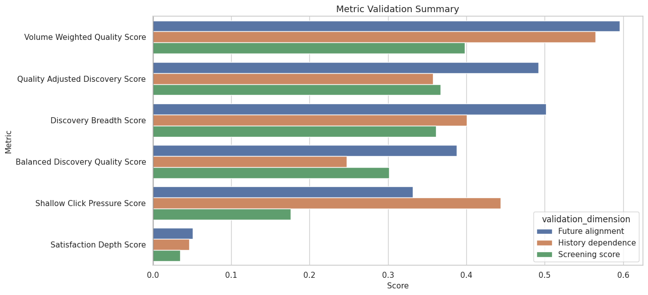

The visual summary is useful for portfolio communication because it shows the tradeoff in one place. A candidate metric is stronger when it has enough future signal without becoming just another activity-volume measure.

16. Select Metrics for Later Causal Notebooks

This cell chooses the metrics that will move forward. The choices preserve causal roles: an exposure-like metric for treatment, a satisfaction metric for mediation, a composite metric for product-level monitoring, and a guardrail for shallow engagement pressure.

selected_metrics = pd.DataFrame(
    [
        {
            "selected_for": "exposure_analysis",
            "metric": "discovery_breadth_score",
            "reason": "Purest discovery exposure score; does not use future outcomes or satisfaction depth as a defining component.",
        },
        {
            "selected_for": "mediator_analysis",
            "metric": "satisfaction_depth_score",
            "reason": "Aggregates several same-day quality signals and is appropriate as a mediator candidate.",
        },
        {
            "selected_for": "product_metric_monitoring",
            "metric": "quality_adjusted_discovery_score",
            "reason": "Requires both discovery breadth and satisfaction depth to be high, making it a useful composite quality metric.",
        },
        {
            "selected_for": "guardrail_monitoring",
            "metric": "shallow_click_pressure_score",
            "reason": "Flags high-volume days with low satisfaction, useful as a warning against click-only optimization.",
        },
    ]
)

selected_validation = selected_metrics.merge(
    validation_summary[
        [
            "metric",
            "future_alignment_score",
            "history_dependence_score",
            "screening_score",
            "top_minus_bottom_future_interactions",
        ]
    ],
    on="metric",
    how="left",
)

display(selected_validation.round(3))

	selected_for	metric	reason	future_alignment_score	history_dependence_score	screening_score	top_minus_bottom_future_interactions
0	exposure_analysis	discovery_breadth_score	Purest discovery exposure score; does not use future outcomes or satisfaction depth as a defining component.	0.502	0.401	0.361	368.238
1	mediator_analysis	satisfaction_depth_score	Aggregates several same-day quality signals and is appropriate as a mediator candidate.	0.051	0.046	0.035	-23.404
2	product_metric_monitoring	quality_adjusted_discovery_score	Requires both discovery breadth and satisfaction depth to be high, making it a useful composite quality metric.	0.492	0.357	0.367	349.624
3	guardrail_monitoring	shallow_click_pressure_score	Flags high-volume days with low satisfaction, useful as a warning against click-only optimization.	0.332	0.444	0.176	284.229

The selected set gives the next notebooks a clean structure: exposure first, mediator second, product composite third, guardrail alongside them. That keeps the causal story easy to follow instead of mixing every engineered score into every role.

17. Save Metric Artifacts

This cell writes the metric panel and validation outputs to disk. The next notebooks can now load one metric panel rather than rebuilding the score definitions. The registry and selection files make the metric choices auditable.

metric_panel.to_parquet(METRIC_PANEL_OUTPUT, index=False)
metric_registry.to_csv(METRIC_REGISTRY_OUTPUT, index=False)
validation_summary.to_csv(METRIC_VALIDATION_OUTPUT, index=False)
same_day_correlation.to_csv(METRIC_CORRELATION_OUTPUT)
metric_deciles.to_csv(METRIC_DECILE_OUTPUT, index=False)
selected_validation.to_csv(METRIC_SELECTION_OUTPUT, index=False)

# Mirror the most important tables inside the notebook writeup directory for easier export.
metric_registry.to_csv(TABLE_DIR / "metric_registry.csv", index=False)
validation_summary.to_csv(TABLE_DIR / "metric_validation_summary.csv", index=False)
metric_deciles.to_csv(TABLE_DIR / "metric_deciles.csv", index=False)
selected_validation.to_csv(TABLE_DIR / "selected_metrics.csv", index=False)

saved_outputs = pd.DataFrame(
    {
        "artifact": [
            "metric_panel",
            "metric_registry",
            "metric_validation_summary",
            "metric_correlation_matrix",
            "metric_decile_table",
            "selected_metrics",
        ],
        "path": [
            str(METRIC_PANEL_OUTPUT),
            str(METRIC_REGISTRY_OUTPUT),
            str(METRIC_VALIDATION_OUTPUT),
            str(METRIC_CORRELATION_OUTPUT),
            str(METRIC_DECILE_OUTPUT),
            str(METRIC_SELECTION_OUTPUT),
        ],
    }
)

display(saved_outputs)

	artifact	path
0	metric_panel	/home/apex/Documents/ranking_sys/data/processed/kuairec_discovery_quality_metric_panel.parquet
1	metric_registry	/home/apex/Documents/ranking_sys/data/processed/kuairec_discovery_quality_metric_registry.csv
2	metric_validation_summary	/home/apex/Documents/ranking_sys/data/processed/kuairec_discovery_quality_metric_validation.csv
3	metric_correlation_matrix	/home/apex/Documents/ranking_sys/data/processed/kuairec_discovery_quality_metric_correlations.csv
4	metric_decile_table	/home/apex/Documents/ranking_sys/data/processed/kuairec_discovery_quality_metric_deciles.csv
5	selected_metrics	/home/apex/Documents/ranking_sys/data/processed/kuairec_discovery_quality_selected_metrics.csv

The saved artifacts are the handoff point. The next notebook can focus on mediation estimands and assumptions because metric construction is now explicit, validated, and reproducible.

18. Notebook Takeaways

This notebook created a measurement layer for discovery quality. The main takeaways are:

• Discovery-quality measurement should separate exposure, mediator, composite, and guardrail roles.
• discovery_breadth_score is the cleanest exposure-like metric for later causal contrasts.
• satisfaction_depth_score is the main mediator candidate because it aggregates watch-quality signals without using future outcomes.
• quality_adjusted_discovery_score is useful as a product-facing metric, but it combines exposure and mediator information.
• Future outcomes validate the direction of the metrics, while history-dependence checks remind us why causal adjustment is still needed.

The natural next notebook is 03_mediation_estimands_and_assumptions.ipynb, where these metrics can be mapped to direct, indirect, and total effect estimands.