Discovery Quality Problem Setup and EDA

This notebook starts the discovery-quality mediation workflow using KuaiRec.

The causal problem is that short-term interaction metrics do not necessarily measure durable user value. A recommendation exposure can create immediate engagement but still fail to improve satisfaction or future activity. For discovery systems, this distinction matters because a metric such as CTR or interaction volume can reward curiosity, novelty, or low-friction behavior without proving that users were satisfied.

The workflow studies the pathway:

Exposure -> Immediate engagement -> Satisfaction -> Future engagement

This first notebook does not estimate mediation effects yet. It prepares the data and clarifies the measurement problem:

Dataset Field Guide

KuaiRec is stored locally as a zip file that contains another KuaiRec.zip archive. The main files used in this workflow are below.

small_matrix.csv and big_matrix.csv

These are user-video interaction matrices. small_matrix.csv is used here because it is large enough for realistic EDA but small enough to process quickly.

  • user_id: anonymized user identifier.
  • video_id: anonymized video identifier.
  • play_duration: watched time in milliseconds.
  • video_duration: video length in milliseconds.
  • time: interaction timestamp as a readable datetime string.
  • date: calendar date in YYYYMMDD form.
  • timestamp: Unix timestamp for the interaction.
  • watch_ratio: play_duration / video_duration. Values can exceed 1 when a user rewatches, loops, or spends longer than the nominal video duration.

user_features.csv

This file contains anonymized user profile and activity features.

  • user_id: anonymized user identifier.
  • user_active_degree: categorical user activity level.
  • is_lowactive_period: whether the user is in a low-activity period.
  • is_live_streamer: whether the user is marked as a live streamer.
  • is_video_author: whether the user has authored videos.
  • follow_user_num: count of followed users.
  • follow_user_num_range: binned follow count.
  • fans_user_num: count of fans.
  • fans_user_num_range: binned fan count.
  • friend_user_num: count of friends.
  • friend_user_num_range: binned friend count.
  • register_days: days since registration.
  • register_days_range: binned registration age.
  • onehot_feat0 through onehot_feat17: anonymized categorical or profile features encoded as integers. The raw feature meanings are not provided, so they should be used as controls rather than interpreted directly.

item_categories.csv

This file maps videos to category feature IDs.

  • video_id: anonymized video identifier.
  • feat: list-like category feature IDs for the video.

kuairec_caption_category.csv

This file provides richer video metadata.

  • video_id: anonymized video identifier.
  • manual_cover_text: text shown on the video cover when available.
  • caption: video caption text when available.
  • topic_tag: list-like topic tags.
  • first_level_category_id: broad category ID.
  • first_level_category_name: broad category name.
  • second_level_category_id: mid-level category ID.
  • second_level_category_name: mid-level category name.
  • third_level_category_id: fine category ID.
  • third_level_category_name: fine category name.

item_daily_features.csv

This file contains daily aggregate item metrics. It is useful for item-level popularity and platform-level context.

  • Identity and item state: video_id, date, author_id, video_type, upload_dt, upload_type, visible_status, video_duration, video_width, video_height, music_id, video_tag_id, video_tag_name.
  • Exposure and play counts: show_cnt, show_user_num, play_cnt, play_user_num, play_duration, complete_play_cnt, complete_play_user_num, valid_play_cnt, valid_play_user_num, long_time_play_cnt, long_time_play_user_num, short_time_play_cnt, short_time_play_user_num, play_progress.
  • Engagement actions: comment_stay_duration, like_cnt, like_user_num, click_like_cnt, double_click_cnt, cancel_like_cnt, cancel_like_user_num, comment_cnt, comment_user_num, direct_comment_cnt, reply_comment_cnt, delete_comment_cnt, delete_comment_user_num, comment_like_cnt, comment_like_user_num, follow_cnt, follow_user_num, cancel_follow_cnt, cancel_follow_user_num, share_cnt, share_user_num, download_cnt, download_user_num.
  • Negative or corrective feedback: report_cnt, report_user_num, reduce_similar_cnt, reduce_similar_user_num.
  • Collection actions: collect_cnt, collect_user_num, cancel_collect_cnt, cancel_collect_user_num.

Causal Measurement Setup

For this project, the first version of the mediation setup uses:

  • Treatment candidate: high discovery exposure on a user-day, measured by a high share of long-tail or new-category videos.
  • Immediate engagement mediator: valid play share or interaction intensity on the same day.
  • Satisfaction mediator: average watch ratio, high-watch share, or completion/rewatch share.
  • Future outcome: future 7-day interactions, active days, and play time.

The later mediation notebooks will formalize assumptions and estimate direct, indirect, and total effects.

1. Environment and Paths

This cell imports the libraries used for the setup notebook. It also finds the repository root by searching for the local KuaiRec zip file, then creates project-specific writeup folders for figures and tables.

from io import BytesIO
from pathlib import Path
from zipfile import ZipFile

import matplotlib.pyplot as plt
import numpy as np
import pandas as pd
import seaborn as sns
from IPython.display import display

sns.set_theme(style="whitegrid", context="notebook")
pd.set_option("display.max_columns", 120)
pd.set_option("display.max_rows", 100)
pd.set_option("display.float_format", lambda value: f"{value:,.4f}")

candidate_roots = [Path.cwd(), *Path.cwd().parents]
PROJECT_DIR = next(
    root for root in candidate_roots
    if (root / "data" / "Kuairec" / "18164998.zip").exists()
)

DATA_DIR = PROJECT_DIR / "data"
RAW_ZIP = DATA_DIR / "Kuairec" / "18164998.zip"
PROCESSED_DIR = DATA_DIR / "processed"
PROCESSED_DIR.mkdir(parents=True, exist_ok=True)

NOTEBOOK_DIR = PROJECT_DIR / "notebooks" / "discovery_quality_mediation"
WRITEUP_DIR = NOTEBOOK_DIR / "writeup"
FIGURE_DIR = WRITEUP_DIR / "figures"
TABLE_DIR = WRITEUP_DIR / "tables"
FIGURE_DIR.mkdir(parents=True, exist_ok=True)
TABLE_DIR.mkdir(parents=True, exist_ok=True)

RAW_ZIP.exists(), RAW_ZIP
(True, PosixPath('/home/apex/Documents/ranking_sys/data/Kuairec/18164998.zip'))

The path check should return True. The notebook will read from the local KuaiRec archive and save processed discovery-quality artifacts under data/processed.

2. Inspect the KuaiRec Archive

KuaiRec is distributed as an outer zip that contains a nested KuaiRec.zip. This cell lists the outer files and the nested files so the notebook documents exactly which local data assets are being used.

with ZipFile(RAW_ZIP) as outer_zip:
    outer_files = pd.DataFrame(
        [
            {
                "file": info.filename,
                "uncompressed_mb": info.file_size / 1_000_000,
                "compressed_mb": info.compress_size / 1_000_000,
            }
            for info in outer_zip.infolist()
            if not info.is_dir()
        ]
    )
    nested_bytes = outer_zip.read("KuaiRec.zip")

with ZipFile(BytesIO(nested_bytes)) as inner_zip:
    nested_files = pd.DataFrame(
        [
            {
                "file": info.filename,
                "uncompressed_mb": info.file_size / 1_000_000,
                "compressed_mb": info.compress_size / 1_000_000,
            }
            for info in inner_zip.infolist()
            if not info.is_dir()
        ]
    ).sort_values("uncompressed_mb", ascending=False)

display(outer_files)
display(nested_files)
file uncompressed_mb compressed_mb
0 KuaiRec.zip 431.9649 431.9649
1 kuairec_caption_category.csv 1.9646 1.9646
2 video_raw_categories_multi.csv 1.7245 1.7245
3 user_features_raw.csv 1.5416 1.5416
file uncompressed_mb compressed_mb
2 KuaiRec 2.0/data/big_matrix.csv 1,083.5212 292.5965
6 KuaiRec 2.0/data/small_matrix.csv 406.1558 119.1462
4 KuaiRec 2.0/data/item_daily_features.csv 85.8552 19.0098
5 KuaiRec 2.0/data/kuairec_caption_category.csv 1.9646 0.6010
8 KuaiRec 2.0/data/user_features.csv 0.7442 0.1223
1 KuaiRec 2.0/Statistics_KuaiRec.ipynb 0.3142 0.1893
9 KuaiRec 2.0/figs/KuaiRec.png 0.3002 0.2551
3 KuaiRec 2.0/data/item_categories.csv 0.1131 0.0315
0 KuaiRec 2.0/LICENSE 0.0201 0.0060
7 KuaiRec 2.0/data/social_network.csv 0.0069 0.0030
10 KuaiRec 2.0/figs/colab-badge.svg 0.0024 0.0011
11 KuaiRec 2.0/loaddata.py 0.0012 0.0004

The archive inspection shows why small_matrix.csv is the right starting point. It is a substantial interaction table, while big_matrix.csv is much larger. The metadata tables are small enough to load fully or with selected columns.

3. Load Metadata Tables

This cell loads user features, video category metadata, and selected daily item aggregate columns. These tables provide context for discovery-quality analysis: user controls, video categories, and item popularity signals.

with ZipFile(BytesIO(nested_bytes)) as inner_zip:
    with inner_zip.open("KuaiRec 2.0/data/user_features.csv") as file:
        user_features = pd.read_csv(file)
    with inner_zip.open("KuaiRec 2.0/data/item_categories.csv") as file:
        item_categories = pd.read_csv(file)
    caption_cols = [
        "video_id",
        "first_level_category_id",
        "first_level_category_name",
        "second_level_category_id",
        "second_level_category_name",
        "third_level_category_id",
        "third_level_category_name",
    ]
    with inner_zip.open("KuaiRec 2.0/data/kuairec_caption_category.csv") as file:
        caption_categories = pd.read_csv(
            file,
            usecols=caption_cols,
            engine="python",
            on_bad_lines="skip",
        )
    item_daily_cols = [
        "video_id",
        "date",
        "video_duration",
        "show_cnt",
        "show_user_num",
        "play_cnt",
        "play_user_num",
        "complete_play_cnt",
        "valid_play_cnt",
        "long_time_play_cnt",
        "short_time_play_cnt",
        "play_progress",
        "like_cnt",
        "comment_cnt",
        "follow_cnt",
        "share_cnt",
        "collect_cnt",
        "report_cnt",
        "reduce_similar_cnt",
        "video_tag_name",
    ]
    with inner_zip.open("KuaiRec 2.0/data/item_daily_features.csv") as file:
        item_daily = pd.read_csv(file, usecols=item_daily_cols)

for metadata_df in [user_features, item_categories, caption_categories, item_daily]:
    if "user_id" in metadata_df.columns:
        metadata_df["user_id"] = pd.to_numeric(metadata_df["user_id"], errors="coerce").astype("Int64")
    if "video_id" in metadata_df.columns:
        metadata_df["video_id"] = pd.to_numeric(metadata_df["video_id"], errors="coerce").astype("Int64")

item_categories = item_categories.dropna(subset=["video_id"]).copy()
caption_categories = caption_categories.dropna(subset=["video_id"]).copy()
item_daily = item_daily.dropna(subset=["video_id"]).copy()
item_categories["video_id"] = item_categories["video_id"].astype("int32")
caption_categories["video_id"] = caption_categories["video_id"].astype("int32")
item_daily["video_id"] = item_daily["video_id"].astype("int32")

metadata_summary = pd.DataFrame(
    {
        "table": ["user_features", "item_categories", "caption_categories", "item_daily_selected"],
        "rows": [len(user_features), len(item_categories), len(caption_categories), len(item_daily)],
        "columns": [user_features.shape[1], item_categories.shape[1], caption_categories.shape[1], item_daily.shape[1]],
        "unique_users": [user_features["user_id"].nunique(), np.nan, np.nan, np.nan],
        "unique_videos": [np.nan, item_categories["video_id"].nunique(), caption_categories["video_id"].nunique(), item_daily["video_id"].nunique()],
    }
)

display(metadata_summary)
display(user_features.head())
display(caption_categories.head())
table rows columns unique_users unique_videos
0 user_features 7176 31 7,176.0000 NaN
1 item_categories 10728 2 NaN 10,728.0000
2 caption_categories 10728 7 NaN 10,728.0000
3 item_daily_selected 343341 20 NaN 10,728.0000
user_id user_active_degree is_lowactive_period is_live_streamer is_video_author follow_user_num follow_user_num_range fans_user_num fans_user_num_range friend_user_num friend_user_num_range register_days register_days_range onehot_feat0 onehot_feat1 onehot_feat2 onehot_feat3 onehot_feat4 onehot_feat5 onehot_feat6 onehot_feat7 onehot_feat8 onehot_feat9 onehot_feat10 onehot_feat11 onehot_feat12 onehot_feat13 onehot_feat14 onehot_feat15 onehot_feat16 onehot_feat17
0 0 high_active 0 0 0 5 (0,10] 0 0 0 0 107 61-90 0 1 17 638 2.0000 0 1 6 184 6 3 0 0.0000 0.0000 0.0000 0.0000 0.0000 0.0000
1 1 full_active 0 0 0 386 (250,500] 4 [1,10) 2 [1,5) 327 181-365 0 3 25 1021 0.0000 0 1 6 186 6 2 0 0.0000 0.0000 0.0000 0.0000 0.0000 0.0000
2 2 full_active 0 0 0 27 (10,50] 0 0 0 0 116 91-180 0 6 8 402 0.0000 0 0 2 51 2 3 0 0.0000 0.0000 0.0000 0.0000 0.0000 0.0000
3 3 full_active 0 0 0 16 (10,50] 0 0 0 0 105 61-90 0 1 8 281 0.0000 0 0 34 251 3 2 0 0.0000 0.0000 0.0000 0.0000 0.0000 0.0000
4 4 full_active 0 0 0 122 (100,150] 4 [1,10) 0 0 225 181-365 0 1 8 316 1.0000 0 1 46 99 4 2 0 0.0000 0.0000 0.0000 0.0000 0.0000 0.0000
video_id first_level_category_id first_level_category_name second_level_category_id second_level_category_name third_level_category_id third_level_category_name
0 0 8.0000 颜值 673.0000 颜值随拍 -124.0000 UNKNOWN
1 1 27.0000 高新数码 -124.0000 UNKNOWN -124.0000 UNKNOWN
2 2 9.0000 喜剧 727.0000 搞笑互动 -124.0000 UNKNOWN
3 3 26.0000 摄影 686.0000 主题摄影 2,434.0000 景物摄影
4 4 5.0000 时尚 737.0000 营销售卖 2,596.0000 女装

The metadata tables give the controls and content context needed for mediation. User features help describe who is active. Category metadata lets us define new-category or diverse-discovery exposure. Item daily aggregates help define long-tail content more carefully than row counts alone.

4. Build a Deterministic Interaction Sample

This cell scans small_matrix.csv in chunks and keeps complete interaction histories for users whose user_id is divisible by a fixed modulus. Sampling complete users is better than sampling random rows because later mediation analysis needs user-day histories and future outcomes.

The scan also records full-file row counts, unique users, unique videos, and timestamp coverage.

USER_SAMPLE_MODULUS = 10
INTERACTION_CHUNK_ROWS = 750_000

interaction_dtypes = {
    "user_id": "int32",
    "video_id": "int32",
    "play_duration": "int32",
    "video_duration": "int32",
    "date": "float64",
    "timestamp": "float64",
    "watch_ratio": "float32",
}

sample_chunks = []
full_rows = 0
all_users = set()
all_videos = set()
timestamp_min = np.inf
timestamp_max = -np.inf

with ZipFile(BytesIO(nested_bytes)) as inner_zip:
    with inner_zip.open("KuaiRec 2.0/data/small_matrix.csv") as file:
        for chunk in pd.read_csv(file, chunksize=INTERACTION_CHUNK_ROWS, dtype=interaction_dtypes):
            full_rows += len(chunk)
            all_users.update(chunk["user_id"].unique().tolist())
            all_videos.update(chunk["video_id"].unique().tolist())
            timestamp_min = min(timestamp_min, chunk["timestamp"].min())
            timestamp_max = max(timestamp_max, chunk["timestamp"].max())

            sample = chunk.loc[chunk["user_id"] % USER_SAMPLE_MODULUS == 0].copy()
            if not sample.empty:
                sample_chunks.append(sample)

interactions = pd.concat(sample_chunks, ignore_index=True)

sample_summary = pd.DataFrame(
    {
        "metric": [
            "full_rows_scanned",
            "full_unique_users",
            "full_unique_videos",
            "full_timestamp_min",
            "full_timestamp_max",
            "sample_modulus",
            "sample_rows",
            "sample_unique_users",
            "sample_unique_videos",
        ],
        "value": [
            full_rows,
            len(all_users),
            len(all_videos),
            pd.to_datetime(timestamp_min, unit="s"),
            pd.to_datetime(timestamp_max, unit="s"),
            USER_SAMPLE_MODULUS,
            len(interactions),
            interactions["user_id"].nunique(),
            interactions["video_id"].nunique(),
        ],
    }
)

display(sample_summary)
display(interactions.head())
metric value
0 full_rows_scanned 4676570
1 full_unique_users 1411
2 full_unique_videos 3327
3 full_timestamp_min 2020-07-03 18:23:26.059999943
4 full_timestamp_max 2020-09-05 15:57:23.683000088
5 sample_modulus 10
6 sample_rows 440788
7 sample_unique_users 133
8 sample_unique_videos 3327
user_id video_id play_duration video_duration time date timestamp watch_ratio
0 120 5228 7174 9900 2020-07-05 07:01:50.19 20,200,705.0000 1,593,903,710.1900 0.7246
1 120 6788 4685 14934 2020-07-05 07:05:40.676 20,200,705.0000 1,593,903,940.6760 0.3137
2 120 8207 4923 13834 2020-07-05 07:39:22.913 20,200,705.0000 1,593,905,962.9130 0.3559
3 120 1936 3834 7100 2020-07-05 08:24:57.112 20,200,705.0000 1,593,908,697.1120 0.5400
4 120 5266 6110 7074 2020-07-05 08:34:43.594 20,200,705.0000 1,593,909,283.5940 0.8637

The sample keeps a meaningful number of users and interactions while remaining fast to work with. Because we sampled users rather than isolated rows, each sampled user can contribute a coherent daily sequence for future outcome construction.

5. Clean Interaction Time and Watch Signals

This cell turns raw interaction fields into analysis-ready variables. Watch ratio is capped for plotting and robust summaries, while the uncapped version is preserved. The notebook also creates first-pass proxies for immediate engagement and satisfaction.

interactions = interactions.copy()
interactions["event_time"] = pd.to_datetime(interactions["time"], errors="coerce")
interactions["event_date"] = pd.to_datetime(
    interactions["date"].round().astype("Int64").astype("string"),
    format="%Y%m%d",
    errors="coerce",
)
interactions["event_timestamp"] = pd.to_datetime(interactions["timestamp"], unit="s", errors="coerce")
interactions["play_duration_sec"] = interactions["play_duration"] / 1000
interactions["video_duration_sec"] = interactions["video_duration"] / 1000
interactions["watch_ratio_clean"] = interactions["watch_ratio"].replace([np.inf, -np.inf], np.nan)
interactions["watch_ratio_capped_5"] = interactions["watch_ratio_clean"].clip(lower=0, upper=5)
interactions["watch_ratio_capped_2"] = interactions["watch_ratio_clean"].clip(lower=0, upper=2)

interactions["played_proxy"] = (interactions["play_duration"] > 0).astype("int8")
interactions["valid_play_proxy"] = (
    (interactions["watch_ratio_clean"] >= 0.20) | (interactions["play_duration_sec"] >= 5)
).astype("int8")
interactions["high_satisfaction_proxy"] = (interactions["watch_ratio_clean"] >= 0.80).astype("int8")
interactions["complete_or_rewatch"] = (interactions["watch_ratio_clean"] >= 1.00).astype("int8")
interactions["short_abandon_proxy"] = (interactions["watch_ratio_clean"] < 0.20).astype("int8")
interactions["satisfaction_score_proxy"] = (
    0.50 * (interactions["watch_ratio_capped_2"] / 2)
    + 0.25 * interactions["valid_play_proxy"]
    + 0.25 * interactions["complete_or_rewatch"]
)

cleaning_summary = pd.DataFrame(
    {
        "metric": [
            "rows",
            "missing_event_time",
            "missing_event_date",
            "missing_watch_ratio",
            "played_proxy_rate",
            "valid_play_proxy_rate",
            "high_satisfaction_proxy_rate",
            "complete_or_rewatch_rate",
            "short_abandon_proxy_rate",
        ],
        "value": [
            len(interactions),
            interactions["event_time"].isna().sum(),
            interactions["event_date"].isna().sum(),
            interactions["watch_ratio_clean"].isna().sum(),
            interactions["played_proxy"].mean(),
            interactions["valid_play_proxy"].mean(),
            interactions["high_satisfaction_proxy"].mean(),
            interactions["complete_or_rewatch"].mean(),
            interactions["short_abandon_proxy"].mean(),
        ],
    }
)

display(cleaning_summary)
display(interactions.head())
metric value
0 rows 440,788.0000
1 missing_event_time 17,640.0000
2 missing_event_date 17,640.0000
3 missing_watch_ratio 0.0000
4 played_proxy_rate 0.9940
5 valid_play_proxy_rate 0.9376
6 high_satisfaction_proxy_rate 0.4562
7 complete_or_rewatch_rate 0.3102
8 short_abandon_proxy_rate 0.1026
user_id video_id play_duration video_duration time date timestamp watch_ratio event_time event_date event_timestamp play_duration_sec video_duration_sec watch_ratio_clean watch_ratio_capped_5 watch_ratio_capped_2 played_proxy valid_play_proxy high_satisfaction_proxy complete_or_rewatch short_abandon_proxy satisfaction_score_proxy
0 120 5228 7174 9900 2020-07-05 07:01:50.19 20,200,705.0000 1,593,903,710.1900 0.7246 2020-07-05 07:01:50.190 2020-07-05 2020-07-04 23:01:50.190000057 7.1740 9.9000 0.7246 0.7246 0.7246 1 1 0 0 0 0.4312
1 120 6788 4685 14934 2020-07-05 07:05:40.676 20,200,705.0000 1,593,903,940.6760 0.3137 2020-07-05 07:05:40.676 2020-07-05 2020-07-04 23:05:40.676000118 4.6850 14.9340 0.3137 0.3137 0.3137 1 1 0 0 0 0.3284
2 120 8207 4923 13834 2020-07-05 07:39:22.913 20,200,705.0000 1,593,905,962.9130 0.3559 2020-07-05 07:39:22.913 2020-07-05 2020-07-04 23:39:22.913000107 4.9230 13.8340 0.3559 0.3559 0.3559 1 1 0 0 0 0.3390
3 120 1936 3834 7100 2020-07-05 08:24:57.112 20,200,705.0000 1,593,908,697.1120 0.5400 2020-07-05 08:24:57.112 2020-07-05 2020-07-05 00:24:57.111999989 3.8340 7.1000 0.5400 0.5400 0.5400 1 1 0 0 0 0.3850
4 120 5266 6110 7074 2020-07-05 08:34:43.594 20,200,705.0000 1,593,909,283.5940 0.8637 2020-07-05 08:34:43.594 2020-07-05 2020-07-05 00:34:43.594000101 6.1100 7.0740 0.8637 0.8637 0.8637 1 1 1 0 0 0.4659

The proxy variables are not final causal estimands yet. They are measurement candidates. The later metric-construction notebook can decide which satisfaction proxy is most defensible, but this first notebook makes the available signals explicit.

6. Basic Interaction EDA

This cell summarizes the interaction sample. It focuses on watch time, video duration, watch ratio, and the proxy outcomes that could become mediators.

interaction_eda = interactions[
    [
        "play_duration_sec",
        "video_duration_sec",
        "watch_ratio_clean",
        "watch_ratio_capped_5",
        "valid_play_proxy",
        "high_satisfaction_proxy",
        "complete_or_rewatch",
        "satisfaction_score_proxy",
    ]
].describe(percentiles=[0.1, 0.25, 0.5, 0.75, 0.9, 0.99]).T

missing_rates = interactions.isna().mean().sort_values(ascending=False).rename("missing_rate")

display(interaction_eda)
display(missing_rates[missing_rates > 0])
count mean std min 10% 25% 50% 75% 90% 99% max
play_duration_sec 440,788.0000 8.6600 13.1076 0.0000 3.4970 5.4120 7.3940 9.6290 12.7040 36.0803 991.3850
video_duration_sec 440,788.0000 14.4871 20.4696 3.0670 6.2230 7.5230 9.6000 11.9340 21.8340 139.8770 315.0720
watch_ratio_clean 440,788.0000 0.9100 1.4719 0.0000 0.1952 0.4500 0.7474 1.1024 1.5516 3.9765 165.9865
watch_ratio_capped_5 440,788.0000 0.8679 0.6863 0.0000 0.1952 0.4500 0.7474 1.1024 1.5516 3.9765 5.0000
valid_play_proxy 440,788.0000 0.9376 0.2419 0.0000 1.0000 1.0000 1.0000 1.0000 1.0000 1.0000 1.0000
high_satisfaction_proxy 440,788.0000 0.4562 0.4981 0.0000 0.0000 0.0000 0.0000 1.0000 1.0000 1.0000 1.0000
complete_or_rewatch 440,788.0000 0.3102 0.4626 0.0000 0.0000 0.0000 0.0000 1.0000 1.0000 1.0000 1.0000
satisfaction_score_proxy 440,788.0000 0.5164 0.2541 0.0000 0.2971 0.3625 0.4368 0.7756 0.8879 1.0000 1.0000
time              0.0400
date              0.0400
event_timestamp   0.0400
event_date        0.0400
event_time        0.0400
timestamp         0.0400
Name: missing_rate, dtype: float64

The distribution table shows why watch ratio is useful but needs care. It can exceed 1 because of rewatches or loops, and extreme values can dominate averages. Capped versions are useful for plotting and robust summaries, while uncapped values remain available for diagnostics.

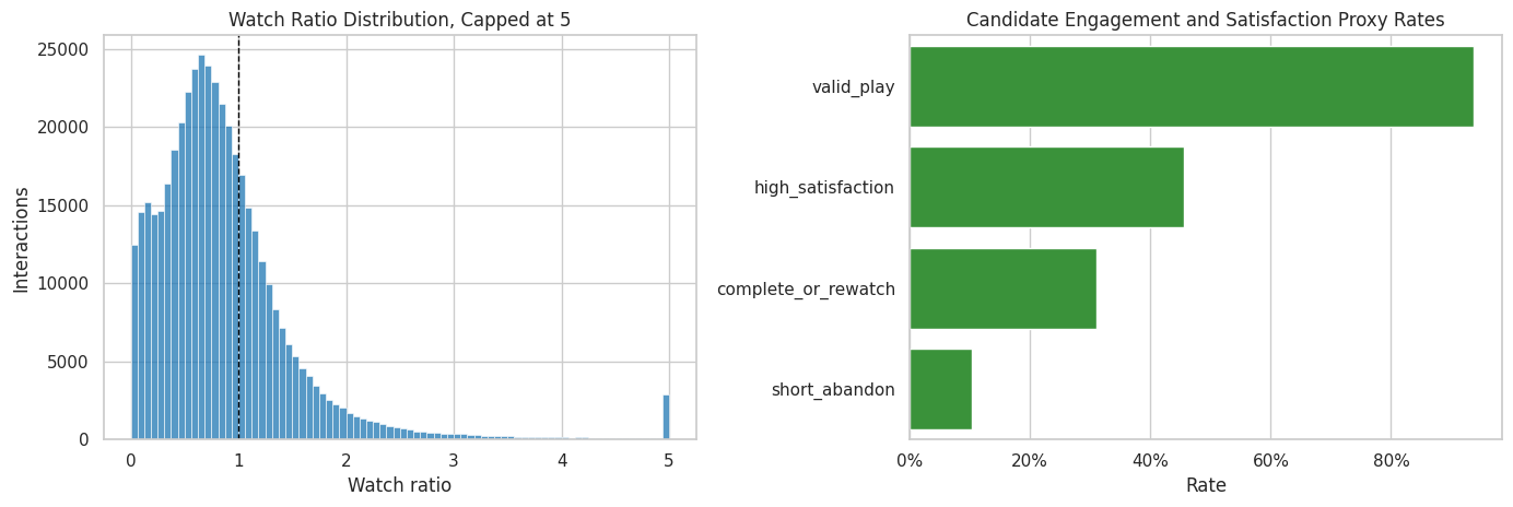
7. Plot Watch Ratio and Satisfaction Proxies

This cell visualizes the main same-day engagement and satisfaction signals. The watch-ratio plot is capped at 5 for readability; the proxy-rate plot summarizes binary measurement candidates.

fig, axes = plt.subplots(1, 2, figsize=(14, 4.8))

sns.histplot(interactions["watch_ratio_capped_5"], bins=80, ax=axes[0], color="tab:blue")
axes[0].axvline(1.0, color="black", linewidth=1, linestyle="--")
axes[0].set_title("Watch Ratio Distribution, Capped at 5")
axes[0].set_xlabel("Watch ratio")
axes[0].set_ylabel("Interactions")

proxy_rates = pd.DataFrame(
    {
        "proxy": ["valid_play", "high_satisfaction", "complete_or_rewatch", "short_abandon"],
        "rate": [
            interactions["valid_play_proxy"].mean(),
            interactions["high_satisfaction_proxy"].mean(),
            interactions["complete_or_rewatch"].mean(),
            interactions["short_abandon_proxy"].mean(),
        ],
    }
)
sns.barplot(data=proxy_rates, x="rate", y="proxy", ax=axes[1], color="tab:green")
axes[1].set_title("Candidate Engagement and Satisfaction Proxy Rates")
axes[1].set_xlabel("Rate")
axes[1].set_ylabel("")
axes[1].xaxis.set_major_formatter(lambda x, _: f"{x:.0%}")

plt.tight_layout()
fig.savefig(FIGURE_DIR / "01_watch_ratio_and_proxy_rates.png", dpi=160, bbox_inches="tight")
plt.show()

The plots show that satisfaction is richer than simple play occurrence. Most sampled rows are plays, so the more useful mediators are quality measures such as valid play, completion, high watch ratio, and abandonment.

8. Create Item Discovery Features

This cell builds item-level features from the interaction sample and metadata. The important feature is long_tail_item, a proxy for discovery-oriented content. Because KuaiRec’s small matrix can be close to dense across sampled users, sample interaction counts alone are not a good popularity measure here. We therefore define long-tail status from platform-level daily exposure counts (avg_show_cnt, with avg_play_cnt as a fallback), which better represents whether an item is broadly popular in the product environment.

item_sample_features = (
    interactions.groupby("video_id")
    .agg(
        sample_interactions=("user_id", "size"),
        sample_users=("user_id", "nunique"),
        sample_mean_watch_ratio=("watch_ratio_clean", "mean"),
        sample_high_satisfaction_rate=("high_satisfaction_proxy", "mean"),
        sample_complete_rate=("complete_or_rewatch", "mean"),
        sample_valid_play_rate=("valid_play_proxy", "mean"),
    )
    .reset_index()
)

item_daily_summary = (
    item_daily.groupby("video_id")
    .agg(
        daily_rows=("date", "size"),
        avg_show_cnt=("show_cnt", "mean"),
        avg_play_cnt=("play_cnt", "mean"),
        avg_play_progress=("play_progress", "mean"),
        avg_like_cnt=("like_cnt", "mean"),
        avg_share_cnt=("share_cnt", "mean"),
        avg_report_cnt=("report_cnt", "mean"),
        avg_reduce_similar_cnt=("reduce_similar_cnt", "mean"),
    )
    .reset_index()
)

item_features = (
    item_sample_features.merge(caption_categories, on="video_id", how="left")
    .merge(item_categories, on="video_id", how="left")
    .merge(item_daily_summary, on="video_id", how="left")
)

item_features["platform_popularity_score"] = (
    item_features["avg_show_cnt"]
    .combine_first(item_features["avg_play_cnt"])
    .combine_first(item_features["sample_interactions"].astype(float))
)
long_tail_threshold = item_features["platform_popularity_score"].quantile(0.40)
item_features["long_tail_item"] = (item_features["platform_popularity_score"] <= long_tail_threshold).astype("int8")
item_features["log_platform_popularity_score"] = np.log1p(item_features["platform_popularity_score"])
item_features["log_sample_interactions"] = np.log1p(item_features["sample_interactions"])
item_features["category_label"] = item_features["first_level_category_name"].fillna("unknown")

item_feature_summary = pd.DataFrame(
    {
        "metric": [
            "items_in_sample",
            "long_tail_threshold_platform_exposure",
            "long_tail_item_share",
            "categories_with_sampled_items",
            "items_missing_category",
            "sample_interaction_std",
            "platform_popularity_std",
        ],
        "value": [
            len(item_features),
            long_tail_threshold,
            item_features["long_tail_item"].mean(),
            item_features["category_label"].nunique(),
            item_features["first_level_category_name"].isna().sum(),
            item_features["sample_interactions"].std(),
            item_features["platform_popularity_score"].std(),
        ],
    }
)

display(item_feature_summary)
display(item_features.head())
metric value
0 items_in_sample 3,327.0000
1 long_tail_threshold_platform_exposure 65,221.2390
2 long_tail_item_share 0.4001
3 categories_with_sampled_items 39.0000
4 items_missing_category 2.0000
5 sample_interaction_std 1.6282
6 platform_popularity_std 584,997.9819
video_id sample_interactions sample_users sample_mean_watch_ratio sample_high_satisfaction_rate sample_complete_rate sample_valid_play_rate first_level_category_id first_level_category_name second_level_category_id second_level_category_name third_level_category_id third_level_category_name feat daily_rows avg_show_cnt avg_play_cnt avg_play_progress avg_like_cnt avg_share_cnt avg_report_cnt avg_reduce_similar_cnt platform_popularity_score long_tail_item log_platform_popularity_score log_sample_interactions category_label
0 103 133 133 0.8032 0.3835 0.2105 0.9173 12.0000 美食 153.0000 美食教程 1,460.0000 菜肴 [12] 63 109,310.6032 111,451.6190 0.5597 1,549.2698 99.9524 0.0000 36.4444 109,310.6032 0 11.6020 4.8978 美食
1 109 133 133 0.9869 0.6165 0.3835 0.9474 18.0000 汽车 716.0000 玩车 2,510.0000 机车族 [18, 5] 63 21,251.9206 14,303.1905 0.5789 629.0476 2.2540 0.0000 5.6667 21,251.9206 1 9.9642 4.8978 汽车
2 120 133 133 1.2237 0.7970 0.6767 0.9624 9.0000 喜剧 -124.0000 UNKNOWN -124.0000 UNKNOWN [9] 63 42,049.3492 41,847.3333 0.3802 2,683.6349 39.4762 0.0000 23.4286 42,049.3492 1 10.6466 4.8978 喜剧
3 122 133 133 0.8751 0.4662 0.2331 0.9474 9.0000 喜剧 548.0000 搞笑配音 -124.0000 UNKNOWN [9] 63 11,721.7302 11,728.4127 0.6210 169.3016 3.8730 0.0000 4.4444 11,721.7302 1 9.3693 4.8978 喜剧
4 128 133 133 0.7680 0.3383 0.1880 0.9323 12.0000 美食 292.0000 美食日常 1,461.0000 美食分享 [11, 12, 9] 63 436,061.3175 446,937.2698 0.7127 10,863.7937 62.5873 0.0635 235.0159 436,061.3175 0 12.9855 4.8978 美食

The long-tail definition now uses platform exposure rather than the dense sampled matrix. This matters because a causal setup needs treatment variation. If every active day had the same discovery exposure value, later mediation notebooks would have nothing meaningful to compare.

9. Enrich Interactions with Discovery Context

This cell joins item features back to each interaction and creates row-level discovery indicators. A row is a discovery candidate if the video is long-tail or if the video category is new to that user at the time of interaction.

interactions_enriched = interactions.merge(
    item_features[
        [
            "video_id",
            "category_label",
            "first_level_category_id",
            "second_level_category_id",
            "third_level_category_id",
            "sample_interactions",
            "sample_users",
            "sample_mean_watch_ratio",
            "sample_high_satisfaction_rate",
            "platform_popularity_score",
            "long_tail_item",
            "log_platform_popularity_score",
            "log_sample_interactions",
        ]
    ],
    on="video_id",
    how="left",
)

interactions_enriched = interactions_enriched.sort_values(["user_id", "event_time", "video_id"]).reset_index(drop=True)
interactions_enriched["user_category_seen_count"] = (
    interactions_enriched.groupby(["user_id", "category_label"]).cumcount()
)
interactions_enriched["new_category_for_user"] = (interactions_enriched["user_category_seen_count"] == 0).astype("int8")
interactions_enriched["discovery_candidate"] = (
    (interactions_enriched["long_tail_item"].fillna(0).eq(1))
    | (interactions_enriched["new_category_for_user"].eq(1))
).astype("int8")

interaction_discovery_summary = pd.DataFrame(
    {
        "metric": [
            "rows",
            "long_tail_interaction_share",
            "new_category_interaction_share",
            "discovery_candidate_share",
            "unique_categories",
        ],
        "value": [
            len(interactions_enriched),
            interactions_enriched["long_tail_item"].mean(),
            interactions_enriched["new_category_for_user"].mean(),
            interactions_enriched["discovery_candidate"].mean(),
            interactions_enriched["category_label"].nunique(),
        ],
    }
)

display(interaction_discovery_summary)
display(interactions_enriched.head())
metric value
0 rows 440,788.0000
1 long_tail_interaction_share 0.4005
2 new_category_interaction_share 0.0118
3 discovery_candidate_share 0.4080
4 unique_categories 39.0000
user_id video_id play_duration video_duration time date timestamp watch_ratio event_time event_date event_timestamp play_duration_sec video_duration_sec watch_ratio_clean watch_ratio_capped_5 watch_ratio_capped_2 played_proxy valid_play_proxy high_satisfaction_proxy complete_or_rewatch short_abandon_proxy satisfaction_score_proxy category_label first_level_category_id second_level_category_id third_level_category_id sample_interactions sample_users sample_mean_watch_ratio sample_high_satisfaction_rate platform_popularity_score long_tail_item log_platform_popularity_score log_sample_interactions user_category_seen_count new_category_for_user discovery_candidate
0 120 5228 7174 9900 2020-07-05 07:01:50.19 20,200,705.0000 1,593,903,710.1900 0.7246 2020-07-05 07:01:50.190 2020-07-05 2020-07-04 23:01:50.190000057 7.1740 9.9000 0.7246 0.7246 0.7246 1 1 0 0 0 0.4312 运动 7.0000 126.0000 1,056.0000 133 133 0.8021 0.4586 8,771.5818 1 9.0794 4.8978 0 1 1
1 120 6788 4685 14934 2020-07-05 07:05:40.676 20,200,705.0000 1,593,903,940.6760 0.3137 2020-07-05 07:05:40.676 2020-07-05 2020-07-04 23:05:40.676000118 4.6850 14.9340 0.3137 0.3137 0.3137 1 1 0 0 0 0.3284 二次元 20.0000 712.0000 2,491.0000 133 133 0.5268 0.0827 42,667.4444 1 10.6612 4.8978 0 1 1
2 120 8207 4923 13834 2020-07-05 07:39:22.913 20,200,705.0000 1,593,905,962.9130 0.3559 2020-07-05 07:39:22.913 2020-07-05 2020-07-04 23:39:22.913000107 4.9230 13.8340 0.3559 0.3559 0.3559 1 1 0 0 0 0.3390 喜剧 9.0000 136.0000 -124.0000 133 133 0.6196 0.2556 590,545.6984 0 13.2888 4.8978 0 1 1
3 120 1936 3834 7100 2020-07-05 08:24:57.112 20,200,705.0000 1,593,908,697.1120 0.5400 2020-07-05 08:24:57.112 2020-07-05 2020-07-05 00:24:57.111999989 3.8340 7.1000 0.5400 0.5400 0.5400 1 1 0 0 0 0.3850 运动 7.0000 126.0000 1,056.0000 132 132 1.2257 0.8030 13,711.4921 1 9.5261 4.8903 1 0 1
4 120 5266 6110 7074 2020-07-05 08:34:43.594 20,200,705.0000 1,593,909,283.5940 0.8637 2020-07-05 08:34:43.594 2020-07-05 2020-07-05 00:34:43.594000101 6.1100 7.0740 0.8637 0.8637 0.8637 1 1 1 0 0 0.4659 宠物 17.0000 -124.0000 -124.0000 133 133 1.2875 0.7519 34,720.4127 1 10.4551 4.8978 0 1 1

This row-level discovery marker is the bridge from EDA to causal design. It represents exposure to content that is either less popular or less familiar to the user. The later mediation notebook can test whether this exposure works through immediate engagement and satisfaction.

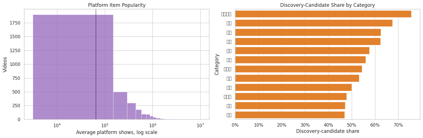
10. Plot Content Popularity and Discovery Exposure

This cell visualizes item popularity and discovery exposure. The popularity distribution shows whether there is a meaningful long tail, and the category plot shows where discovery-candidate interactions occur.

fig, axes = plt.subplots(1, 2, figsize=(15, 5))

sns.histplot(item_features["platform_popularity_score"], bins=70, ax=axes[0], color="tab:purple")
axes[0].set_xscale("log")
axes[0].axvline(long_tail_threshold, color="black", linewidth=1, linestyle="--")
axes[0].set_title("Platform Item Popularity")
axes[0].set_xlabel("Average platform shows, log scale")
axes[0].set_ylabel("Videos")

category_discovery = (
    interactions_enriched.groupby("category_label")
    .agg(rows=("video_id", "size"), discovery_share=("discovery_candidate", "mean"))
    .reset_index()
    .query("rows >= 500")
    .sort_values("discovery_share", ascending=False)
    .head(12)
)
sns.barplot(data=category_discovery, x="discovery_share", y="category_label", ax=axes[1], color="tab:orange")
axes[1].set_title("Discovery-Candidate Share by Category")
axes[1].set_xlabel("Discovery-candidate share")
axes[1].set_ylabel("Category")
axes[1].xaxis.set_major_formatter(lambda x, _: f"{x:.0%}")

plt.tight_layout()
fig.savefig(FIGURE_DIR / "02_popularity_and_discovery_exposure.png", dpi=160, bbox_inches="tight")
plt.show()

The plots confirm that discovery exposure has real variation. That is necessary for mediation: if every user-day had the same discovery exposure level, we could not study whether it changes engagement, satisfaction, or future activity.

11. Build a Balanced User-Day Panel

Mediation will be easier to define at the user-day level. This cell aggregates interactions into daily measures, then creates a balanced user-date panel so inactive future days are counted as zero activity rather than disappearing from the data.

daily_observed = (
    interactions_enriched.groupby(["user_id", "event_date"])
    .agg(
        interactions=("video_id", "size"),
        unique_videos=("video_id", "nunique"),
        unique_categories=("category_label", "nunique"),
        total_play_duration_sec=("play_duration_sec", "sum"),
        avg_play_duration_sec=("play_duration_sec", "mean"),
        avg_video_duration_sec=("video_duration_sec", "mean"),
        avg_watch_ratio=("watch_ratio_clean", "mean"),
        avg_watch_ratio_capped_2=("watch_ratio_capped_2", "mean"),
        valid_play_share=("valid_play_proxy", "mean"),
        high_satisfaction_share=("high_satisfaction_proxy", "mean"),
        complete_or_rewatch_share=("complete_or_rewatch", "mean"),
        short_abandon_share=("short_abandon_proxy", "mean"),
        avg_satisfaction_score=("satisfaction_score_proxy", "mean"),
        long_tail_share=("long_tail_item", "mean"),
        new_category_share=("new_category_for_user", "mean"),
        discovery_candidate_share=("discovery_candidate", "mean"),
    )
    .reset_index()
)

date_index = pd.date_range(interactions_enriched["event_date"].min(), interactions_enriched["event_date"].max(), freq="D")
user_index = np.sort(interactions_enriched["user_id"].unique())
balanced_index = pd.MultiIndex.from_product([user_index, date_index], names=["user_id", "event_date"])
user_day = balanced_index.to_frame(index=False).merge(daily_observed, on=["user_id", "event_date"], how="left")

count_cols = ["interactions", "unique_videos", "unique_categories", "total_play_duration_sec"]
share_cols = [
    "avg_play_duration_sec",
    "avg_video_duration_sec",
    "avg_watch_ratio",
    "avg_watch_ratio_capped_2",
    "valid_play_share",
    "high_satisfaction_share",
    "complete_or_rewatch_share",
    "short_abandon_share",
    "avg_satisfaction_score",
    "long_tail_share",
    "new_category_share",
    "discovery_candidate_share",
]
for col in count_cols + share_cols:
    user_day[col] = user_day[col].fillna(0)

user_day["active_day"] = (user_day["interactions"] > 0).astype("int8")
user_day["calendar_day_index"] = (user_day["event_date"] - user_day["event_date"].min()).dt.days
user_day = user_day.sort_values(["user_id", "event_date"]).reset_index(drop=True)

panel_summary = pd.DataFrame(
    {
        "metric": [
            "users",
            "calendar_days",
            "panel_rows",
            "active_day_rate",
            "mean_interactions_on_active_days",
            "mean_discovery_share_on_active_days",
        ],
        "value": [
            user_day["user_id"].nunique(),
            user_day["event_date"].nunique(),
            len(user_day),
            user_day["active_day"].mean(),
            user_day.loc[user_day["active_day"].eq(1), "interactions"].mean(),
            user_day.loc[user_day["active_day"].eq(1), "discovery_candidate_share"].mean(),
        ],
    }
)

display(panel_summary)
display(user_day.head())
metric value
0 users 133.0000
1 calendar_days 63.0000
2 panel_rows 8,379.0000
3 active_day_rate 0.9785
4 mean_interactions_on_active_days 51.6097
5 mean_discovery_share_on_active_days 0.3644
user_id event_date interactions unique_videos unique_categories total_play_duration_sec avg_play_duration_sec avg_video_duration_sec avg_watch_ratio avg_watch_ratio_capped_2 valid_play_share high_satisfaction_share complete_or_rewatch_share short_abandon_share avg_satisfaction_score long_tail_share new_category_share discovery_candidate_share active_day calendar_day_index
0 120 2020-07-05 32.0000 32.0000 16.0000 163.9700 5.1241 11.9891 0.5813 0.5813 0.9375 0.1562 0.0938 0.0625 0.4031 0.4062 0.5000 0.6875 1 0
1 120 2020-07-06 20.0000 20.0000 15.0000 130.9860 6.5493 13.4448 0.6965 0.6837 0.9500 0.3500 0.2000 0.1500 0.4584 0.3500 0.2500 0.4500 1 1
2 120 2020-07-07 16.0000 16.0000 10.0000 100.9200 6.3075 10.1208 0.6580 0.6580 1.0000 0.1875 0.0625 0.0000 0.4301 0.2500 0.3125 0.4375 1 2
3 120 2020-07-08 37.0000 37.0000 23.0000 222.7200 6.0195 21.1131 0.5842 0.5639 0.8919 0.2162 0.0541 0.2703 0.3775 0.3514 0.1351 0.4324 1 3
4 120 2020-07-09 34.0000 34.0000 14.0000 230.6110 6.7827 11.9327 0.6982 0.6982 1.0000 0.3235 0.2059 0.0294 0.4760 0.3824 0.0000 0.3824 1 4

The balanced panel is the core data structure for this project. It preserves inactive days, which matters for future engagement outcomes. It also summarizes discovery exposure and satisfaction on the same user-day.

12. Define Future Outcomes and History Controls

This cell creates future outcomes and lagged history controls. Later mediation models should adjust for prior user behavior because users with different histories may receive different exposure and have different future engagement.

def future_sum_by_user(frame, column, horizon):
    pieces = []
    grouped = frame.groupby("user_id", sort=False)[column]
    total = pd.Series(0.0, index=frame.index)
    for step in range(1, horizon + 1):
        total = total + grouped.shift(-step).fillna(0)
    return total

for col in ["active_day", "interactions", "total_play_duration_sec"]:
    user_day[f"lead_1_{col}"] = user_day.groupby("user_id")[col].shift(-1).fillna(0)
    user_day[f"future_3day_{col}"] = future_sum_by_user(user_day, col, 3)
    user_day[f"future_7day_{col}"] = future_sum_by_user(user_day, col, 7)

for col in [
    "active_day",
    "interactions",
    "total_play_duration_sec",
    "avg_watch_ratio_capped_2",
    "valid_play_share",
    "high_satisfaction_share",
    "discovery_candidate_share",
]:
    user_day[f"lag_1_{col}"] = user_day.groupby("user_id")[col].shift(1).fillna(0)
    user_day[f"prior_3day_{col}"] = (
        user_day.groupby("user_id")[col]
        .rolling(window=3, min_periods=1)
        .sum()
        .reset_index(level=0, drop=True)
        .groupby(user_day["user_id"])
        .shift(1)
        .fillna(0)
    )

future_summary = user_day[
    [
        "future_7day_active_day",
        "future_7day_interactions",
        "future_7day_total_play_duration_sec",
        "lag_1_interactions",
        "prior_3day_interactions",
    ]
].describe(percentiles=[0.25, 0.5, 0.75, 0.9]).T

display(future_summary)
count mean std min 25% 50% 75% 90% max
future_7day_active_day 8,379.0000 6.4157 1.5444 0.0000 7.0000 7.0000 7.0000 7.0000 7.0000
future_7day_interactions 8,379.0000 338.3823 182.2699 0.0000 202.0000 364.0000 470.0000 561.0000 899.0000
future_7day_total_play_duration_sec 8,379.0000 2,926.6982 1,698.1722 0.0000 1,726.1070 2,953.5820 4,037.2785 5,032.7692 10,442.1170
lag_1_interactions 8,379.0000 50.4739 32.3121 0.0000 27.0000 47.0000 69.0000 93.0000 293.0000
prior_3day_interactions 8,379.0000 151.1738 79.6062 0.0000 92.0000 149.0000 203.0000 254.0000 497.0000

The future outcomes provide the retention side of the mediation pathway. The lagged variables are not causal results; they are adjustment candidates that help later models compare similar user-days.

13. Define Treatment, Mediators, and Outcome Candidates

This cell creates first-pass variables for the mediation analysis. The treatment is high discovery exposure on an active day. The mediators are same-day engagement quality and satisfaction. The outcome is future 7-day engagement.

active_days = user_day.query("active_day == 1").copy()
discovery_threshold = active_days["discovery_candidate_share"].median()
long_tail_threshold_day = active_days["long_tail_share"].median()

user_day["treatment_high_discovery_exposure"] = (
    (user_day["active_day"].eq(1))
    & (user_day["discovery_candidate_share"] >= discovery_threshold)
).astype("int8")
user_day["treatment_high_long_tail_exposure"] = (
    (user_day["active_day"].eq(1))
    & (user_day["long_tail_share"] >= long_tail_threshold_day)
).astype("int8")

user_day["mediator_valid_play_share"] = user_day["valid_play_share"]
user_day["mediator_high_satisfaction_share"] = user_day["high_satisfaction_share"]
user_day["mediator_avg_satisfaction_score"] = user_day["avg_satisfaction_score"]
user_day["outcome_future_7day_interactions"] = user_day["future_7day_interactions"]
user_day["outcome_future_7day_active_days"] = user_day["future_7day_active_day"]
user_day["outcome_future_7day_play_hours"] = user_day["future_7day_total_play_duration_sec"] / 3600

mediation_panel = user_day.query("active_day == 1").copy()
mediation_panel = mediation_panel.merge(
    user_features,
    on="user_id",
    how="left",
)

candidate_summary = pd.DataFrame(
    [
        {
            "role": "treatment",
            "variable": "treatment_high_discovery_exposure",
            "mean": mediation_panel["treatment_high_discovery_exposure"].mean(),
            "description": "Active user-day has discovery-candidate share at or above the active-day median, where discovery combines platform long-tail status and first category exposure.",
        },
        {
            "role": "treatment_alt",
            "variable": "treatment_high_long_tail_exposure",
            "mean": mediation_panel["treatment_high_long_tail_exposure"].mean(),
            "description": "Active user-day has long-tail share at or above the active-day median.",
        },
        {
            "role": "mediator_engagement",
            "variable": "mediator_valid_play_share",
            "mean": mediation_panel["mediator_valid_play_share"].mean(),
            "description": "Share of interactions that look like valid plays.",
        },
        {
            "role": "mediator_satisfaction",
            "variable": "mediator_high_satisfaction_share",
            "mean": mediation_panel["mediator_high_satisfaction_share"].mean(),
            "description": "Share of interactions with watch ratio at least 0.8.",
        },
        {
            "role": "outcome",
            "variable": "outcome_future_7day_interactions",
            "mean": mediation_panel["outcome_future_7day_interactions"].mean(),
            "description": "Future 7-day interaction count after the current day.",
        },
        {
            "role": "outcome_alt",
            "variable": "outcome_future_7day_active_days",
            "mean": mediation_panel["outcome_future_7day_active_days"].mean(),
            "description": "Future 7-day active-day count after the current day.",
        },
    ]
)

display(candidate_summary)
display(mediation_panel.head())
role variable mean description
0 treatment treatment_high_discovery_exposure 0.5015 Active user-day has discovery-candidate share ...
1 treatment_alt treatment_high_long_tail_exposure 0.5001 Active user-day has long-tail share at or abov...
2 mediator_engagement mediator_valid_play_share 0.9394 Share of interactions that look like valid plays.
3 mediator_satisfaction mediator_high_satisfaction_share 0.4686 Share of interactions with watch ratio at leas...
4 outcome outcome_future_7day_interactions 340.6945 Future 7-day interaction count after the curre...
5 outcome_alt outcome_future_7day_active_days 6.4664 Future 7-day active-day count after the curren...
user_id event_date interactions unique_videos unique_categories total_play_duration_sec avg_play_duration_sec avg_video_duration_sec avg_watch_ratio avg_watch_ratio_capped_2 valid_play_share high_satisfaction_share complete_or_rewatch_share short_abandon_share avg_satisfaction_score long_tail_share new_category_share discovery_candidate_share active_day calendar_day_index lead_1_active_day future_3day_active_day future_7day_active_day lead_1_interactions future_3day_interactions future_7day_interactions lead_1_total_play_duration_sec future_3day_total_play_duration_sec future_7day_total_play_duration_sec lag_1_active_day prior_3day_active_day lag_1_interactions prior_3day_interactions lag_1_total_play_duration_sec prior_3day_total_play_duration_sec lag_1_avg_watch_ratio_capped_2 prior_3day_avg_watch_ratio_capped_2 lag_1_valid_play_share prior_3day_valid_play_share lag_1_high_satisfaction_share prior_3day_high_satisfaction_share lag_1_discovery_candidate_share prior_3day_discovery_candidate_share treatment_high_discovery_exposure treatment_high_long_tail_exposure mediator_valid_play_share mediator_high_satisfaction_share mediator_avg_satisfaction_score outcome_future_7day_interactions outcome_future_7day_active_days outcome_future_7day_play_hours user_active_degree is_lowactive_period is_live_streamer is_video_author follow_user_num follow_user_num_range fans_user_num fans_user_num_range friend_user_num friend_user_num_range register_days register_days_range onehot_feat0 onehot_feat1 onehot_feat2 onehot_feat3 onehot_feat4 onehot_feat5 onehot_feat6 onehot_feat7 onehot_feat8 onehot_feat9 onehot_feat10 onehot_feat11 onehot_feat12 onehot_feat13 onehot_feat14 onehot_feat15 onehot_feat16 onehot_feat17
0 120 2020-07-05 32.0000 32.0000 16.0000 163.9700 5.1241 11.9891 0.5813 0.5813 0.9375 0.1562 0.0938 0.0625 0.4031 0.4062 0.5000 0.6875 1 0 1.0000 3.0000 7.0000 20.0000 73.0000 316.0000 130.9860 454.6260 1,945.6300 0.0000 0.0000 0.0000 0.0000 0.0000 0.0000 0.0000 0.0000 0.0000 0.0000 0.0000 0.0000 0.0000 0.0000 1 1 0.9375 0.1562 0.4031 316.0000 7.0000 0.5405 full_active 0 0 0 7 (0,10] 3 [1,10) 0 0 224 181-365 0 1 24 876 1.0000 0 1 4 98 6 0 0 0.0000 0.0000 0.0000 0.0000 0.0000 0.0000
1 120 2020-07-06 20.0000 20.0000 15.0000 130.9860 6.5493 13.4448 0.6965 0.6837 0.9500 0.3500 0.2000 0.1500 0.4584 0.3500 0.2500 0.4500 1 1 1.0000 3.0000 7.0000 16.0000 87.0000 345.0000 100.9200 554.2510 2,111.7460 1.0000 1.0000 32.0000 32.0000 163.9700 163.9700 0.5813 0.5813 0.9375 0.9375 0.1562 0.1562 0.6875 0.6875 1 0 0.9500 0.3500 0.4584 345.0000 7.0000 0.5866 full_active 0 0 0 7 (0,10] 3 [1,10) 0 0 224 181-365 0 1 24 876 1.0000 0 1 4 98 6 0 0 0.0000 0.0000 0.0000 0.0000 0.0000 0.0000
2 120 2020-07-07 16.0000 16.0000 10.0000 100.9200 6.3075 10.1208 0.6580 0.6580 1.0000 0.1875 0.0625 0.0000 0.4301 0.2500 0.3125 0.4375 1 2 1.0000 3.0000 7.0000 37.0000 128.0000 393.0000 222.7200 789.3200 2,417.3040 1.0000 2.0000 20.0000 52.0000 130.9860 294.9560 0.6837 1.2650 0.9500 1.8875 0.3500 0.5062 0.4500 1.1375 1 0 1.0000 0.1875 0.4301 393.0000 7.0000 0.6715 full_active 0 0 0 7 (0,10] 3 [1,10) 0 0 224 181-365 0 1 24 876 1.0000 0 1 4 98 6 0 0 0.0000 0.0000 0.0000 0.0000 0.0000 0.0000
3 120 2020-07-08 37.0000 37.0000 23.0000 222.7200 6.0195 21.1131 0.5842 0.5639 0.8919 0.2162 0.0541 0.2703 0.3775 0.3514 0.1351 0.4324 1 3 1.0000 3.0000 7.0000 34.0000 144.0000 436.0000 230.6110 894.1200 2,725.9950 1.0000 3.0000 16.0000 68.0000 100.9200 395.8760 0.6580 1.9230 1.0000 2.8875 0.1875 0.6937 0.4375 1.5750 1 0 0.8919 0.2162 0.3775 436.0000 7.0000 0.7572 full_active 0 0 0 7 (0,10] 3 [1,10) 0 0 224 181-365 0 1 24 876 1.0000 0 1 4 98 6 0 0 0.0000 0.0000 0.0000 0.0000 0.0000 0.0000
4 120 2020-07-09 34.0000 34.0000 14.0000 230.6110 6.7827 11.9327 0.6982 0.6982 1.0000 0.3235 0.2059 0.0294 0.4760 0.3824 0.0000 0.3824 1 4 1.0000 3.0000 7.0000 57.0000 209.0000 448.0000 335.9890 1,260.3930 2,809.6920 1.0000 3.0000 37.0000 73.0000 222.7200 454.6260 0.5639 1.9056 0.8919 2.8419 0.2162 0.7537 0.4324 1.3199 0 1 1.0000 0.3235 0.4760 448.0000 7.0000 0.7805 full_active 0 0 0 7 (0,10] 3 [1,10) 0 0 224 181-365 0 1 24 876 1.0000 0 1 4 98 6 0 0 0.0000 0.0000 0.0000 0.0000 0.0000 0.0000

This table is the first explicit mediation setup. It does not prove causality yet. It defines a plausible treatment, mediators, and future outcomes so the next notebook can validate and refine the metric choices.

14. Compare Same-Day Metrics by Discovery Exposure

This cell compares mediators and future outcomes between high-discovery and lower-discovery active days. These are raw differences, not adjusted causal effects, but they help us see whether the variables have meaningful variation.

comparison_metrics = [
    "interactions",
    "valid_play_share",
    "high_satisfaction_share",
    "complete_or_rewatch_share",
    "avg_satisfaction_score",
    "outcome_future_7day_interactions",
    "outcome_future_7day_active_days",
    "outcome_future_7day_play_hours",
    "lag_1_interactions",
    "prior_3day_interactions",
]

raw_means = mediation_panel.groupby("treatment_high_discovery_exposure")[comparison_metrics].mean()
for arm in [0, 1]:
    if arm not in raw_means.index:
        raw_means.loc[arm] = np.nan
raw_means = raw_means.sort_index()

raw_comparison = pd.DataFrame(
    {
        "metric": comparison_metrics,
        "lower_discovery_days": raw_means.loc[0, comparison_metrics].to_numpy(),
        "high_discovery_days": raw_means.loc[1, comparison_metrics].to_numpy(),
    }
)
raw_comparison["high_minus_lower"] = raw_comparison["high_discovery_days"] - raw_comparison["lower_discovery_days"]

display(raw_comparison)
metric lower_discovery_days high_discovery_days high_minus_lower
0 interactions 39.6538 63.4929 23.8392
1 valid_play_share 0.9377 0.9411 0.0033
2 high_satisfaction_share 0.4538 0.4834 0.0296
3 complete_or_rewatch_share 0.3138 0.3324 0.0185
4 avg_satisfaction_score 0.5187 0.5295 0.0108
5 outcome_future_7day_interactions 247.8894 432.9353 185.0459
6 outcome_future_7day_active_days 6.0595 6.8709 0.8114
7 outcome_future_7day_play_hours 0.6040 1.0326 0.4286
8 lag_1_interactions 41.1461 60.8570 19.7109
9 prior_3day_interactions 126.5388 178.4667 51.9279

Raw differences are useful for orientation. If high-discovery days also have very different prior activity, later mediation models need adjustment. The next notebooks should not interpret these simple differences as causal effects.

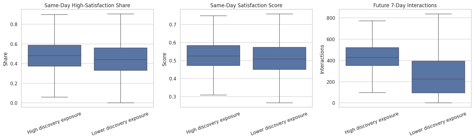
15. Plot Treatment, Mediators, and Future Outcome Relationships

This cell creates a compact visual summary of how discovery exposure relates to same-day satisfaction and future engagement. It is meant as EDA, not causal evidence.

plot_df = mediation_panel.copy()
plot_df["discovery_group"] = plot_df["treatment_high_discovery_exposure"].map(
    {0: "Lower discovery exposure", 1: "High discovery exposure"}
)

fig, axes = plt.subplots(1, 3, figsize=(16, 4.8))

sns.boxplot(
    data=plot_df,
    x="discovery_group",
    y="mediator_high_satisfaction_share",
    ax=axes[0],
    showfliers=False,
)
axes[0].set_title("Same-Day High-Satisfaction Share")
axes[0].set_xlabel("")
axes[0].set_ylabel("Share")
axes[0].tick_params(axis="x", rotation=20)

sns.boxplot(
    data=plot_df,
    x="discovery_group",
    y="mediator_avg_satisfaction_score",
    ax=axes[1],
    showfliers=False,
)
axes[1].set_title("Same-Day Satisfaction Score")
axes[1].set_xlabel("")
axes[1].set_ylabel("Score")
axes[1].tick_params(axis="x", rotation=20)

sns.boxplot(
    data=plot_df,
    x="discovery_group",
    y="outcome_future_7day_interactions",
    ax=axes[2],
    showfliers=False,
)
axes[2].set_title("Future 7-Day Interactions")
axes[2].set_xlabel("")
axes[2].set_ylabel("Interactions")
axes[2].tick_params(axis="x", rotation=20)

plt.tight_layout()
fig.savefig(FIGURE_DIR / "03_discovery_mediator_outcome_relationships.png", dpi=160, bbox_inches="tight")
plt.show()

The plots show the measurement pathway in one place: discovery exposure, satisfaction-like mediators, and future engagement. This helps check whether the later mediation analysis will be numerically meaningful.

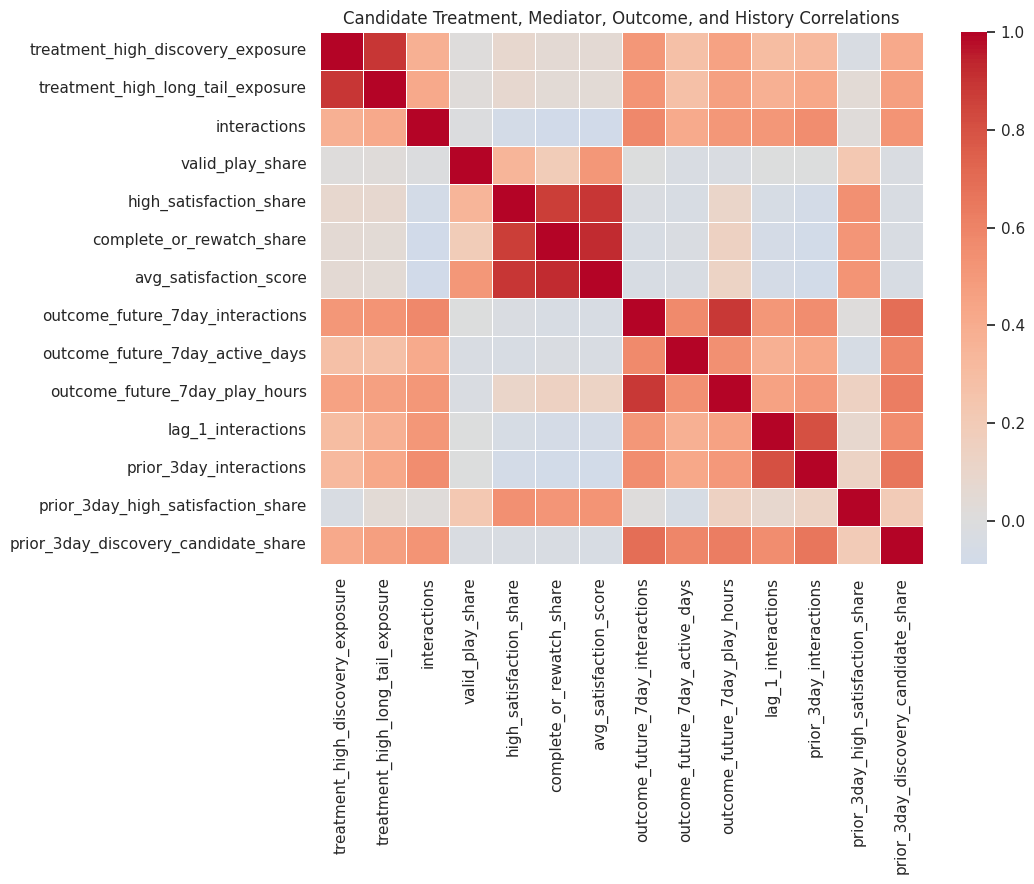
16. Correlation Map for Candidate Variables

This cell computes correlations among treatment, mediators, outcomes, and prior-history controls. Correlation is not causation, but it is a useful diagnostic for variable redundancy and expected model behavior.

correlation_columns = [
    "treatment_high_discovery_exposure",
    "treatment_high_long_tail_exposure",
    "interactions",
    "valid_play_share",
    "high_satisfaction_share",
    "complete_or_rewatch_share",
    "avg_satisfaction_score",
    "outcome_future_7day_interactions",
    "outcome_future_7day_active_days",
    "outcome_future_7day_play_hours",
    "lag_1_interactions",
    "prior_3day_interactions",
    "prior_3day_high_satisfaction_share",
    "prior_3day_discovery_candidate_share",
]

correlation_matrix = mediation_panel[correlation_columns].corr()

fig, ax = plt.subplots(figsize=(11, 9))
sns.heatmap(correlation_matrix, cmap="coolwarm", center=0, linewidths=0.5, ax=ax)
ax.set_title("Candidate Treatment, Mediator, Outcome, and History Correlations")
plt.tight_layout()
fig.savefig(FIGURE_DIR / "04_candidate_variable_correlation_map.png", dpi=160, bbox_inches="tight")
plt.show()

display(correlation_matrix.round(3))

treatment_high_discovery_exposure treatment_high_long_tail_exposure interactions valid_play_share high_satisfaction_share complete_or_rewatch_share avg_satisfaction_score outcome_future_7day_interactions outcome_future_7day_active_days outcome_future_7day_play_hours lag_1_interactions prior_3day_interactions prior_3day_high_satisfaction_share prior_3day_discovery_candidate_share
treatment_high_discovery_exposure 1.0000 0.8900 0.3760 0.0170 0.0840 0.0540 0.0530 0.5130 0.2790 0.4580 0.3070 0.3280 -0.0340 0.4170
treatment_high_long_tail_exposure 0.8900 1.0000 0.4210 0.0190 0.0740 0.0410 0.0410 0.5260 0.2800 0.4680 0.3760 0.4260 0.0450 0.4750
interactions 0.3760 0.4210 1.0000 -0.0140 -0.0700 -0.0880 -0.0860 0.5800 0.4120 0.5150 0.5150 0.5590 0.0270 0.5290
valid_play_share 0.0170 0.0190 -0.0140 1.0000 0.3460 0.1920 0.5130 -0.0050 -0.0300 -0.0240 -0.0070 -0.0050 0.2240 -0.0260
high_satisfaction_share 0.0840 0.0740 -0.0700 0.3460 1.0000 0.8670 0.8920 -0.0270 -0.0380 0.1110 -0.0530 -0.0690 0.5380 -0.0300
complete_or_rewatch_share 0.0540 0.0410 -0.0880 0.1920 0.8670 1.0000 0.9230 -0.0460 -0.0230 0.1420 -0.0630 -0.0820 0.5160 -0.0320
avg_satisfaction_score 0.0530 0.0410 -0.0860 0.5130 0.8920 0.9230 1.0000 -0.0400 -0.0320 0.1310 -0.0620 -0.0800 0.5280 -0.0460
outcome_future_7day_interactions 0.5130 0.5260 0.5800 -0.0050 -0.0270 -0.0460 -0.0400 1.0000 0.5770 0.8810 0.5110 0.5610 0.0110 0.6930
outcome_future_7day_active_days 0.2790 0.2800 0.4120 -0.0300 -0.0380 -0.0230 -0.0320 0.5770 1.0000 0.5380 0.3780 0.4230 -0.0500 0.5830
outcome_future_7day_play_hours 0.4580 0.4680 0.5150 -0.0240 0.1110 0.1420 0.1310 0.8810 0.5380 1.0000 0.4580 0.5040 0.1440 0.6270
lag_1_interactions 0.3070 0.3760 0.5150 -0.0070 -0.0530 -0.0630 -0.0620 0.5110 0.3780 0.4580 1.0000 0.8060 0.0810 0.5560
prior_3day_interactions 0.3280 0.4260 0.5590 -0.0050 -0.0690 -0.0820 -0.0800 0.5610 0.4230 0.5040 0.8060 1.0000 0.1260 0.6590
prior_3day_high_satisfaction_share -0.0340 0.0450 0.0270 0.2240 0.5380 0.5160 0.5280 0.0110 -0.0500 0.1440 0.0810 0.1260 1.0000 0.2030
prior_3day_discovery_candidate_share 0.4170 0.4750 0.5290 -0.0260 -0.0300 -0.0320 -0.0460 0.6930 0.5830 0.6270 0.5560 0.6590 0.2030 1.0000

The correlation map helps identify which variables are likely to act as confounders or redundant mediators. In particular, prior activity variables should be treated carefully because they can predict both current exposure and future outcomes.

17. Readiness Checks for Mediation Analysis

This cell summarizes whether the constructed panel is ready for the next notebook. It checks sample size, treatment variation, mediator variation, future-outcome variation, and missingness in key variables.

key_variables = [
    "treatment_high_discovery_exposure",
    "mediator_valid_play_share",
    "mediator_high_satisfaction_share",
    "mediator_avg_satisfaction_score",
    "outcome_future_7day_interactions",
    "outcome_future_7day_active_days",
    "lag_1_interactions",
    "prior_3day_interactions",
]

readiness_checks = pd.DataFrame(
    [
        {
            "check": "active_user_days",
            "value": len(mediation_panel),
            "notes": "Rows available for active-day mediation setup.",
        },
        {
            "check": "sampled_users",
            "value": mediation_panel["user_id"].nunique(),
            "notes": "Users represented in the mediation panel.",
        },
        {
            "check": "treatment_rate",
            "value": mediation_panel["treatment_high_discovery_exposure"].mean(),
            "notes": "Should be neither near 0 nor near 1.",
        },
        {
            "check": "mediator_satisfaction_std",
            "value": mediation_panel["mediator_high_satisfaction_share"].std(),
            "notes": "Mediator must vary across user-days.",
        },
        {
            "check": "future_7day_interactions_std",
            "value": mediation_panel["outcome_future_7day_interactions"].std(),
            "notes": "Outcome must vary across user-days.",
        },
        {
            "check": "max_key_variable_missing_rate",
            "value": mediation_panel[key_variables].isna().mean().max(),
            "notes": "Key variables should be complete or nearly complete.",
        },
    ]
)

display(readiness_checks)
check value notes
0 active_user_days 8,199.0000 Rows available for active-day mediation setup.
1 sampled_users 133.0000 Users represented in the mediation panel.
2 treatment_rate 0.5015 Should be neither near 0 nor near 1.
3 mediator_satisfaction_std 0.1766 Mediator must vary across user-days.
4 future_7day_interactions_std 180.3633 Outcome must vary across user-days.
5 max_key_variable_missing_rate 0.0000 Key variables should be complete or nearly com...

The readiness checks should support moving to metric construction. If treatment, mediators, or future outcomes lacked variation, mediation would be weak. Here the panel has enough structure for the next notebook to compare candidate discovery-quality metrics.

18. Save Processed Discovery-Quality Artifacts

This cell saves the processed interaction sample, item features, user-day panel, mediation panel, candidate variable summary, and readiness checks. Later notebooks can load these directly.

INTERACTIONS_OUTPUT = PROCESSED_DIR / "kuairec_discovery_quality_interactions_sample.parquet"
ITEM_FEATURES_OUTPUT = PROCESSED_DIR / "kuairec_discovery_quality_item_features.parquet"
USER_DAY_OUTPUT = PROCESSED_DIR / "kuairec_discovery_quality_user_day_panel.parquet"
MEDIATION_PANEL_OUTPUT = PROCESSED_DIR / "kuairec_discovery_quality_mediation_panel.parquet"
CANDIDATE_SUMMARY_OUTPUT = PROCESSED_DIR / "kuairec_discovery_quality_candidate_variables.csv"
READINESS_OUTPUT = PROCESSED_DIR / "kuairec_discovery_quality_readiness.csv"
RAW_COMPARISON_OUTPUT = PROCESSED_DIR / "kuairec_discovery_quality_raw_comparison.csv"

interactions_enriched.to_parquet(INTERACTIONS_OUTPUT, index=False)
item_features.to_parquet(ITEM_FEATURES_OUTPUT, index=False)
user_day.to_parquet(USER_DAY_OUTPUT, index=False)
mediation_panel.to_parquet(MEDIATION_PANEL_OUTPUT, index=False)
candidate_summary.to_csv(CANDIDATE_SUMMARY_OUTPUT, index=False)
readiness_checks.to_csv(READINESS_OUTPUT, index=False)
raw_comparison.to_csv(RAW_COMPARISON_OUTPUT, index=False)

saved_outputs = pd.DataFrame(
    {
        "artifact": [
            "interactions_sample",
            "item_features",
            "user_day_panel",
            "mediation_panel",
            "candidate_variable_summary",
            "readiness_checks",
            "raw_discovery_comparison",
        ],
        "path": [
            str(INTERACTIONS_OUTPUT),
            str(ITEM_FEATURES_OUTPUT),
            str(USER_DAY_OUTPUT),
            str(MEDIATION_PANEL_OUTPUT),
            str(CANDIDATE_SUMMARY_OUTPUT),
            str(READINESS_OUTPUT),
            str(RAW_COMPARISON_OUTPUT),
        ],
    }
)

display(saved_outputs)
artifact path
0 interactions_sample /home/apex/Documents/ranking_sys/data/processe...
1 item_features /home/apex/Documents/ranking_sys/data/processe...
2 user_day_panel /home/apex/Documents/ranking_sys/data/processe...
3 mediation_panel /home/apex/Documents/ranking_sys/data/processe...
4 candidate_variable_summary /home/apex/Documents/ranking_sys/data/processe...
5 readiness_checks /home/apex/Documents/ranking_sys/data/processe...
6 raw_discovery_comparison /home/apex/Documents/ranking_sys/data/processe...

These saved files are the handoff to the next notebook. The mediation panel is the most important artifact because it contains treatment candidates, mediator candidates, future outcomes, and history controls in one user-day table.

19. Notebook Takeaways

This notebook established the data foundation for discovery-quality mediation:

  • KuaiRec is a strong fit because it has watch duration, watch ratio, user features, item categories, and sequential user activity.
  • The project should not treat play occurrence alone as satisfaction. Watch ratio, completion/rewatch, high-satisfaction share, and abandonment are richer signals.
  • Discovery exposure can be represented by long-tail content and new-category content, then aggregated to a user-day treatment candidate.
  • Future 7-day engagement can be measured with interactions, active days, and play hours.
  • The next notebook should validate and refine the discovery-quality metric before formal mediation estimation.