This notebook closes the interference and spillover workflow.
The analysis studied a recommendation setting where items compete for limited slate attention. A lower-ranked focal movie was randomly promoted in simulated MovieLens slates. That promotion helped the focal item, but it also shifted visibility away from other movies. The central question was not only whether the promoted item gained clicks, but whether the full slate gained value after accounting for displaced competitors.
This final notebook packages the work into portfolio-ready artifacts:
final effect tables,
direct, indirect, and total effect summaries,
spillover sensitivity checks,
advanced-model targeting results,
limitations and recommendations,
markdown writeups and resume bullets.
The main conclusion is that promoted-item gains alone are misleading under interference. In this simulation, the focal item gained engagement, but competitor losses more than offset that gain, producing a negative total slate effect.
1. Environment and Paths
This cell imports the tools used for final reporting and sets up the writeup folders. The notebook searches upward for the processed interference outputs so it can run from either JupyterLab or command-line execution.
from pathlib import Pathimport matplotlib.pyplot as pltimport numpy as npimport pandas as pdimport seaborn as snsfrom IPython.display import displaysns.set_theme(style="whitegrid", context="notebook")pd.set_option("display.max_columns", 140)pd.set_option("display.max_rows", 120)pd.set_option("display.float_format", lambda value: f"{value:,.4f}")candidate_roots = [Path.cwd(), *Path.cwd().parents]PROJECT_DIR =next( root for root in candidate_rootsif (root /"data"/"processed"/"movielens_interference_observed_effects.csv").exists())PROCESSED_DIR = PROJECT_DIR /"data"/"processed"NOTEBOOK_DIR = PROJECT_DIR /"notebooks"/"interference_spillover_effects"WRITEUP_DIR = NOTEBOOK_DIR /"writeup"FIGURE_DIR = WRITEUP_DIR /"figures"TABLE_DIR = WRITEUP_DIR /"tables"FIGURE_DIR.mkdir(parents=True, exist_ok=True)TABLE_DIR.mkdir(parents=True, exist_ok=True)WRITEUP_DIR, FIGURE_DIR, TABLE_DIR
The writeup folders keep final report artifacts colocated with the notebooks. Figures go into writeup/figures, tables go into writeup/tables, and markdown summaries go into the writeup root.
2. Load Final Inputs
This cell loads all outputs needed for the final report. These tables come from the earlier notebooks: setup, exposure mapping, randomized estimation, decomposition, and advanced modeling.
paths = {"setup_readiness": PROCESSED_DIR /"movielens_interference_setup_readiness.csv","exposure_readiness": PROCESSED_DIR /"movielens_interference_exposure_readiness.csv","observed_effects": PROCESSED_DIR /"movielens_interference_observed_effects.csv","direct_indirect_total": PROCESSED_DIR /"movielens_interference_direct_indirect_total_effects.csv","additivity_checks": PROCESSED_DIR /"movielens_interference_additivity_checks.csv","spillover_sensitivity": PROCESSED_DIR /"movielens_interference_spillover_definition_sensitivity.csv","product_summary": PROCESSED_DIR /"movielens_interference_product_summary.csv","recommendations": PROCESSED_DIR /"movielens_interference_decomposition_recommendations.csv","advanced_metrics": PROCESSED_DIR /"movielens_interference_advanced_model_metrics.csv","advanced_aipw": PROCESSED_DIR /"movielens_interference_advanced_aipw_estimates.csv","advanced_policy": PROCESSED_DIR /"movielens_interference_advanced_policy_targeting.csv","advanced_takeaways": PROCESSED_DIR /"movielens_interference_advanced_takeaways.csv","advanced_heterogeneity": PROCESSED_DIR /"movielens_interference_advanced_heterogeneity.csv","cluster_risk": PROCESSED_DIR /"movielens_interference_cluster_risk.csv","position_risk": PROCESSED_DIR /"movielens_interference_position_risk.csv",}loaded = {name: pd.read_csv(path) for name, path in paths.items()}load_index = pd.DataFrame( {"artifact": list(paths.keys()),"path": [str(path) for path in paths.values()],"rows": [len(loaded[name]) for name in paths], })display(load_index)
artifact
path
rows
0
setup_readiness
/home/apex/Documents/ranking_sys/data/processe...
7
1
exposure_readiness
/home/apex/Documents/ranking_sys/data/processe...
8
2
observed_effects
/home/apex/Documents/ranking_sys/data/processe...
5
3
direct_indirect_total
/home/apex/Documents/ranking_sys/data/processe...
12
4
additivity_checks
/home/apex/Documents/ranking_sys/data/processe...
3
5
spillover_sensitivity
/home/apex/Documents/ranking_sys/data/processe...
5
6
product_summary
/home/apex/Documents/ranking_sys/data/processe...
5
7
recommendations
/home/apex/Documents/ranking_sys/data/processe...
4
8
advanced_metrics
/home/apex/Documents/ranking_sys/data/processe...
4
9
advanced_aipw
/home/apex/Documents/ranking_sys/data/processe...
3
10
advanced_policy
/home/apex/Documents/ranking_sys/data/processe...
5
11
advanced_takeaways
/home/apex/Documents/ranking_sys/data/processe...
4
12
advanced_heterogeneity
/home/apex/Documents/ranking_sys/data/processe...
21
13
cluster_risk
/home/apex/Documents/ranking_sys/data/processe...
5
14
position_risk
/home/apex/Documents/ranking_sys/data/processe...
3
The load index is a compact inventory of the full workflow. If a final table looks surprising, this index makes it easy to trace which upstream notebook produced the source data.
3. Build the Final Main Effects Table
This cell cleans the main randomized-estimator output. It converts estimates to report-friendly units and keeps the key quantities: direct focal effect, spillover effects, and total slate effect.
observed_effects = loaded["observed_effects"].copy()final_effects = observed_effects[ ["contrast","outcome","estimate","cluster_se","ci_95_lower","ci_95_upper","treated_mean","control_mean","treated_n","control_n","clusters", ]].copy()final_effects["estimate_per_1000"] = final_effects["estimate"] *1000final_effects["ci_95_lower_per_1000"] = final_effects["ci_95_lower"] *1000final_effects["ci_95_upper_per_1000"] = final_effects["ci_95_upper"] *1000final_effects["report_note"] = np.select( [ final_effects["contrast"].eq("Direct focal item"), final_effects["contrast"].str.contains("spillover", case=False, na=False), final_effects["contrast"].eq("Total slate"), ], ["Promoted focal item gain.","Competitor or non-focal item displacement.","Net slate-level value after direct and spillover effects.", ], default="Supporting contrast.",)final_effects_output = TABLE_DIR /"final_main_effects.csv"final_effects.to_csv(final_effects_output, index=False)display(final_effects)
contrast
outcome
estimate
cluster_se
ci_95_lower
ci_95_upper
treated_mean
control_mean
treated_n
control_n
clusters
estimate_per_1000
ci_95_lower_per_1000
ci_95_upper_per_1000
report_note
0
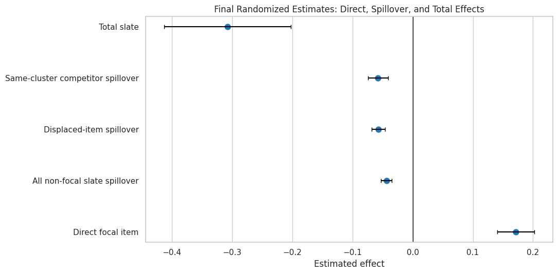
Direct focal item
Observed simulated click
0.1716
0.0157
0.1409
0.2023
0.3435
0.1719
1505
1495
3000
171.6152
140.9221
202.3083
Promoted focal item gain.
1
Same-cluster competitor spillover
Observed simulated click
-0.0577
0.0084
-0.0743
-0.0412
0.1522
0.2100
4309
4139
2456
-57.7146
-74.2530
-41.1761
Competitor or non-focal item displacement.
2
Displaced-item spillover
Observed simulated click
-0.0568
0.0057
-0.0679
-0.0457
0.1818
0.2386
11277
11133
3000
-56.7841
-67.8706
-45.6975
Competitor or non-focal item displacement.
3
All non-focal slate spillover
Observed simulated click
-0.0436
0.0046
-0.0526
-0.0346
0.1705
0.2141
16555
16445
3000
-43.5851
-52.6154
-34.5549
Competitor or non-focal item displacement.
4
Total slate
Observed total simulated clicks
-0.3078
0.0538
-0.4132
-0.2024
2.2193
2.5271
1505
1495
3000
-307.8212
-413.2036
-202.4388
Net slate-level value after direct and spillov...
This is the core result table. The focal item gains clicks, but the spillover rows are negative and the total slate effect is negative. That is the central evidence that item-level reporting would overstate product value.
4. Plot the Final Main Effects
This figure turns the main effects table into a clean final-report chart. It uses the original units for each contrast: item-level click-rate differences for item rows and total simulated clicks for the slate-level row.
The chart makes the contrast visible in one glance. The direct focal effect is positive, but every spillover contrast is negative and the net slate effect is negative. That is the practical signal that attention was reallocated rather than expanded.
5. Final Direct, Indirect, and Total Decomposition
This cell extracts the observed-click decomposition from the formal decomposition notebook. The table reports effects per promoted slate and per 1,000 promoted slates so the numbers can be used directly in a written summary.
decomposition = loaded["direct_indirect_total"].copy()observed_decomposition = decomposition.query("outcome_type == 'observed_clicks'").copy()observed_decomposition["component_label"] = observed_decomposition["effect_family"] +": "+ observed_decomposition["component"]component_order = ["Direct: Focal item","Indirect: Same-cluster competitors","Indirect: Other competitors","Total: Full slate",]observed_decomposition["component_order"] = observed_decomposition["component_label"].map( {label: i for i, label inenumerate(component_order)})observed_decomposition = observed_decomposition.sort_values("component_order")observed_decomposition_output = TABLE_DIR /"final_direct_indirect_total_decomposition.csv"observed_decomposition.to_csv(observed_decomposition_output, index=False)display(observed_decomposition[ ["effect_family","component","estimate_per_slate","ci_95_lower","ci_95_upper","estimate_per_1000_promoted_slates","ci_95_lower_per_1000","ci_95_upper_per_1000", ]])
effect_family
component
estimate_per_slate
ci_95_lower
ci_95_upper
estimate_per_1000_promoted_slates
ci_95_lower_per_1000
ci_95_upper_per_1000
0
Direct
Focal item
0.1716
0.1409
0.2023
171.6152
140.8990
202.3315
1
Indirect
Same-cluster competitors
-0.1454
-0.2015
-0.0892
-145.3905
-201.5497
-89.2313
2
Indirect
Other competitors
-0.3340
-0.4260
-0.2421
-334.0459
-425.9571
-242.1347
3
Total
Full slate
-0.3078
-0.4132
-0.2025
-307.8212
-413.1899
-202.4525
This decomposition is the most important final-report table. It shows the accounting: the direct focal gain is positive, but same-cluster and other-competitor losses combine into a larger negative indirect effect, so the full slate loses value.
6. Plot the Final Decomposition
This figure shows the same decomposition in clicks per 1,000 promoted slates. Positive bars are gains, negative bars are losses, and the total bar summarizes the net product effect.
fig, ax = plt.subplots(figsize=(11, 5.5))colors = ["tab:green"if value >=0else"tab:red"for value in observed_decomposition["estimate_per_1000_promoted_slates"]]sns.barplot( data=observed_decomposition, x="estimate_per_1000_promoted_slates", y="component_label", order=component_order, hue="component_label", palette=dict(zip(observed_decomposition["component_label"], colors)), legend=False, ax=ax,)for y_pos, (_, row) inenumerate(observed_decomposition.reset_index(drop=True).iterrows()): ax.errorbar( x=row["estimate_per_1000_promoted_slates"], y=y_pos, xerr=[ [row["estimate_per_1000_promoted_slates"] - row["ci_95_lower_per_1000"]], [row["ci_95_upper_per_1000"] - row["estimate_per_1000_promoted_slates"]], ], fmt="none", color="black", capsize=3, )ax.axvline(0, color="black", linewidth=1)ax.set_title("Final Decomposition per 1,000 Promoted Slates")ax.set_xlabel("Change in simulated clicks per 1,000 promoted slates")ax.set_ylabel("")plt.tight_layout()decomposition_figure = FIGURE_DIR /"26_final_direct_indirect_total_decomposition.png"fig.savefig(decomposition_figure, dpi=160, bbox_inches="tight")plt.show()
The figure is the clearest final visual for the project. It shows why the promoted item’s gain is not sufficient for product decision-making: the competitors lose more than the focal item gains.
7. Sensitivity Across Spillover Definitions
This cell packages the spillover sensitivity analysis. The goal is to check whether the spillover conclusion depends on one narrow definition of competition.
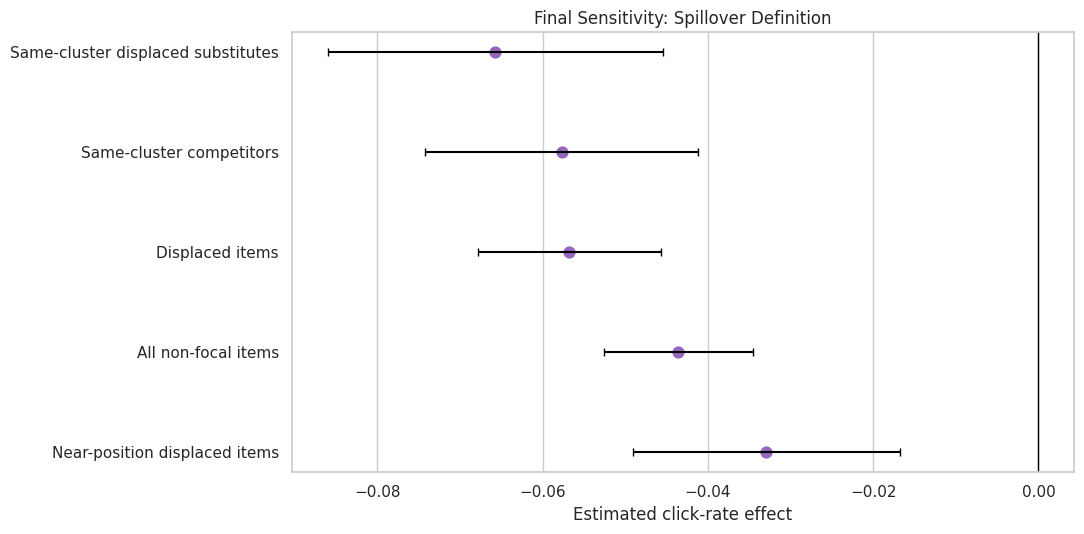
Every tested spillover definition is negative in this simulation. That makes the displacement conclusion stronger: it is not just an artifact of using one particular competitor definition.
8. Plot Spillover Sensitivity
This figure compares spillover definitions with confidence intervals. It helps show which competitor definitions are broad and which are stricter.
The sensitivity figure supports a cautious but clear claim: under several plausible definitions of competitor exposure, spillover effects are negative. That gives the final recommendation more weight.
9. Advanced Modeling Summary
This cell packages the advanced modeling results: outcome-model metrics, model-assisted AIPW estimates, counterfactual targeting, and the final takeaways. These results show that flexible models can help target safer promotions, but they do not overturn the randomized finding.
The advanced-model story is nuanced. XGBoost had the best held-out prediction performance, and the model-assisted AIPW estimate closely matched the randomized estimator. Targeting reduced harm mainly by promoting fewer slates, which reinforces the product lesson: promotions should be gated by expected net slate value.
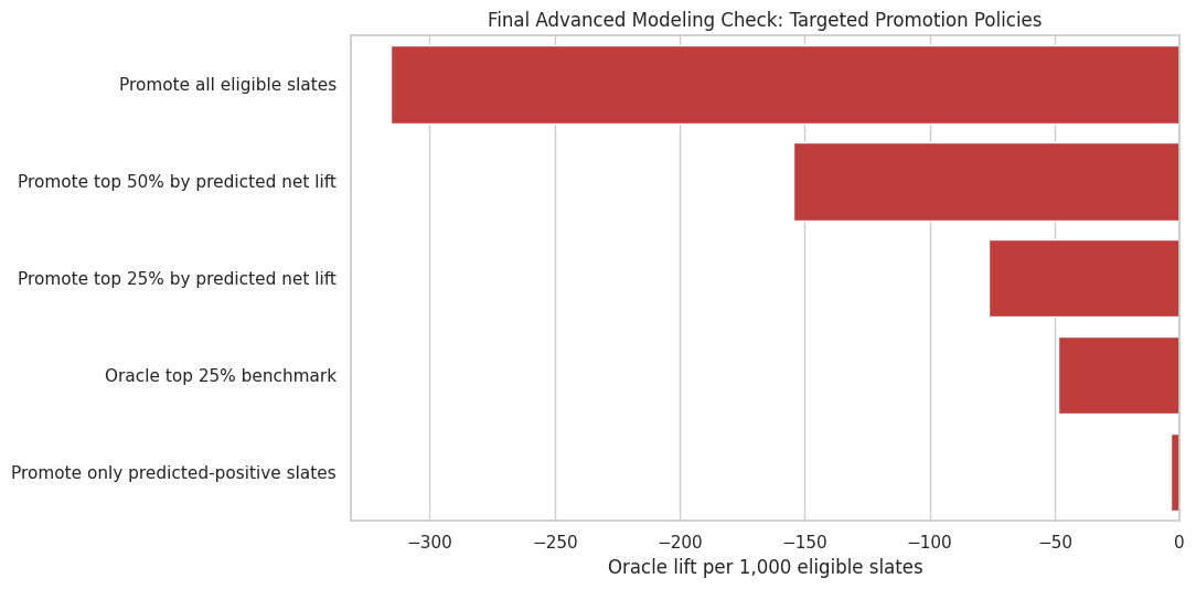
10. Plot Advanced Policy Targeting
This figure compares policy rules using oracle expected lift per 1,000 eligible slates. It rewards policies for selecting better slates but also accounts for how many slates they promote.
policy_plot = advanced_policy.sort_values("oracle_lift_per_1000_eligible_slates").copy()fig, ax = plt.subplots(figsize=(11, 5.5))colors = ["tab:green"if value >=0else"tab:red"for value in policy_plot["oracle_lift_per_1000_eligible_slates"]]sns.barplot( data=policy_plot, x="oracle_lift_per_1000_eligible_slates", y="policy", hue="policy", palette=dict(zip(policy_plot["policy"], colors)), legend=False, ax=ax,)ax.axvline(0, color="black", linewidth=1)ax.set_title("Final Advanced Modeling Check: Targeted Promotion Policies")ax.set_xlabel("Oracle lift per 1,000 eligible slates")ax.set_ylabel("")plt.tight_layout()policy_figure = FIGURE_DIR /"28_final_policy_targeting.png"fig.savefig(policy_figure, dpi=160, bbox_inches="tight")plt.show()
The targeting figure shows that model-based selection can reduce harm compared with promoting every eligible slate. It also shows that the simulation contains few broadly positive promotion opportunities, so restraint is part of the recommended policy.
11. Limitations Table
This cell writes a limitations table. The project is methodologically useful, but the final report should be honest about the fact that MovieLens ratings are not real exposure logs and the promotion process is simulated.
limitations = pd.DataFrame( [ {"limitation": "MovieLens contains ratings, not true recommendation impressions.","impact": "The analysis demonstrates an interference workflow but does not estimate real production promotion effects.","mitigation": "Use real slate impression logs or run a randomized slate experiment when available.", }, {"limitation": "Promotion assignment and outcomes are simulated.","impact": "The numerical estimates reflect the assumed data-generating process.","mitigation": "Treat the results as a methodology demonstration and validate with online experiments.", }, {"limitation": "Genres are coarse substitute clusters.","impact": "Some substitutes may be missed and some same-genre items may not actually compete.","mitigation": "Use learned item embeddings, co-watch patterns, or richer metadata for production analysis.", }, {"limitation": "Only one promotion design is simulated.","impact": "Different promotion probabilities, slate sizes, or ranking policies could change the net effect.","mitigation": "Run sensitivity analyses over assignment rules and promotion intensities.", }, {"limitation": "Advanced models are evaluated against simulated oracle lift.","impact": "Policy targeting results depend on the simulated outcome mechanism.","mitigation": "Use randomized or valid off-policy evaluation before deploying targeted promotion rules.", }, ])limitations_output = TABLE_DIR /"final_limitations.csv"limitations.to_csv(limitations_output, index=False)display(limitations)
limitation
impact
mitigation
0
MovieLens contains ratings, not true recommend...
The analysis demonstrates an interference work...
Use real slate impression logs or run a random...
1
Promotion assignment and outcomes are simulated.
The numerical estimates reflect the assumed da...
Treat the results as a methodology demonstrati...
2
Genres are coarse substitute clusters.
Some substitutes may be missed and some same-g...
Use learned item embeddings, co-watch patterns...
3
Only one promotion design is simulated.
Different promotion probabilities, slate sizes...
Run sensitivity analyses over assignment rules...
4
Advanced models are evaluated against simulate...
Policy targeting results depend on the simulat...
Use randomized or valid off-policy evaluation ...
The limitations make the final report more credible. They separate the transferable causal workflow from the specific numeric simulation results, which should not be presented as real-world platform lift.
12. Final Recommendations
This cell combines the earlier decomposition recommendations with final-report wording. The recommendations are framed as decision rules for recommendation systems where items compete for attention.
recommendations = loaded["recommendations"].copy()final_recommendations = pd.concat( [ recommendations, pd.DataFrame( [ {"decision_area": "Experiment design","recommendation": "Randomize at the slate, cluster, or market level when interference is plausible.","evidence": "Item-level treatment assignment can miss displacement across neighboring items.", }, {"decision_area": "Advanced targeting","recommendation": "Use ML targeting only after validating net slate value against a randomized or off-policy benchmark.","evidence": "The model-assisted AIPW estimate matched the randomized estimate, while policy targeting mainly helped by avoiding many harmful promotions.", }, ] ), ], ignore_index=True,)recommendations_output = TABLE_DIR /"final_recommendations.csv"final_recommendations.to_csv(recommendations_output, index=False)display(final_recommendations)
decision_area
recommendation
evidence
0
Item-level reporting
Do not report promoted-item gain alone as the ...
The focal item gains 171.6 clicks per 1,000 pr...
1
Slate-level metric
Use total slate effect as the primary decision...
The net observed slate effect is -307.8 simula...
2
Spillover monitoring
Track same-cluster and displaced-item outcomes...
Competitor movement more than offsets the dire...
3
Policy design
Treat large rank jumps as higher-risk interven...
Promotion changes final positions for multiple...
4
Experiment design
Randomize at the slate, cluster, or market lev...
Item-level treatment assignment can miss displ...
5
Advanced targeting
Use ML targeting only after validating net sla...
The model-assisted AIPW estimate matched the r...
The recommendations are deliberately operational. The final answer is not simply “promotion is bad.” The stronger lesson is that promotion decisions need slate-level metrics and spillover monitoring whenever items compete for scarce attention.
13. Final Executive Summary and Resume Bullets
This cell writes two markdown files: a final project summary and concise resume bullets. The summary is suitable for a portfolio writeup, while the bullets are written in a compact resume style.
direct_gain = final_effects.query("contrast == 'Direct focal item'")["estimate"].iloc[0]total_effect = final_effects.query("contrast == 'Total slate'")["estimate"].iloc[0]same_cluster_effect = final_effects.query("contrast == 'Same-cluster competitor spillover'")["estimate"].iloc[0]all_non_focal_effect = final_effects.query("contrast == 'All non-focal slate spillover'")["estimate"].iloc[0]direct_per_1000 = observed_decomposition.query("effect_family == 'Direct'")["estimate_per_1000_promoted_slates"].iloc[0]same_cluster_per_1000 = observed_decomposition.query("component == 'Same-cluster competitors'")["estimate_per_1000_promoted_slates"].iloc[0]other_per_1000 = observed_decomposition.query("component == 'Other competitors'")["estimate_per_1000_promoted_slates"].iloc[0]total_per_1000 = observed_decomposition.query("effect_family == 'Total'")["estimate_per_1000_promoted_slates"].iloc[0]aipw_estimate = advanced_aipw.query("estimator == 'Cross-fitted LightGBM AIPW'")["estimate"].iloc[0]best_model_row = advanced_metrics.query("split == 'test'").sort_values("rmse").iloc[0]best_policy_row = advanced_policy.sort_values("oracle_lift_per_1000_eligible_slates", ascending=False).iloc[0]summary_text =f"""# Final Summary: Interference and Spillover Effects in Recommendation Slates## QuestionThis analysis studies what happens when a lower-ranked item is promoted inside a recommendation slate. The causal issue is interference: promoting one item can affect other items because slate attention is limited.## Data and DesignMovieLens 32M was used as a realistic user-item preference dataset. Since MovieLens does not contain real impression logs or promotion assignments, the workflow constructed simulated recommendation slates, selected focal items, randomized focal promotion at the slate level, and generated outcomes from an explicit competition model.## Main FindingThe promoted focal item gained engagement, but the full slate lost value after competitor displacement was included.- Direct focal item effect: {direct_gain:.3f} simulated click-rate lift.- Same-cluster competitor spillover: {same_cluster_effect:.3f}.- All non-focal spillover: {all_non_focal_effect:.3f}.- Total slate effect: {total_effect:.3f} simulated clicks per slate.In product units, the focal item gained {direct_per_1000:,.1f} simulated clicks per 1,000 promoted slates, while same-cluster competitors changed by {same_cluster_per_1000:,.1f} and other competitors changed by {other_per_1000:,.1f}. The net total slate effect was {total_per_1000:,.1f} simulated clicks per 1,000 promoted slates.## Advanced ModelingFlexible outcome models were used to predict slate-level outcomes and estimate conditional net promotion effects. {best_model_row['model']} had the best held-out RMSE at {best_model_row['rmse']:.3f} clicks per slate. A cross-fitted LightGBM AIPW estimate was {aipw_estimate:.3f}, close to the randomized total-effect estimate of {total_effect:.3f}. The best evaluated targeting rule was `{best_policy_row['policy']}`, with {best_policy_row['oracle_lift_per_1000_eligible_slates']:.1f} oracle lift per 1,000 eligible slates.## RecommendationDo not evaluate promotion policies using promoted-item gains alone. When items compete for visibility, report slate-level total effects and monitor substitute or displaced-item spillovers. Advanced models can help target safer promotions, but they should be validated against randomized or valid off-policy benchmarks.## LimitationsThe numerical results are from a simulation built on MovieLens ratings, not a real production experiment. Genres are coarse substitute clusters, and the outcome mechanism is assumed. The value of the work is the transferable causal workflow: define interference, randomize at the right level, decompose direct and indirect effects, and evaluate policies by net slate value."""resume_bullets =f"""# Resume Bullets: Interference and Spillover Effects- Built an end-to-end causal inference workflow for recommendation slate interference using MovieLens 32M, simulated randomized promotions, and slate-level outcome construction.- Estimated direct, spillover, and total effects under item competition; found a +{direct_per_1000:,.1f} focal-click gain but a {total_per_1000:,.1f} net slate-click change per 1,000 promoted slates after competitor displacement.- Implemented slate-clustered estimators, bootstrap checks, direct/indirect/total decomposition, and sensitivity analyses across same-cluster, displaced-item, and all-non-focal spillover definitions.- Trained LightGBM and XGBoost outcome models for conditional net-effect prediction, compared model-assisted AIPW against randomized estimates, and evaluated targeted promotion policies."""summary_path = WRITEUP_DIR /"final_project_summary.md"resume_path = WRITEUP_DIR /"resume_bullets.md"summary_path.write_text(summary_text)resume_path.write_text(resume_bullets)print(summary_text)print("\nSaved markdown files:")print(summary_path)print(resume_path)
# Final Summary: Interference and Spillover Effects in Recommendation Slates

## Question

This analysis studies what happens when a lower-ranked item is promoted inside a recommendation slate. The causal issue is interference: promoting one item can affect other items because slate attention is limited.

## Data and Design

MovieLens 32M was used as a realistic user-item preference dataset. Since MovieLens does not contain real impression logs or promotion assignments, the workflow constructed simulated recommendation slates, selected focal items, randomized focal promotion at the slate level, and generated outcomes from an explicit competition model.

## Main Finding

The promoted focal item gained engagement, but the full slate lost value after competitor displacement was included.

- Direct focal item effect: 0.172 simulated click-rate lift.
- Same-cluster competitor spillover: -0.058.
- All non-focal spillover: -0.044.
- Total slate effect: -0.308 simulated clicks per slate.

In product units, the focal item gained 171.6 simulated clicks per 1,000 promoted slates, while same-cluster competitors changed by -145.4 and other competitors changed by -334.0. The net total slate effect was -307.8 simulated clicks per 1,000 promoted slates.

## Advanced Modeling

Flexible outcome models were used to predict slate-level outcomes and estimate conditional net promotion effects. XGBoost had the best held-out RMSE at 1.405 clicks per slate. A cross-fitted LightGBM AIPW estimate was -0.304, close to the randomized total-effect estimate of -0.308. The best evaluated targeting rule was `Promote only predicted-positive slates`, with -3.7 oracle lift per 1,000 eligible slates.

## Recommendation

Do not evaluate promotion policies using promoted-item gains alone. When items compete for visibility, report slate-level total effects and monitor substitute or displaced-item spillovers. Advanced models can help target safer promotions, but they should be validated against randomized or valid off-policy benchmarks.

## Limitations

The numerical results are from a simulation built on MovieLens ratings, not a real production experiment. Genres are coarse substitute clusters, and the outcome mechanism is assumed. The value of the work is the transferable causal workflow: define interference, randomize at the right level, decompose direct and indirect effects, and evaluate policies by net slate value.


Saved markdown files:
/home/apex/Documents/ranking_sys/notebooks/projects/project_4_interference_spillover_effects/writeup/final_project_summary.md
/home/apex/Documents/ranking_sys/notebooks/projects/project_4_interference_spillover_effects/writeup/resume_bullets.md
The markdown outputs are the primary portfolio artifacts. The summary explains the causal story in plain language, while the resume bullets compress the work into concrete technical accomplishments.
14. Artifact Index
This final cell writes an index of final tables, figures, and markdown files. The index makes it easy to locate the polished outputs without opening every notebook.
Artifact index saved to: /home/apex/Documents/ranking_sys/notebooks/projects/project_4_interference_spillover_effects/writeup/tables/artifact_index.csv
The artifact index closes the workflow. The final report can now be reviewed from the notebook, the markdown summary, or the saved tables and figures in the writeup folder.
Final Takeaway
This workflow demonstrates why interference matters in recommendation systems. A promotion can look successful at the item level while hurting the slate after competitor displacement is counted. The strongest final recommendation is to evaluate promotion policies with slate-level total effects, not just promoted-item outcomes.