Advanced Spillover Models

This notebook adds machine learning to the interference workflow.

The previous notebooks established the causal design and estimated direct, indirect, and total effects with transparent randomized estimators. That is the foundation. This notebook asks a more advanced product question:

Can we use user, item, slate, and spillover features to predict when a promotion is likely to create positive net slate value rather than simply shifting attention?

The notebook uses advanced models for three purposes:

  1. Outcome modeling: predict total simulated slate clicks from pre-promotion features and treatment assignment.
  2. Conditional effect modeling: predict the counterfactual difference between promoting and not promoting the focal item.
  3. Policy targeting: compare random promotion with model-targeted promotion rules.

The important discipline is that ML does not replace the causal design. Treatment was randomized at the slate level, so the simple randomized estimator remains the baseline. The models are used to understand heterogeneity and policy targeting, and their predictions are checked against the known simulation lift available in this synthetic setup.

1. Environment and Paths

This cell imports the modeling libraries. LightGBM and XGBoost are used as flexible tree-based outcome models, while scikit-learn provides splitting, metrics, and cross-fitting utilities. The path logic searches upward for the processed interference files so the notebook works from JupyterLab or command-line execution.

from pathlib import Path
import re
import warnings

import lightgbm as lgb
import matplotlib.pyplot as plt
import numpy as np
import pandas as pd
import seaborn as sns
import xgboost as xgb
from IPython.display import display
from sklearn.metrics import mean_absolute_error, mean_squared_error, r2_score
from sklearn.model_selection import StratifiedKFold, train_test_split

warnings.filterwarnings("ignore", category=UserWarning)

sns.set_theme(style="whitegrid", context="notebook")
pd.set_option("display.max_columns", 140)
pd.set_option("display.max_rows", 100)
pd.set_option("display.float_format", lambda value: f"{value:,.4f}")

candidate_roots = [Path.cwd(), *Path.cwd().parents]
PROJECT_DIR = next(
    root for root in candidate_roots
    if (root / "data" / "processed" / "movielens_interference_exposure_mapping.parquet").exists()
)

PROCESSED_DIR = PROJECT_DIR / "data" / "processed"
NOTEBOOK_DIR = PROJECT_DIR / "notebooks" / "interference_spillover_effects"
WRITEUP_DIR = NOTEBOOK_DIR / "writeup"
FIGURE_DIR = WRITEUP_DIR / "figures"
TABLE_DIR = WRITEUP_DIR / "tables"
FIGURE_DIR.mkdir(parents=True, exist_ok=True)
TABLE_DIR.mkdir(parents=True, exist_ok=True)

EXPOSURE_PATH = PROCESSED_DIR / "movielens_interference_exposure_mapping.parquet"
COMPONENT_SLATE_PATH = PROCESSED_DIR / "movielens_interference_component_slate.parquet"
OBSERVED_EFFECTS_PATH = PROCESSED_DIR / "movielens_interference_observed_effects.csv"
PRODUCT_SUMMARY_PATH = PROCESSED_DIR / "movielens_interference_product_summary.csv"

EXPOSURE_PATH.exists(), COMPONENT_SLATE_PATH.exists(), OBSERVED_EFFECTS_PATH.exists(), PRODUCT_SUMMARY_PATH.exists()
(True, True, True, True)

All checks should return True. The advanced notebook builds on the exposure mapping, component slate table, prior randomized estimates, and product-unit decomposition created earlier.

2. Load Prior Outputs

This cell loads the item-row exposure table and the slate-level component table. The item-row table is used to construct pre-promotion slate features and reconstruct the known simulation lift. The slate-level table is used as the modeling unit because promotion was randomized at the slate level.

exposure = pd.read_parquet(EXPOSURE_PATH)
component_slate = pd.read_parquet(COMPONENT_SLATE_PATH)
observed_effects = pd.read_csv(OBSERVED_EFFECTS_PATH)
product_summary = pd.read_csv(PRODUCT_SUMMARY_PATH)

load_summary = pd.DataFrame(
    {
        "table": ["item_row_exposure", "component_slate", "observed_effects", "product_summary"],
        "rows": [len(exposure), len(component_slate), len(observed_effects), len(product_summary)],
        "unique_slates": [exposure["slate_id"].nunique(), component_slate["slate_id"].nunique(), np.nan, np.nan],
    }
)

display(load_summary)
display(product_summary)
table rows unique_slates
0 item_row_exposure 36000 3,000.0000
1 component_slate 3000 3,000.0000
2 observed_effects 5 NaN
3 product_summary 5 NaN
metric value plain_language
0 Focal gain per 1,000 promoted slates 171.6152 Additional simulated clicks on the promoted fo...
1 Same-cluster competitor change per 1,000 promo... -145.3905 Change among substitute movies in the same gen...
2 Other competitor change per 1,000 promoted slates -334.0459 Change among other non-focal movies in the slate.
3 Total slate change per 1,000 promoted slates -307.8212 Net change after adding focal and competitor c...
4 Competitor offset as share of direct gain magn... -2.7937 Negative values mean competitor losses more th...

The product summary reminds us why advanced models are worth adding: the direct focal gain was positive, but competitor losses more than offset it. The advanced models will look for segments where that net effect is less negative or potentially positive.

3. Reconstruct the Known Counterfactual Promotion Lift

Because this is a simulation, we can reconstruct the expected outcome if every slate’s focal item were promoted. Real observational data would not give us this oracle signal, but it is useful here for validating model predictions.

This cell rebuilds the same outcome mechanism used in the exposure-mapping notebook. It computes:

  • expected click probability under no promotion,
  • expected click probability if the focal item is promoted,
  • true expected net lift from promotion for every slate.

This gives us a benchmark for evaluating conditional-effect models and targeted promotion rules.

def sigmoid(values):
    return 1 / (1 + np.exp(-values))

oracle_rows = exposure.copy()
non_focal = oracle_rows["is_focal_item"].eq(0)
same_cluster = oracle_rows["spillover_cluster"].eq(oracle_rows["focal_spillover_cluster"])
would_be_displaced = non_focal & oracle_rows["slate_position_seed"].lt(oracle_rows["focal_seed_position"])

oracle_rows["final_position_if_promoted"] = oracle_rows["slate_position_seed"]
oracle_rows.loc[oracle_rows["is_focal_item"].eq(1), "final_position_if_promoted"] = 1
oracle_rows.loc[would_be_displaced, "final_position_if_promoted"] = oracle_rows.loc[would_be_displaced, "slate_position_seed"] + 1
oracle_rows["visibility_if_promoted"] = 1 / np.log2(oracle_rows["final_position_if_promoted"] + 1)

liked_rate_mean = oracle_rows["liked_rate"].mean()
item_liked_rate_mean = oracle_rows["sample_liked_rate"].mean()
sample_liked_rate_filled = oracle_rows["sample_liked_rate"].fillna(item_liked_rate_mean)
log_item_popularity_z_filled = oracle_rows["log_item_popularity_z"].fillna(0)

promoted_logit = (
    -2.75
    + 0.78 * (oracle_rows["observed_relevance"] - 3.5)
    + 1.15 * oracle_rows["visibility_if_promoted"]
    + 0.35 * (oracle_rows["liked_rate"] - liked_rate_mean)
    + 0.25 * (sample_liked_rate_filled - item_liked_rate_mean)
    + 0.10 * log_item_popularity_z_filled
    + 0.20 * oracle_rows["is_focal_item"]
    - 0.08 * non_focal.astype(float)
    - 0.24 * (non_focal & same_cluster).astype(float)
    - 0.10 * would_be_displaced.astype(float)
)

oracle_rows["p_if_control"] = oracle_rows["p_no_promotion"]
oracle_rows["p_if_promoted"] = sigmoid(promoted_logit).clip(0.01, 0.95)
oracle_rows["true_item_lift_if_promoted"] = oracle_rows["p_if_promoted"] - oracle_rows["p_if_control"]

oracle_slate_lift = (
    oracle_rows.groupby("slate_id")
    .agg(
        true_promote_lift=("true_item_lift_if_promoted", "sum"),
        true_promote_expected_clicks=("p_if_promoted", "sum"),
        true_control_expected_clicks=("p_if_control", "sum"),
    )
    .reset_index()
)

promoted_validation = component_slate[["slate_id", "promotion_applied", "total_known_probability_lift"]].merge(
    oracle_slate_lift,
    on="slate_id",
    how="left",
)
promoted_validation["lift_difference_on_promoted_slates"] = np.where(
    promoted_validation["promotion_applied"].eq(1),
    promoted_validation["total_known_probability_lift"] - promoted_validation["true_promote_lift"],
    np.nan,
)

oracle_check = pd.DataFrame(
    {
        "check": [
            "mean_true_lift_if_all_promoted",
            "median_true_lift_if_all_promoted",
            "share_positive_true_lift",
            "max_abs_difference_for_observed_promoted_slates",
        ],
        "value": [
            promoted_validation["true_promote_lift"].mean(),
            promoted_validation["true_promote_lift"].median(),
            (promoted_validation["true_promote_lift"] > 0).mean(),
            promoted_validation["lift_difference_on_promoted_slates"].abs().max(),
        ],
    }
)

display(oracle_check)
check value
0 mean_true_lift_if_all_promoted -0.3158
1 median_true_lift_if_all_promoted -0.3040
2 share_positive_true_lift 0.0000
3 max_abs_difference_for_observed_promoted_slates 0.0000

The validation difference for actually promoted slates should be essentially zero. That confirms the reconstructed oracle lift matches the earlier simulation. The share of positive true lift tells us whether targeted promotion is plausible: if some slates have positive net value, a model might learn to select them.

4. Build Slate-Level Modeling Features

This cell creates the modeling table. Only pre-promotion information is used as features: focal item relevance, focal starting position, user history features, slate composition, item popularity, and cluster composition. We intentionally avoid using post-treatment variables such as final position, visibility gain, observed known lift, or simulated probabilities as model features.

feature_rows = exposure.copy()
feature_rows["non_focal"] = feature_rows["is_focal_item"].eq(0).astype("int8")
feature_rows["same_cluster_candidate"] = (
    feature_rows["non_focal"].eq(1)
    & feature_rows["spillover_cluster"].eq(feature_rows["focal_spillover_cluster"])
).astype("int8")
feature_rows["would_be_displaced"] = (
    feature_rows["non_focal"].eq(1)
    & feature_rows["slate_position_seed"].lt(feature_rows["focal_seed_position"])
).astype("int8")
feature_rows["same_cluster_displaced"] = (
    feature_rows["same_cluster_candidate"].eq(1)
    & feature_rows["would_be_displaced"].eq(1)
).astype("int8")

slate_composition = (
    feature_rows.groupby("slate_id")
    .agg(
        slate_mean_relevance=("observed_relevance", "mean"),
        slate_std_relevance=("observed_relevance", "std"),
        slate_high_relevance_rate=("high_relevance", "mean"),
        slate_mean_sample_liked_rate=("sample_liked_rate", "mean"),
        slate_mean_log_popularity_z=("log_item_popularity_z", "mean"),
        slate_mean_baseline_visibility=("baseline_visibility", "mean"),
        same_cluster_competitor_count=("same_cluster_candidate", "sum"),
        displaced_candidate_count=("would_be_displaced", "sum"),
        same_cluster_displaced_count=("same_cluster_displaced", "sum"),
    )
    .reset_index()
)
slate_composition["same_cluster_share"] = slate_composition["same_cluster_competitor_count"] / 11
slate_composition["displaced_share"] = slate_composition["displaced_candidate_count"] / 11

focal_features = (
    feature_rows.query("is_focal_item == 1")
    [
        [
            "slate_id",
            "userId",
            "focal_seed_position",
            "focal_spillover_cluster",
            "observed_relevance",
            "high_relevance",
            "sample_rating_count",
            "sample_mean_rating",
            "sample_liked_rate",
            "popularity_bucket",
            "log_item_popularity_z",
            "n_ratings",
            "mean_rating",
            "liked_rate",
            "active_years",
            "unique_primary_genres",
            "activity_span_days",
        ]
    ]
    .rename(
        columns={
            "observed_relevance": "focal_observed_relevance",
            "high_relevance": "focal_high_relevance",
            "sample_rating_count": "focal_sample_rating_count",
            "sample_mean_rating": "focal_sample_mean_rating",
            "sample_liked_rate": "focal_sample_liked_rate",
            "popularity_bucket": "focal_popularity_bucket",
            "log_item_popularity_z": "focal_log_item_popularity_z",
        }
    )
)

model_table = (
    component_slate.merge(focal_features, on=["slate_id", "userId", "focal_seed_position", "focal_spillover_cluster"], how="left")
    .merge(slate_composition, on="slate_id", how="left")
    .merge(oracle_slate_lift, on="slate_id", how="left")
)

model_table["log_focal_sample_rating_count"] = np.log1p(model_table["focal_sample_rating_count"])
model_table["log_user_n_ratings"] = np.log1p(model_table["n_ratings"])
model_table["log_activity_span_days"] = np.log1p(model_table["activity_span_days"].clip(lower=0))
model_table["focal_position_bucket"] = pd.cut(
    model_table["focal_seed_position"],
    bins=[4, 6, 9, 12],
    labels=["positions_5_6", "positions_7_9", "positions_10_12"],
    include_lowest=True,
)

model_summary = pd.DataFrame(
    {
        "metric": [
            "slates",
            "treated_slates",
            "control_slates",
            "feature_rows_missing_focal_relevance",
            "mean_true_promote_lift",
            "share_positive_true_promote_lift",
        ],
        "value": [
            len(model_table),
            int(model_table["promotion_applied"].sum()),
            int((1 - model_table["promotion_applied"]).sum()),
            int(model_table["focal_observed_relevance"].isna().sum()),
            model_table["true_promote_lift"].mean(),
            (model_table["true_promote_lift"] > 0).mean(),
        ],
    }
)

display(model_summary)
display(model_table.head())
metric value
0 slates 3,000.0000
1 treated_slates 1,505.0000
2 control_slates 1,495.0000
3 feature_rows_missing_focal_relevance 0.0000
4 mean_true_promote_lift -0.3158
5 share_positive_true_promote_lift 0.0000
slate_id userId promotion_applied assignment_arm focal_movieId focal_title focal_spillover_cluster focal_seed_position total_simulated_clicks total_expected_clicks total_expected_clicks_no_promotion total_known_probability_lift simulated_clicks_direct_focal simulated_clicks_other_competitor simulated_clicks_same_cluster_competitor expected_clicks_direct_focal expected_clicks_other_competitor expected_clicks_same_cluster_competitor no_promotion_expected_clicks_direct_focal no_promotion_expected_clicks_other_competitor no_promotion_expected_clicks_same_cluster_competitor known_probability_lift_direct_focal known_probability_lift_other_competitor known_probability_lift_same_cluster_competitor item_count_direct_focal item_count_other_competitor item_count_same_cluster_competitor component_simulated_total component_expected_total component_known_lift_total focal_observed_relevance focal_high_relevance focal_sample_rating_count focal_sample_mean_rating focal_sample_liked_rate focal_popularity_bucket focal_log_item_popularity_z n_ratings mean_rating liked_rate active_years unique_primary_genres activity_span_days slate_mean_relevance slate_std_relevance slate_high_relevance_rate slate_mean_sample_liked_rate slate_mean_log_popularity_z slate_mean_baseline_visibility same_cluster_competitor_count displaced_candidate_count same_cluster_displaced_count same_cluster_share displaced_share true_promote_lift true_promote_expected_clicks true_control_expected_clicks log_focal_sample_rating_count log_user_n_ratings log_activity_span_days focal_position_bucket
0 user_100000_seed 100000 1 promote_focal_item 88810 Help, The (2011) Drama 8 3 1.5470 1.7488 -0.2018 1.0000 2.0000 0.0000 0.2407 1.2603 0.0459 0.1057 1.5810 0.0621 0.1351 -0.3206 -0.0162 1.0000 10.0000 1.0000 3.0000 1.5470 -0.2018 4.0000 1 191 3.8665 0.6335 very_high -0.1016 197 2.7310 0.1675 2 12 469 4.2083 0.3965 0.9167 0.6457 -0.3246 0.4244 1 7 0 0.0909 0.6364 -0.2018 1.5470 1.7488 5.2575 5.2883 6.1527 positions_7_9
1 user_10000_seed 10000 0 leave_slate_unchanged 2005 Goonies, The (1985) Action 12 1 2.3210 2.3210 0.0000 0.0000 1.0000 0.0000 0.1172 1.9674 0.2364 0.1172 1.9674 0.2364 0.0000 0.0000 0.0000 1.0000 9.0000 2.0000 1.0000 2.3210 0.0000 4.0000 1 303 3.7129 0.5710 very_high 0.2245 165 3.6303 0.6000 1 11 0 4.4167 0.5149 1.0000 0.5528 0.0557 0.4244 2 11 2 0.1818 1.0000 -0.3225 1.9985 2.3210 5.7170 5.1120 0.0000 positions_10_12
2 user_100050_seed 100050 1 promote_focal_item 5459 Men in Black II (a.k.a. MIIB) (a.k.a. MIB 2) (... Action 5 3 2.4909 2.8907 -0.3998 1.0000 2.0000 0.0000 0.4161 1.0215 1.0534 0.2237 1.1147 1.5523 0.1923 -0.0933 -0.4989 1.0000 5.0000 6.0000 3.0000 2.4909 -0.3998 5.0000 1 339 3.0988 0.2596 very_high 0.3039 57 2.6491 0.4035 1 10 0 5.0000 0.0000 1.0000 0.5201 0.0627 0.4244 6 4 3 0.5455 0.3636 -0.3998 2.4909 2.8907 5.8289 4.0604 0.0000 positions_5_6
3 user_100100_seed 100100 0 leave_slate_unchanged 4299 Knight's Tale, A (2001) Action 5 5 2.9722 2.9722 0.0000 0.0000 4.0000 1.0000 0.2317 1.9963 0.7442 0.2317 1.9963 0.7442 0.0000 0.0000 0.0000 1.0000 8.0000 3.0000 5.0000 2.9722 0.0000 5.0000 1 205 3.2439 0.3610 very_high -0.0516 281 3.8274 0.5623 3 11 1734 4.9167 0.1946 1.0000 0.5329 0.3683 0.4244 3 4 1 0.2727 0.3636 -0.3007 2.6715 2.9722 5.3279 5.6419 7.4588 positions_5_6
4 user_100200_seed 100200 0 leave_slate_unchanged 5445 Minority Report (2002) Action 11 2 3.3004 3.3004 0.0000 1.0000 0.0000 1.0000 0.2534 1.2939 1.7530 0.2534 1.2939 1.7530 0.0000 0.0000 0.0000 1.0000 5.0000 6.0000 2.0000 3.3004 0.0000 5.0000 1 743 3.6588 0.5222 very_high 0.8596 191 4.3063 0.8796 1 10 81 4.9583 0.1443 1.0000 0.6079 0.2428 0.4244 6 10 6 0.5455 0.9091 -0.5396 2.7608 3.3004 6.6120 5.2575 4.4067 positions_10_12

The modeling table has one row per randomized slate. The treatment flag is included as a feature for outcome modeling, while all other features describe what was known before the promotion was applied. The oracle lift is kept only for validation and policy evaluation.

5. Encode Features for Tree Models

Tree models need a numeric feature matrix. This cell one-hot encodes categorical variables such as focal cluster and popularity bucket, fills missing numeric values with medians, and sanitizes feature names so both LightGBM and XGBoost handle them cleanly.

numeric_features = [
    "promotion_applied",
    "focal_seed_position",
    "focal_observed_relevance",
    "focal_high_relevance",
    "log_focal_sample_rating_count",
    "focal_sample_mean_rating",
    "focal_sample_liked_rate",
    "focal_log_item_popularity_z",
    "log_user_n_ratings",
    "mean_rating",
    "liked_rate",
    "active_years",
    "unique_primary_genres",
    "log_activity_span_days",
    "slate_mean_relevance",
    "slate_std_relevance",
    "slate_high_relevance_rate",
    "slate_mean_sample_liked_rate",
    "slate_mean_log_popularity_z",
    "slate_mean_baseline_visibility",
    "same_cluster_competitor_count",
    "displaced_candidate_count",
    "same_cluster_displaced_count",
    "same_cluster_share",
    "displaced_share",
]

categorical_features = [
    "focal_spillover_cluster",
    "focal_popularity_bucket",
    "focal_position_bucket",
]

feature_frame = model_table[numeric_features + categorical_features].copy()
for col in numeric_features:
    feature_frame[col] = pd.to_numeric(feature_frame[col], errors="coerce")
    feature_frame[col] = feature_frame[col].fillna(feature_frame[col].median())

feature_frame[categorical_features] = feature_frame[categorical_features].astype("string").fillna("unknown")
X = pd.get_dummies(feature_frame, columns=categorical_features, dtype=float)
X.columns = [re.sub(r"[^A-Za-z0-9_]+", "_", col).strip("_") for col in X.columns]
X = X.astype("float32")

y = model_table["total_simulated_clicks"].astype("float32")
treatment = model_table["promotion_applied"].astype("int8")

feature_summary = pd.DataFrame(
    {
        "metric": ["rows", "features", "outcome_mean", "outcome_std", "treatment_rate"],
        "value": [len(X), X.shape[1], y.mean(), y.std(), treatment.mean()],
    }
)

display(feature_summary)
display(X.head())
metric value
0 rows 3,000.0000
1 features 51.0000
2 outcome_mean 2.3727
3 outcome_std 1.4800
4 treatment_rate 0.5017
promotion_applied focal_seed_position focal_observed_relevance focal_high_relevance log_focal_sample_rating_count focal_sample_mean_rating focal_sample_liked_rate focal_log_item_popularity_z log_user_n_ratings mean_rating liked_rate active_years unique_primary_genres log_activity_span_days slate_mean_relevance slate_std_relevance slate_high_relevance_rate slate_mean_sample_liked_rate slate_mean_log_popularity_z slate_mean_baseline_visibility same_cluster_competitor_count displaced_candidate_count same_cluster_displaced_count same_cluster_share displaced_share focal_spillover_cluster__no_genres_listed focal_spillover_cluster_Action focal_spillover_cluster_Adventure focal_spillover_cluster_Animation focal_spillover_cluster_Children focal_spillover_cluster_Comedy focal_spillover_cluster_Crime focal_spillover_cluster_Documentary focal_spillover_cluster_Drama focal_spillover_cluster_Fantasy focal_spillover_cluster_Film_Noir focal_spillover_cluster_Horror focal_spillover_cluster_Musical focal_spillover_cluster_Mystery focal_spillover_cluster_Romance focal_spillover_cluster_Sci_Fi focal_spillover_cluster_Thriller focal_spillover_cluster_Western focal_popularity_bucket_high focal_popularity_bucket_low focal_popularity_bucket_medium focal_popularity_bucket_very_high focal_popularity_bucket_very_low focal_position_bucket_positions_10_12 focal_position_bucket_positions_5_6 focal_position_bucket_positions_7_9
0 1.0000 8.0000 4.0000 1.0000 5.2575 3.8665 0.6335 -0.1016 5.2883 2.7310 0.1675 2.0000 12.0000 6.1527 4.2083 0.3965 0.9167 0.6457 -0.3246 0.4244 1.0000 7.0000 0.0000 0.0909 0.6364 0.0000 0.0000 0.0000 0.0000 0.0000 0.0000 0.0000 0.0000 1.0000 0.0000 0.0000 0.0000 0.0000 0.0000 0.0000 0.0000 0.0000 0.0000 0.0000 0.0000 0.0000 1.0000 0.0000 0.0000 0.0000 1.0000
1 0.0000 12.0000 4.0000 1.0000 5.7170 3.7129 0.5710 0.2245 5.1120 3.6303 0.6000 1.0000 11.0000 0.0000 4.4167 0.5149 1.0000 0.5528 0.0557 0.4244 2.0000 11.0000 2.0000 0.1818 1.0000 0.0000 1.0000 0.0000 0.0000 0.0000 0.0000 0.0000 0.0000 0.0000 0.0000 0.0000 0.0000 0.0000 0.0000 0.0000 0.0000 0.0000 0.0000 0.0000 0.0000 0.0000 1.0000 0.0000 1.0000 0.0000 0.0000
2 1.0000 5.0000 5.0000 1.0000 5.8289 3.0988 0.2596 0.3039 4.0604 2.6491 0.4035 1.0000 10.0000 0.0000 5.0000 0.0000 1.0000 0.5201 0.0627 0.4244 6.0000 4.0000 3.0000 0.5455 0.3636 0.0000 1.0000 0.0000 0.0000 0.0000 0.0000 0.0000 0.0000 0.0000 0.0000 0.0000 0.0000 0.0000 0.0000 0.0000 0.0000 0.0000 0.0000 0.0000 0.0000 0.0000 1.0000 0.0000 0.0000 1.0000 0.0000
3 0.0000 5.0000 5.0000 1.0000 5.3279 3.2439 0.3610 -0.0516 5.6419 3.8274 0.5623 3.0000 11.0000 7.4588 4.9167 0.1946 1.0000 0.5329 0.3683 0.4244 3.0000 4.0000 1.0000 0.2727 0.3636 0.0000 1.0000 0.0000 0.0000 0.0000 0.0000 0.0000 0.0000 0.0000 0.0000 0.0000 0.0000 0.0000 0.0000 0.0000 0.0000 0.0000 0.0000 0.0000 0.0000 0.0000 1.0000 0.0000 0.0000 1.0000 0.0000
4 0.0000 11.0000 5.0000 1.0000 6.6120 3.6588 0.5222 0.8596 5.2575 4.3063 0.8796 1.0000 10.0000 4.4067 4.9583 0.1443 1.0000 0.6079 0.2428 0.4244 6.0000 10.0000 6.0000 0.5455 0.9091 0.0000 1.0000 0.0000 0.0000 0.0000 0.0000 0.0000 0.0000 0.0000 0.0000 0.0000 0.0000 0.0000 0.0000 0.0000 0.0000 0.0000 0.0000 0.0000 0.0000 0.0000 1.0000 0.0000 1.0000 0.0000 0.0000

The encoded feature matrix is compact enough for fast model training. The outcome is total simulated clicks per slate, which is the metric that respects interference because it includes both focal gains and competitor losses.

6. Train LightGBM and XGBoost Outcome Models

This cell trains two gradient-boosted tree models to predict total simulated slate clicks. The treatment indicator is included, so each model can learn how promotion changes outcomes conditional on slate features.

The train/test split is stratified by treatment assignment. That keeps promoted and control slates balanced in both samples.

RANDOM_SEED = 20260428

train_idx, test_idx = train_test_split(
    np.arange(len(model_table)),
    test_size=0.30,
    random_state=RANDOM_SEED,
    stratify=treatment,
)

X_train = X.iloc[train_idx]
X_test = X.iloc[test_idx]
y_train = y.iloc[train_idx]
y_test = y.iloc[test_idx]

models = {
    "LightGBM": lgb.LGBMRegressor(
        n_estimators=350,
        learning_rate=0.04,
        num_leaves=15,
        min_child_samples=25,
        subsample=0.9,
        colsample_bytree=0.9,
        random_state=RANDOM_SEED,
        verbose=-1,
    ),
    "XGBoost": xgb.XGBRegressor(
        n_estimators=350,
        learning_rate=0.04,
        max_depth=3,
        subsample=0.9,
        colsample_bytree=0.9,
        objective="reg:squarederror",
        random_state=RANDOM_SEED,
        verbosity=0,
        n_jobs=2,
    ),
}

model_metrics = []
trained_models = {}
for model_name, model in models.items():
    model.fit(X_train, y_train)
    trained_models[model_name] = model
    for split_name, X_split, y_split in [
        ("train", X_train, y_train),
        ("test", X_test, y_test),
    ]:
        predictions = model.predict(X_split)
        model_metrics.append(
            {
                "model": model_name,
                "split": split_name,
                "rmse": np.sqrt(mean_squared_error(y_split, predictions)),
                "mae": mean_absolute_error(y_split, predictions),
                "r2": r2_score(y_split, predictions),
            }
        )

model_metrics = pd.DataFrame(model_metrics)
best_model_name = (
    model_metrics.query("split == 'test'")
    .sort_values("rmse")
    .iloc[0]["model"]
)
best_model = trained_models[best_model_name]

display(model_metrics)
print(f"Best model by test RMSE: {best_model_name}")
model split rmse mae r2
0 LightGBM train 0.8958 0.7144 0.6281
1 LightGBM test 1.4425 1.1341 0.0813
2 XGBoost train 1.1111 0.8913 0.4278
3 XGBoost test 1.4054 1.1033 0.1280
Best model by test RMSE: XGBoost

The metrics show how well flexible models predict slate-level outcomes. The goal is not perfect prediction; clicks are noisy. The useful question is whether the model learns enough structure to identify slates where promotion is more or less harmful.

7. Plot Outcome Model Performance

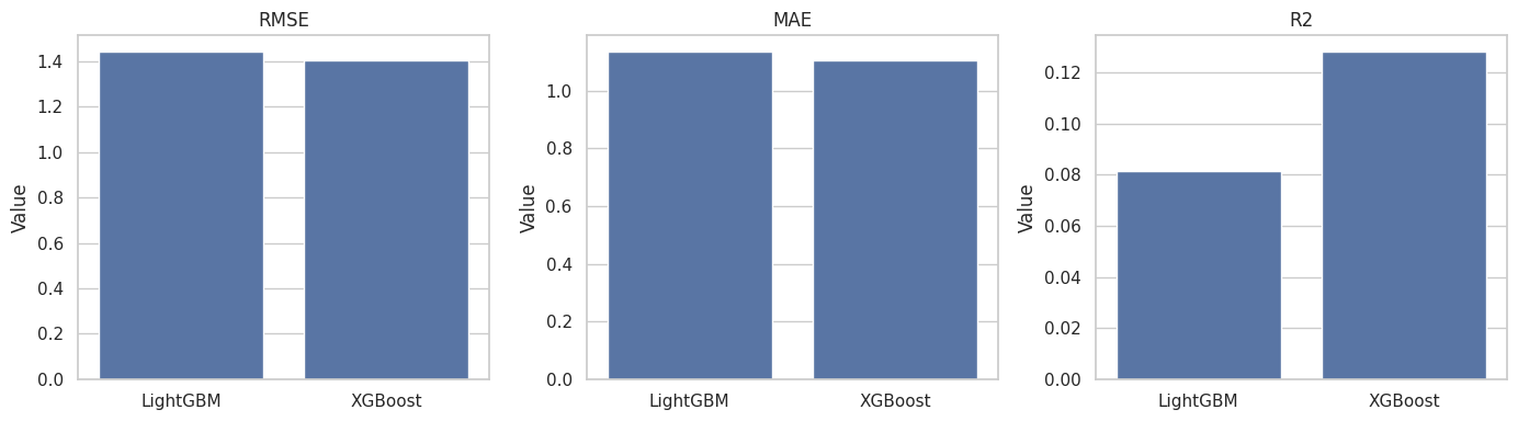
This plot compares model performance on the held-out test set. RMSE and MAE are in clicks per slate; R-squared shows how much outcome variation the model explains.

test_metrics_plot = model_metrics.query("split == 'test'").melt(
    id_vars="model",
    value_vars=["rmse", "mae", "r2"],
    var_name="metric",
    value_name="value",
)

fig, axes = plt.subplots(1, 3, figsize=(14, 4))
for ax, metric in zip(axes, ["rmse", "mae", "r2"]):
    sns.barplot(data=test_metrics_plot.query("metric == @metric"), x="model", y="value", ax=ax)
    ax.set_title(metric.upper())
    ax.set_xlabel("")
    ax.set_ylabel("Value")
plt.tight_layout()
fig.savefig(FIGURE_DIR / "20_advanced_model_metrics.png", dpi=160, bbox_inches="tight")
plt.show()

The model comparison is a reality check. If the models cannot predict slate outcomes at all, policy targeting will be unreliable. If they predict moderately well, they may still be useful for ranking slates by expected net effect.

8. Inspect Feature Importance

This cell extracts feature importance from LightGBM and XGBoost. The goal is to see whether the models are using sensible variables such as treatment assignment, focal position, slate composition, user history, and substitute counts.

importance_rows = []
for model_name, model in trained_models.items():
    importances = getattr(model, "feature_importances_", None)
    if importances is None:
        continue
    temp = pd.DataFrame(
        {
            "model": model_name,
            "feature": X.columns,
            "importance": importances,
        }
    )
    temp = temp.sort_values("importance", ascending=False)
    temp["rank"] = temp.groupby("model")["importance"].rank(method="first", ascending=False)
    importance_rows.append(temp)

feature_importance = pd.concat(importance_rows, ignore_index=True)
top_importance = feature_importance.query("rank <= 15").copy()

display(top_importance)
model feature importance rank
0 LightGBM slate_mean_log_popularity_z 539.0000 1.0000
1 LightGBM log_user_n_ratings 468.0000 2.0000
2 LightGBM slate_mean_sample_liked_rate 456.0000 3.0000
3 LightGBM log_focal_sample_rating_count 443.0000 4.0000
4 LightGBM liked_rate 377.0000 5.0000
5 LightGBM focal_sample_mean_rating 352.0000 6.0000
6 LightGBM mean_rating 336.0000 7.0000
7 LightGBM log_activity_span_days 321.0000 8.0000
8 LightGBM focal_sample_liked_rate 306.0000 9.0000
9 LightGBM slate_std_relevance 220.0000 10.0000
10 LightGBM slate_mean_relevance 209.0000 11.0000
11 LightGBM unique_primary_genres 131.0000 12.0000
12 LightGBM same_cluster_competitor_count 131.0000 13.0000
13 LightGBM focal_seed_position 122.0000 14.0000
14 LightGBM promotion_applied 80.0000 15.0000
51 XGBoost focal_observed_relevance 0.1913 1.0000
52 XGBoost slate_mean_relevance 0.1545 2.0000
53 XGBoost slate_high_relevance_rate 0.0357 3.0000
54 XGBoost liked_rate 0.0329 4.0000
55 XGBoost slate_mean_log_popularity_z 0.0262 5.0000
56 XGBoost focal_spillover_cluster_Animation 0.0240 6.0000
57 XGBoost same_cluster_competitor_count 0.0240 7.0000
58 XGBoost focal_spillover_cluster_Thriller 0.0239 8.0000
59 XGBoost slate_mean_sample_liked_rate 0.0231 9.0000
60 XGBoost promotion_applied 0.0223 10.0000
61 XGBoost focal_position_bucket_positions_7_9 0.0221 11.0000
62 XGBoost unique_primary_genres 0.0208 12.0000
63 XGBoost focal_sample_liked_rate 0.0206 13.0000
64 XGBoost mean_rating 0.0203 14.0000
65 XGBoost focal_log_item_popularity_z 0.0202 15.0000

Feature importance does not prove causality, but it helps audit the model. Sensible top features suggest the model is learning from pre-promotion slate structure rather than from artifacts. Treatment assignment and spillover-related features should matter if the model is capturing intervention effects.

9. Plot Top Feature Importance

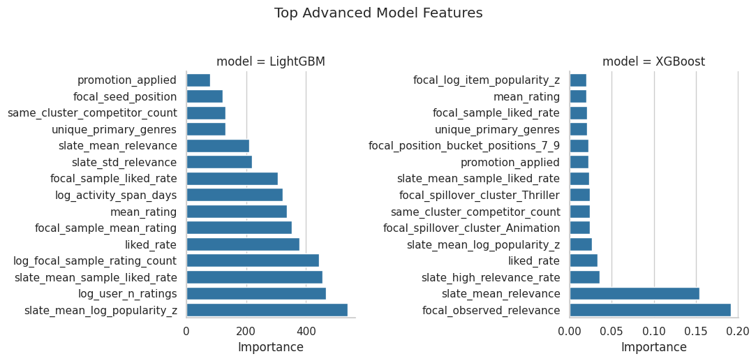
The table above is dense, so this plot shows the top model features in a compact format. Each model gets its own panel.

g = sns.FacetGrid(
    top_importance,
    col="model",
    sharex=False,
    sharey=False,
    height=5,
    aspect=1.1,
)

def importance_barplot(data, **kwargs):
    ordered = data.sort_values("importance", ascending=True)
    ax = plt.gca()
    sns.barplot(data=ordered, x="importance", y="feature", ax=ax, color="tab:blue")
    ax.set_xlabel("Importance")
    ax.set_ylabel("")

g.map_dataframe(importance_barplot)
g.fig.suptitle("Top Advanced Model Features", y=1.03)
plt.tight_layout()
g.fig.savefig(FIGURE_DIR / "21_advanced_feature_importance.png", dpi=160, bbox_inches="tight")
plt.show()

The feature plot is useful for communication: it shows which pre-promotion properties drive the model’s predictions. If focal position, relevance, and competitor counts appear, the model is aligned with the interference mechanism we care about.

10. Generate Counterfactual Predictions

This cell uses each trained outcome model to predict two potential outcomes for every slate:

  • predicted total clicks if the focal item is promoted,
  • predicted total clicks if the slate is left unchanged.

The difference between those predictions is a model-estimated conditional net effect. Because this is a simulation, we can compare that estimate with the reconstructed true expected promotion lift.

def counterfactual_feature_matrix(X_base, treatment_value):
    X_cf = X_base.copy()
    X_cf["promotion_applied"] = float(treatment_value)
    return X_cf

counterfactual_predictions = model_table[
    [
        "slate_id",
        "userId",
        "promotion_applied",
        "focal_seed_position",
        "focal_spillover_cluster",
        "total_simulated_clicks",
        "true_promote_lift",
    ]
].copy()

X_promote = counterfactual_feature_matrix(X, 1)
X_control = counterfactual_feature_matrix(X, 0)

counterfactual_summary_rows = []
for model_name, model in trained_models.items():
    pred_promote = model.predict(X_promote)
    pred_control = model.predict(X_control)
    pred_lift = pred_promote - pred_control
    counterfactual_predictions[f"pred_promote_clicks_{model_name}"] = pred_promote
    counterfactual_predictions[f"pred_control_clicks_{model_name}"] = pred_control
    counterfactual_predictions[f"pred_net_lift_{model_name}"] = pred_lift

    counterfactual_summary_rows.append(
        {
            "model": model_name,
            "mean_predicted_lift": pred_lift.mean(),
            "median_predicted_lift": np.median(pred_lift),
            "share_predicted_positive": (pred_lift > 0).mean(),
            "true_mean_lift": counterfactual_predictions["true_promote_lift"].mean(),
            "cate_rmse_vs_oracle": np.sqrt(mean_squared_error(counterfactual_predictions["true_promote_lift"], pred_lift)),
            "cate_mae_vs_oracle": mean_absolute_error(counterfactual_predictions["true_promote_lift"], pred_lift),
            "cate_correlation_vs_oracle": np.corrcoef(counterfactual_predictions["true_promote_lift"], pred_lift)[0, 1],
        }
    )

counterfactual_summary = pd.DataFrame(counterfactual_summary_rows).sort_values("cate_rmse_vs_oracle")
selected_cate_model = counterfactual_summary.iloc[0]["model"]
selected_cate_col = f"pred_net_lift_{selected_cate_model}"

display(counterfactual_summary)
print(f"Selected CATE model by oracle RMSE: {selected_cate_model}")
model mean_predicted_lift median_predicted_lift share_predicted_positive true_mean_lift cate_rmse_vs_oracle cate_mae_vs_oracle cate_correlation_vs_oracle
1 XGBoost -0.2388 -0.2361 0.0100 -0.3158 0.1610 0.1244 0.0189
0 LightGBM -0.2269 -0.2113 0.1267 -0.3158 0.2481 0.1967 0.0491
Selected CATE model by oracle RMSE: XGBoost

The oracle comparison is only possible because this is a simulation. A good advanced model should at least rank slates in the right direction, even if the exact predicted lift is noisy. The selected model will be used for policy targeting below.

11. Plot Predicted Net Lift Against Oracle Net Lift

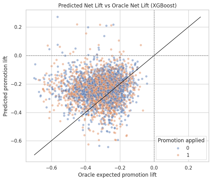
This scatter plot shows whether the selected model can identify slates with less harmful or more beneficial promotion effects. The diagonal line represents perfect prediction.

fig, ax = plt.subplots(figsize=(7, 6))
sns.scatterplot(
    data=counterfactual_predictions,
    x="true_promote_lift",
    y=selected_cate_col,
    hue="promotion_applied",
    alpha=0.45,
    s=28,
    ax=ax,
)
min_value = min(counterfactual_predictions["true_promote_lift"].min(), counterfactual_predictions[selected_cate_col].min())
max_value = max(counterfactual_predictions["true_promote_lift"].max(), counterfactual_predictions[selected_cate_col].max())
ax.plot([min_value, max_value], [min_value, max_value], color="black", linewidth=1)
ax.axhline(0, color="gray", linewidth=1, linestyle="--")
ax.axvline(0, color="gray", linewidth=1, linestyle="--")
ax.set_title(f"Predicted Net Lift vs Oracle Net Lift ({selected_cate_model})")
ax.set_xlabel("Oracle expected promotion lift")
ax.set_ylabel("Predicted promotion lift")
ax.legend(title="Promotion applied")
plt.tight_layout()
fig.savefig(FIGURE_DIR / "22_predicted_vs_oracle_net_lift.png", dpi=160, bbox_inches="tight")
plt.show()

The scatter plot should be read as a targeting diagnostic, not as a replacement for randomized estimation. The key question is whether higher predicted lift corresponds to higher oracle lift. If it does, the model can help prioritize safer promotions.

12. Cross-Fitted Model-Assisted AIPW Estimate

Even though assignment is randomized, we can use outcome models to build a model-assisted estimator. This cell fits separate LightGBM outcome models for treated and control slates using cross-fitting, then computes an augmented inverse probability weighted estimate.

The treatment probability is known: promotion was randomized with probability 0.5. Cross-fitting keeps each slate’s nuisance predictions out of sample.

def make_aipw_model(seed):
    return lgb.LGBMRegressor(
        n_estimators=250,
        learning_rate=0.04,
        num_leaves=15,
        min_child_samples=20,
        subsample=0.9,
        colsample_bytree=0.9,
        random_state=seed,
        verbose=-1,
    )

N_SPLITS = 5
PROPENSITY = 0.5
skf = StratifiedKFold(n_splits=N_SPLITS, shuffle=True, random_state=RANDOM_SEED)

m1_hat = np.zeros(len(model_table), dtype=float)
m0_hat = np.zeros(len(model_table), dtype=float)
fold_id = np.zeros(len(model_table), dtype=int)

for fold, (train_positions, holdout_positions) in enumerate(skf.split(X, treatment), start=1):
    X_train_fold = X.iloc[train_positions]
    y_train_fold = y.iloc[train_positions]
    t_train_fold = treatment.iloc[train_positions]

    model_treated = make_aipw_model(RANDOM_SEED + fold)
    model_control = make_aipw_model(RANDOM_SEED + 100 + fold)

    model_treated.fit(X_train_fold.loc[t_train_fold.eq(1)], y_train_fold.loc[t_train_fold.eq(1)])
    model_control.fit(X_train_fold.loc[t_train_fold.eq(0)], y_train_fold.loc[t_train_fold.eq(0)])

    m1_hat[holdout_positions] = model_treated.predict(counterfactual_feature_matrix(X.iloc[holdout_positions], 1))
    m0_hat[holdout_positions] = model_control.predict(counterfactual_feature_matrix(X.iloc[holdout_positions], 0))
    fold_id[holdout_positions] = fold

observed_y = y.to_numpy(dtype=float)
observed_t = treatment.to_numpy(dtype=float)

model_assisted_scores = (
    (m1_hat - m0_hat)
    + observed_t / PROPENSITY * (observed_y - m1_hat)
    - (1 - observed_t) / (1 - PROPENSITY) * (observed_y - m0_hat)
)

simple_difference = observed_y[observed_t == 1].mean() - observed_y[observed_t == 0].mean()
aipw_estimate = model_assisted_scores.mean()
aipw_se = model_assisted_scores.std(ddof=1) / np.sqrt(len(model_assisted_scores))

model_assisted_table = pd.DataFrame(
    [
        {
            "estimator": "Randomized difference in means",
            "estimate": simple_difference,
            "se": np.nan,
            "ci_95_lower": np.nan,
            "ci_95_upper": np.nan,
            "reference": "Observed total simulated clicks",
        },
        {
            "estimator": "Cross-fitted LightGBM AIPW",
            "estimate": aipw_estimate,
            "se": aipw_se,
            "ci_95_lower": aipw_estimate - 1.96 * aipw_se,
            "ci_95_upper": aipw_estimate + 1.96 * aipw_se,
            "reference": "Observed total simulated clicks",
        },
        {
            "estimator": "Oracle mean promotion lift",
            "estimate": model_table["true_promote_lift"].mean(),
            "se": model_table["true_promote_lift"].std(ddof=1) / np.sqrt(len(model_table)),
            "ci_95_lower": model_table["true_promote_lift"].mean() - 1.96 * model_table["true_promote_lift"].std(ddof=1) / np.sqrt(len(model_table)),
            "ci_95_upper": model_table["true_promote_lift"].mean() + 1.96 * model_table["true_promote_lift"].std(ddof=1) / np.sqrt(len(model_table)),
            "reference": "Known simulation lift",
        },
    ]
)

counterfactual_predictions["crossfit_m1_hat"] = m1_hat
counterfactual_predictions["crossfit_m0_hat"] = m0_hat
counterfactual_predictions["crossfit_cate_lgbm"] = m1_hat - m0_hat
counterfactual_predictions["aipw_score"] = model_assisted_scores
counterfactual_predictions["fold_id"] = fold_id

display(model_assisted_table)
estimator estimate se ci_95_lower ci_95_upper reference
0 Randomized difference in means -0.3078 NaN NaN NaN Observed total simulated clicks
1 Cross-fitted LightGBM AIPW -0.3036 0.0505 -0.4024 -0.2047 Observed total simulated clicks
2 Oracle mean promotion lift -0.3158 0.0019 -0.3195 -0.3120 Known simulation lift

The AIPW estimator is a robustness check. Because the design is randomized, the simple difference-in-means is already valid. The model-assisted estimate asks whether flexible outcome models produce a similar average answer while also generating useful conditional-effect predictions.

13. Model-Targeted Promotion Policies

This cell compares several targeting rules using the selected model’s predicted net lift. Since this is a simulation, the policies are evaluated using oracle expected promotion lift. In a real setting, this would require an online experiment or a valid off-policy evaluation design.

The table reports both value per selected slate and value per 1,000 eligible slates. The second metric accounts for how many slates the policy chooses to promote.

policy_scores = counterfactual_predictions.copy()
policy_scores["selected_model_predicted_lift"] = policy_scores[selected_cate_col]

predicted_lift = policy_scores["selected_model_predicted_lift"]
true_lift = policy_scores["true_promote_lift"]

policy_masks = {
    "Promote all eligible slates": np.ones(len(policy_scores), dtype=bool),
    "Promote top 50% by predicted net lift": predicted_lift >= predicted_lift.quantile(0.50),
    "Promote top 25% by predicted net lift": predicted_lift >= predicted_lift.quantile(0.75),
    "Promote only predicted-positive slates": predicted_lift > 0,
    "Oracle top 25% benchmark": true_lift >= true_lift.quantile(0.75),
}

policy_rows = []
for policy_name, mask in policy_masks.items():
    mask = np.asarray(mask, dtype=bool)
    selected_count = int(mask.sum())
    coverage = selected_count / len(policy_scores)
    if selected_count == 0:
        mean_predicted_selected = np.nan
        mean_true_selected = np.nan
        lift_per_1000_selected = np.nan
        lift_per_1000_eligible = 0.0
    else:
        mean_predicted_selected = predicted_lift[mask].mean()
        mean_true_selected = true_lift[mask].mean()
        lift_per_1000_selected = mean_true_selected * 1000
        lift_per_1000_eligible = true_lift[mask].sum() / len(policy_scores) * 1000
    policy_rows.append(
        {
            "policy": policy_name,
            "selected_slates": selected_count,
            "coverage": coverage,
            "mean_predicted_lift_selected": mean_predicted_selected,
            "mean_oracle_lift_selected": mean_true_selected,
            "oracle_lift_per_1000_selected_slates": lift_per_1000_selected,
            "oracle_lift_per_1000_eligible_slates": lift_per_1000_eligible,
        }
    )

policy_targeting = pd.DataFrame(policy_rows)

display(policy_targeting)
policy selected_slates coverage mean_predicted_lift_selected mean_oracle_lift_selected oracle_lift_per_1000_selected_slates oracle_lift_per_1000_eligible_slates
0 Promote all eligible slates 3000 1.0000 -0.2388 -0.3158 -315.7549 -315.7549
1 Promote top 50% by predicted net lift 1500 0.5000 -0.1648 -0.3091 -309.0693 -154.5346
2 Promote top 25% by predicted net lift 750 0.2500 -0.1213 -0.3065 -306.4754 -76.6188
3 Promote only predicted-positive slates 30 0.0100 0.0901 -0.3654 -365.3709 -3.6537
4 Oracle top 25% benchmark 750 0.2500 -0.2284 -0.1953 -195.3376 -48.8344

The targeting table shows whether the model can reduce harm by avoiding slates with strongly negative predicted net lift. The oracle benchmark is not deployable, but it shows the value available if targeting were perfect.

14. Plot Policy Targeting Results

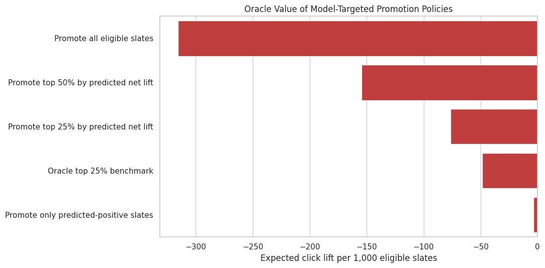
This plot compares the net oracle value of each promotion rule. The value is shown per 1,000 eligible slates, so policies that promote fewer slates are penalized for lower coverage.

policy_plot = policy_targeting.sort_values("oracle_lift_per_1000_eligible_slates", ascending=True).copy()

fig, ax = plt.subplots(figsize=(11, 5.5))
colors = ["tab:green" if value >= 0 else "tab:red" for value in policy_plot["oracle_lift_per_1000_eligible_slates"]]
sns.barplot(
    data=policy_plot,
    x="oracle_lift_per_1000_eligible_slates",
    y="policy",
    hue="policy",
    palette=dict(zip(policy_plot["policy"], colors)),
    legend=False,
    ax=ax,
)
ax.axvline(0, color="black", linewidth=1)
ax.set_title("Oracle Value of Model-Targeted Promotion Policies")
ax.set_xlabel("Expected click lift per 1,000 eligible slates")
ax.set_ylabel("")
plt.tight_layout()
fig.savefig(FIGURE_DIR / "23_policy_targeting_value.png", dpi=160, bbox_inches="tight")
plt.show()

The policy plot translates advanced modeling into a decision question. If targeted rules are less negative than promoting all slates, the model is useful even if it does not fully solve the problem. The safest policy may still be to avoid promotion unless predicted net value is positive.

15. Heterogeneity Diagnostics

This cell summarizes true and predicted net lift across interpretable segments: focal starting position, substitute count, displaced count, user activity, and focal cluster. The goal is to connect ML predictions back to product reasoning.

heterogeneity_frame = model_table[
    [
        "slate_id",
        "focal_seed_position",
        "focal_position_bucket",
        "focal_spillover_cluster",
        "same_cluster_competitor_count",
        "displaced_candidate_count",
        "n_ratings",
        "true_promote_lift",
    ]
].merge(
    policy_scores[["slate_id", "selected_model_predicted_lift"]],
    on="slate_id",
    how="left",
)

heterogeneity_frame["same_cluster_count_bucket"] = pd.cut(
    heterogeneity_frame["same_cluster_competitor_count"],
    bins=[-0.1, 0, 2, 5, 11],
    labels=["0", "1-2", "3-5", "6+"],
)
heterogeneity_frame["displaced_count_bucket"] = pd.cut(
    heterogeneity_frame["displaced_candidate_count"],
    bins=[-0.1, 4, 7, 11],
    labels=["4_or_fewer", "5-7", "8+"],
)
heterogeneity_frame["user_activity_bucket"] = pd.qcut(
    heterogeneity_frame["n_ratings"].rank(method="first"),
    q=4,
    labels=["lowest_activity", "low_mid_activity", "high_mid_activity", "highest_activity"],
)

def summarize_segment(frame, segment_type, segment_column, min_slates=30):
    summary = (
        frame.groupby(segment_column, observed=True)
        .agg(
            slates=("slate_id", "size"),
            mean_true_lift=("true_promote_lift", "mean"),
            mean_predicted_lift=("selected_model_predicted_lift", "mean"),
            share_positive_true_lift=("true_promote_lift", lambda s: (s > 0).mean()),
        )
        .reset_index()
        .rename(columns={segment_column: "segment"})
    )
    summary = summary.query("slates >= @min_slates").copy()
    summary["segment_type"] = segment_type
    return summary

heterogeneity_summaries = pd.concat(
    [
        summarize_segment(heterogeneity_frame, "focal_position_bucket", "focal_position_bucket"),
        summarize_segment(heterogeneity_frame, "same_cluster_count_bucket", "same_cluster_count_bucket"),
        summarize_segment(heterogeneity_frame, "displaced_count_bucket", "displaced_count_bucket"),
        summarize_segment(heterogeneity_frame, "user_activity_bucket", "user_activity_bucket"),
        summarize_segment(heterogeneity_frame, "focal_cluster", "focal_spillover_cluster", min_slates=60),
    ],
    ignore_index=True,
)
heterogeneity_summaries = heterogeneity_summaries.sort_values(["segment_type", "mean_true_lift"])

display(heterogeneity_summaries)
segment slates mean_true_lift mean_predicted_lift share_positive_true_lift segment_type
9 8+ 1472 -0.3478 -0.2735 0.0000 displaced_count_bucket
8 5-7 1162 -0.2961 -0.2121 0.0000 displaced_count_bucket
7 4_or_fewer 366 -0.2493 -0.1842 0.0000 displaced_count_bucket
14 Action 799 -0.3625 -0.2154 0.0000 focal_cluster
17 Comedy 658 -0.3258 -0.2348 0.0000 focal_cluster
19 Drama 636 -0.3221 -0.2426 0.0000 focal_cluster
15 Adventure 318 -0.2784 -0.2439 0.0000 focal_cluster
18 Crime 253 -0.2725 -0.2623 0.0000 focal_cluster
16 Animation 70 -0.2496 -0.2290 0.0000 focal_cluster
20 Horror 65 -0.2378 -0.2969 0.0000 focal_cluster
2 positions_10_12 1086 -0.3535 -0.2775 0.0000 focal_position_bucket
1 positions_7_9 1168 -0.3119 -0.2362 0.0000 focal_position_bucket
0 positions_5_6 746 -0.2668 -0.1867 0.0000 focal_position_bucket
6 6+ 427 -0.4598 -0.2174 0.0000 same_cluster_count_bucket
5 3-5 1006 -0.3471 -0.2264 0.0000 same_cluster_count_bucket
4 1-2 1023 -0.2729 -0.2280 0.0000 same_cluster_count_bucket
3 0 544 -0.2253 -0.2990 0.0000 same_cluster_count_bucket
10 lowest_activity 750 -0.3386 -0.2512 0.0000 user_activity_bucket
11 low_mid_activity 750 -0.3327 -0.2277 0.0000 user_activity_bucket
12 high_mid_activity 750 -0.3145 -0.2338 0.0000 user_activity_bucket
13 highest_activity 750 -0.2772 -0.2426 0.0000 user_activity_bucket

The heterogeneity table makes the targeting story interpretable. Segments with less negative or positive true lift are safer promotion candidates. Segments with many substitutes or large displacement exposure are more likely to show negative net effects.

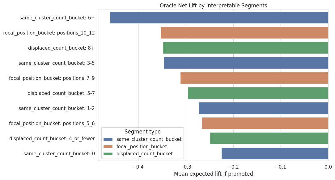
16. Plot Interpretable Heterogeneity

This plot focuses on the most actionable segment types: focal starting position and same-cluster competitor count. These are directly tied to the mechanism of item competition.

heterogeneity_plot = heterogeneity_summaries.query(
    "segment_type in ['focal_position_bucket', 'same_cluster_count_bucket', 'displaced_count_bucket']"
).copy()
heterogeneity_plot["segment_label"] = heterogeneity_plot["segment_type"] + ": " + heterogeneity_plot["segment"].astype(str)

fig, ax = plt.subplots(figsize=(11, 6))
sns.barplot(
    data=heterogeneity_plot.sort_values("mean_true_lift"),
    x="mean_true_lift",
    y="segment_label",
    hue="segment_type",
    dodge=False,
    ax=ax,
)
ax.axvline(0, color="black", linewidth=1)
ax.set_title("Oracle Net Lift by Interpretable Segments")
ax.set_xlabel("Mean expected lift if promoted")
ax.set_ylabel("")
ax.legend(title="Segment type")
plt.tight_layout()
fig.savefig(FIGURE_DIR / "24_advanced_heterogeneity_segments.png", dpi=160, bbox_inches="tight")
plt.show()

The segment plot connects advanced modeling back to recommendation design. If promotions are most harmful in slates with many displaced or same-cluster competitors, then safer policies should account for local slate competition before promoting an item.

17. Advanced Modeling Takeaways Table

This cell creates a compact summary table for the final report. It records what the advanced models added beyond the transparent randomized estimators.

best_metrics = model_metrics.query("split == 'test' and model == @best_model_name").iloc[0]
best_counterfactual = counterfactual_summary.query("model == @selected_cate_model").iloc[0]
best_policy = policy_targeting.sort_values("oracle_lift_per_1000_eligible_slates", ascending=False).iloc[0]

advanced_takeaways = pd.DataFrame(
    [
        {
            "area": "Outcome modeling",
            "finding": f"{best_model_name} had the best held-out RMSE at {best_metrics['rmse']:.3f} clicks per slate.",
            "why_it_matters": "Flexible models can summarize how slate composition and treatment assignment relate to total outcomes.",
        },
        {
            "area": "Conditional effects",
            "finding": f"{selected_cate_model} had CATE RMSE {best_counterfactual['cate_rmse_vs_oracle']:.3f} versus the oracle simulation lift.",
            "why_it_matters": "The model can be used to rank slates by predicted net harm or benefit, with simulation validation.",
        },
        {
            "area": "Model-assisted estimation",
            "finding": f"Cross-fitted AIPW estimated {aipw_estimate:.3f} total clicks per slate, compared with {simple_difference:.3f} from the randomized difference-in-means.",
            "why_it_matters": "Model-assisted estimates should agree with the randomized baseline before being used for targeting.",
        },
        {
            "area": "Policy targeting",
            "finding": f"The best evaluated policy was '{best_policy['policy']}' with {best_policy['oracle_lift_per_1000_eligible_slates']:.1f} oracle lift per 1,000 eligible slates.",
            "why_it_matters": "Targeting can reduce displacement harm compared with promoting every eligible slate.",
        },
    ]
)

display(advanced_takeaways)
area finding why_it_matters
0 Outcome modeling XGBoost had the best held-out RMSE at 1.405 cl... Flexible models can summarize how slate compos...
1 Conditional effects XGBoost had CATE RMSE 0.161 versus the oracle ... The model can be used to rank slates by predic...
2 Model-assisted estimation Cross-fitted AIPW estimated -0.304 total click... Model-assisted estimates should agree with the...
3 Policy targeting The best evaluated policy was 'Promote only pr... Targeting can reduce displacement harm compare...

This table is designed for the final report. It keeps the advanced work concrete: model performance, conditional-effect validation, model-assisted estimation, and policy targeting.

18. Save Advanced Modeling Outputs

This cell saves all advanced modeling artifacts. The final report notebook can load these directly rather than recomputing models.

MODEL_METRICS_OUTPUT = PROCESSED_DIR / "movielens_interference_advanced_model_metrics.csv"
FEATURE_IMPORTANCE_OUTPUT = PROCESSED_DIR / "movielens_interference_advanced_feature_importance.csv"
COUNTERFACTUAL_OUTPUT = PROCESSED_DIR / "movielens_interference_advanced_counterfactual_predictions.parquet"
COUNTERFACTUAL_SUMMARY_OUTPUT = PROCESSED_DIR / "movielens_interference_advanced_counterfactual_summary.csv"
AIPW_OUTPUT = PROCESSED_DIR / "movielens_interference_advanced_aipw_estimates.csv"
POLICY_OUTPUT = PROCESSED_DIR / "movielens_interference_advanced_policy_targeting.csv"
HETEROGENEITY_OUTPUT = PROCESSED_DIR / "movielens_interference_advanced_heterogeneity.csv"
TAKEAWAYS_OUTPUT = PROCESSED_DIR / "movielens_interference_advanced_takeaways.csv"

model_metrics.to_csv(MODEL_METRICS_OUTPUT, index=False)
feature_importance.to_csv(FEATURE_IMPORTANCE_OUTPUT, index=False)
counterfactual_predictions.to_parquet(COUNTERFACTUAL_OUTPUT, index=False)
counterfactual_summary.to_csv(COUNTERFACTUAL_SUMMARY_OUTPUT, index=False)
model_assisted_table.to_csv(AIPW_OUTPUT, index=False)
policy_targeting.to_csv(POLICY_OUTPUT, index=False)
heterogeneity_summaries.to_csv(HETEROGENEITY_OUTPUT, index=False)
advanced_takeaways.to_csv(TAKEAWAYS_OUTPUT, index=False)

saved_outputs = pd.DataFrame(
    {
        "artifact": [
            "model_metrics",
            "feature_importance",
            "counterfactual_predictions",
            "counterfactual_summary",
            "aipw_estimates",
            "policy_targeting",
            "heterogeneity",
            "advanced_takeaways",
        ],
        "path": [
            str(MODEL_METRICS_OUTPUT),
            str(FEATURE_IMPORTANCE_OUTPUT),
            str(COUNTERFACTUAL_OUTPUT),
            str(COUNTERFACTUAL_SUMMARY_OUTPUT),
            str(AIPW_OUTPUT),
            str(POLICY_OUTPUT),
            str(HETEROGENEITY_OUTPUT),
            str(TAKEAWAYS_OUTPUT),
        ],
    }
)

display(saved_outputs)
artifact path
0 model_metrics /home/apex/Documents/ranking_sys/data/processe...
1 feature_importance /home/apex/Documents/ranking_sys/data/processe...
2 counterfactual_predictions /home/apex/Documents/ranking_sys/data/processe...
3 counterfactual_summary /home/apex/Documents/ranking_sys/data/processe...
4 aipw_estimates /home/apex/Documents/ranking_sys/data/processe...
5 policy_targeting /home/apex/Documents/ranking_sys/data/processe...
6 heterogeneity /home/apex/Documents/ranking_sys/data/processe...
7 advanced_takeaways /home/apex/Documents/ranking_sys/data/processe...

The saved files complete the advanced-modeling handoff. The key artifacts are the counterfactual predictions, AIPW estimate table, policy targeting table, and advanced takeaways.

19. Notebook Takeaways

This notebook added advanced modeling without changing the causal foundation:

  • LightGBM and XGBoost were trained to predict total slate outcomes from pre-promotion features and treatment assignment.
  • Counterfactual predictions estimated conditional net promotion effects for each slate.
  • A cross-fitted model-assisted AIPW estimate was compared with the simple randomized estimator.
  • Targeted promotion rules were evaluated against the oracle simulation lift.
  • Heterogeneity summaries showed where promotion is most likely to be safer or more harmful.

The final notebook should now package the full workflow: dataset setup, exposure mapping, randomized estimators, direct/indirect/total decomposition, advanced models, assumptions, limitations, figures, tables, and portfolio-ready writing.