Cluster-Randomized Estimators for Direct and Spillover Effects

This notebook is the first causal estimation notebook in the interference and spillover workflow.

The previous notebook created a randomized promotion simulation from MovieLens seed slates. In each slate, one lower-ranked focal movie was selected, and the slate was randomized to either promote that focal movie or leave the slate unchanged. That gives us a clean assignment mechanism:

The goal here is to estimate what changed when promotion was randomized:

  1. Direct focal effect: what happens to the promoted movie?
  2. Same-cluster spillover effect: what happens to substitute movies in the same slate?
  3. Displaced-item spillover effect: what happens to items that are pushed down by promotion?
  4. Total slate effect: what happens to total slate engagement after combining gains and losses?

Because treatment is assigned at the slate level, uncertainty should respect slate clustering. The notebook therefore compares naive standard errors with slate-clustered standard errors and also uses a cluster bootstrap as a non-parametric check.

1. Environment and Paths

This cell imports the estimation, plotting, and table tools used in the notebook. It also finds the repository root by searching upward for the exposure mapping file, which keeps the notebook robust across Jupyter and command-line execution.

from pathlib import Path

import matplotlib.pyplot as plt
import numpy as np
import pandas as pd
import seaborn as sns
import statsmodels.api as sm
from IPython.display import display

sns.set_theme(style="whitegrid", context="notebook")
pd.set_option("display.max_columns", 120)
pd.set_option("display.max_rows", 100)
pd.set_option("display.float_format", lambda value: f"{value:,.4f}")

candidate_roots = [Path.cwd(), *Path.cwd().parents]
PROJECT_DIR = next(
    root for root in candidate_roots
    if (root / "data" / "processed" / "movielens_interference_exposure_mapping.parquet").exists()
)

PROCESSED_DIR = PROJECT_DIR / "data" / "processed"
NOTEBOOK_DIR = PROJECT_DIR / "notebooks" / "interference_spillover_effects"
WRITEUP_DIR = NOTEBOOK_DIR / "writeup"
FIGURE_DIR = WRITEUP_DIR / "figures"
TABLE_DIR = WRITEUP_DIR / "tables"
FIGURE_DIR.mkdir(parents=True, exist_ok=True)
TABLE_DIR.mkdir(parents=True, exist_ok=True)

EXPOSURE_PATH = PROCESSED_DIR / "movielens_interference_exposure_mapping.parquet"
SLATE_OUTCOME_PATH = PROCESSED_DIR / "movielens_interference_slate_outcomes.parquet"
ASSIGNMENT_PATH = PROCESSED_DIR / "movielens_interference_assignment_table.parquet"

EXPOSURE_PATH.exists(), SLATE_OUTCOME_PATH.exists(), ASSIGNMENT_PATH.exists()
(True, True, True)

All three checks should be True. The notebook depends on the item-row exposure table, the slate-level outcome table, and the focal assignment table produced in the previous notebook.

2. Load the Randomized Exposure Data

This cell loads the analysis-ready data. The item-row table is used for direct and spillover contrasts, while the slate-level table is used for total-effect estimates. The assignment table is useful for checking that the randomized design is still intact.

exposure = pd.read_parquet(EXPOSURE_PATH)
slate_outcomes = pd.read_parquet(SLATE_OUTCOME_PATH)
assignment = pd.read_parquet(ASSIGNMENT_PATH)

load_summary = pd.DataFrame(
    {
        "table": ["item_row_exposure", "slate_outcomes", "assignment"],
        "rows": [len(exposure), len(slate_outcomes), len(assignment)],
        "unique_slates": [
            exposure["slate_id"].nunique(),
            slate_outcomes["slate_id"].nunique(),
            assignment["slate_id"].nunique(),
        ],
        "unique_users": [
            exposure["userId"].nunique(),
            slate_outcomes["userId"].nunique(),
            assignment["userId"].nunique(),
        ],
    }
)

display(load_summary)
display(exposure.head())
table rows unique_slates unique_users
0 item_row_exposure 36000 3000 3000
1 slate_outcomes 3000 3000 3000
2 assignment 3000 3000 3000
slate_id userId movieId title genres primary_genre spillover_cluster slate_position_seed observed_relevance high_relevance rating_datetime rating_year sample_rating_count sample_mean_rating sample_liked_rate popularity_bucket n_ratings mean_rating liked_rate active_years unique_primary_genres activity_span_days focal_movieId focal_title focal_spillover_cluster focal_seed_position promotion_probability promotion_applied assignment_arm is_focal_item direct_treatment same_slate_spillover same_cluster_spillover displaced_by_promotion final_position baseline_visibility final_visibility visibility_gain position_change exposure_group log_item_popularity log_item_popularity_z p_no_promotion p_observed known_probability_lift simulated_click simulated_engagement_score
0 user_50_seed 50 4027 O Brother, Where Art Thou? (2000) Adventure|Comedy|Crime Adventure Adventure 1 5.0000 1 2009-12-31 06:58:12 2009 581 3.8563 0.6644 very_high 118 4.2203 0.8051 1 11 1 1288 This Is Spinal Tap (1984) Comedy 6 0.5000 1 promote_focal_item 0 0 1 0 1 2 1.0000 0.6309 -0.3691 1 other_slate_spillover 6.3665 0.6853 0.4356 0.2966 -0.1390 1 1.7500
1 user_50_seed 50 1196 Star Wars: Episode V - The Empire Strikes Back... Action|Adventure|Sci-Fi Action Action 2 5.0000 1 2009-12-29 09:12:16 2009 1446 4.0992 0.7510 very_high 118 4.2203 0.8051 1 11 1 1288 This Is Spinal Tap (1984) Comedy 6 0.5000 1 promote_focal_item 0 0 1 0 1 3 0.6309 0.5000 -0.1309 1 other_slate_spillover 7.2772 1.3316 0.3550 0.2834 -0.0716 0 0.0000
2 user_50_seed 50 47 Seven (a.k.a. Se7en) (1995) Mystery|Thriller Mystery Mystery 3 5.0000 1 2009-12-29 09:11:39 2009 1247 4.0545 0.7257 very_high 118 4.2203 0.8051 1 11 1 1288 This Is Spinal Tap (1984) Comedy 6 0.5000 1 promote_focal_item 0 0 1 0 1 4 0.5000 0.4307 -0.0693 1 other_slate_spillover 7.1293 1.2266 0.3176 0.2642 -0.0535 0 0.0000
3 user_50_seed 50 52435 How the Grinch Stole Christmas! (1966) Animation|Comedy|Fantasy|Musical Animation Animation 4 5.0000 1 2009-12-29 09:10:49 2009 43 3.9070 0.6512 very_high 118 4.2203 0.8051 1 11 1 1288 This Is Spinal Tap (1984) Comedy 6 0.5000 1 promote_focal_item 0 0 1 0 1 5 0.4307 0.3869 -0.0438 1 other_slate_spillover 3.7842 -1.1469 0.2497 0.2090 -0.0406 0 0.0000
4 user_50_seed 50 1214 Alien (1979) Horror|Sci-Fi Horror Horror 5 5.0000 1 2009-12-29 09:09:28 2009 832 4.1088 0.7404 very_high 118 4.2203 0.8051 1 11 1 1288 This Is Spinal Tap (1984) Comedy 6 0.5000 1 promote_focal_item 0 0 1 0 1 6 0.3869 0.3562 -0.0306 1 other_slate_spillover 6.7250 0.9397 0.2850 0.2432 -0.0418 1 1.7500

The row counts should line up with the previous notebook: 36,000 item rows and 3,000 slates. This confirms that every estimator in this notebook is working from the same randomized experiment simulation.

3. Recheck the Randomized Assignment

Before estimating effects, we recheck the promotion rate and the number of treated/control slates. This is a quick guard against accidental filtering that could break the randomized design.

assignment_check = (
    assignment.groupby("assignment_arm")
    .agg(
        slates=("slate_id", "size"),
        promotion_rate=("promotion_applied", "mean"),
        mean_focal_seed_position=("focal_seed_position", "mean"),
        mean_focal_relevance=("focal_observed_relevance", "mean"),
        high_relevance_rate=("focal_high_relevance", "mean"),
    )
    .reset_index()
)
assignment_check["slate_share"] = assignment_check["slates"] / assignment_check["slates"].sum()

display(assignment_check)
assignment_arm slates promotion_rate mean_focal_seed_position mean_focal_relevance high_relevance_rate slate_share
0 leave_slate_unchanged 1495 0.0000 8.4468 4.4893 0.9391 0.4983
1 promote_focal_item 1505 1.0000 8.4930 4.4897 0.9522 0.5017

The promoted and control arms should be nearly equal in size. Focal seed position and focal relevance should also be close across arms because promotion was randomized after focal item selection.

4. Define Estimation Helpers

This cell defines reusable functions for difference-in-means estimation. The basic estimator is a regression of an outcome on the randomized treatment indicator. For row-level item outcomes, standard errors are clustered by slate because all item rows in the same slate share the same randomized assignment and attention budget.

The helper returns both naive and cluster-robust uncertainty so we can see how much clustering matters.

def difference_in_means(
    data,
    outcome,
    treatment="promotion_applied",
    cluster_col="slate_id",
    contrast_name=None,
    outcome_label=None,
):
    # Estimate treated-control mean difference with naive and clustered uncertainty.
    columns = [outcome, treatment]
    if cluster_col is not None:
        columns.append(cluster_col)
    work = data[columns].dropna().copy()
    work[treatment] = work[treatment].astype(float)
    work[outcome] = work[outcome].astype(float)

    treated = work.loc[work[treatment] == 1, outcome]
    control = work.loc[work[treatment] == 0, outcome]
    if treated.empty or control.empty:
        raise ValueError(f"Both treatment arms are required for {contrast_name} / {outcome}.")

    x = sm.add_constant(work[treatment], has_constant="add")
    y = work[outcome]
    naive_fit = sm.OLS(y, x).fit()
    coef = float(naive_fit.params[treatment])
    naive_se = float(naive_fit.bse[treatment])

    if cluster_col is not None:
        cluster_fit = sm.OLS(y, x).fit(
            cov_type="cluster",
            cov_kwds={"groups": work[cluster_col]},
        )
        cluster_se = float(cluster_fit.bse[treatment])
        p_value = float(cluster_fit.pvalues[treatment])
        clusters = work[cluster_col].nunique()
    else:
        cluster_se = naive_se
        p_value = float(naive_fit.pvalues[treatment])
        clusters = np.nan

    return {
        "contrast": contrast_name or outcome,
        "outcome": outcome_label or outcome,
        "estimate": coef,
        "naive_se": naive_se,
        "cluster_se": cluster_se,
        "ci_95_lower": coef - 1.96 * cluster_se,
        "ci_95_upper": coef + 1.96 * cluster_se,
        "p_value_cluster": p_value,
        "treated_mean": treated.mean(),
        "control_mean": control.mean(),
        "treated_n": len(treated),
        "control_n": len(control),
        "clusters": clusters,
    }


def cluster_bootstrap_difference(
    data,
    outcome,
    treatment="promotion_applied",
    cluster_col="slate_id",
    n_bootstrap=500,
    seed=20260428,
):
    # Resample whole slates, then recompute the treated-control mean difference.
    work = data[[outcome, treatment, cluster_col]].dropna().reset_index(drop=True).copy()
    work[treatment] = work[treatment].astype(int)
    work[outcome] = work[outcome].astype(float)

    clusters = work[cluster_col].drop_duplicates().to_numpy()
    group_positions = work.groupby(cluster_col).indices
    rng = np.random.default_rng(seed)
    estimates = []

    for _ in range(n_bootstrap):
        sampled_clusters = rng.choice(clusters, size=len(clusters), replace=True)
        sampled_positions = np.concatenate([group_positions[cluster] for cluster in sampled_clusters])
        sample = work.iloc[sampled_positions]
        treated = sample.loc[sample[treatment] == 1, outcome]
        control = sample.loc[sample[treatment] == 0, outcome]
        if treated.empty or control.empty:
            estimates.append(np.nan)
        else:
            estimates.append(treated.mean() - control.mean())

    return np.asarray(estimates, dtype=float)

These helpers keep the estimation cells readable. The estimates are still simple difference-in-means estimators, but the implementation respects the randomized unit and returns enough diagnostic information to explain the uncertainty.

5. Define the Main Causal Contrasts

This cell creates the datasets for each contrast.

  • Direct focal effect uses only focal-item rows and compares promoted focal items with control focal items.
  • Same-cluster spillover effect uses non-focal movies in the same cluster as the focal movie. In promoted slates, these are substitute competitors exposed to spillover; in control slates, they are comparable substitute competitors without promotion.
  • Displaced-item spillover effect uses non-focal items that start above the focal item and therefore would be pushed down if the focal item is promoted.
  • All non-focal spillover effect looks at every non-focal item in promoted versus control slates.
  • Total slate effect uses one row per slate and measures the net outcome across all slate items.
focal_rows = exposure.query("is_focal_item == 1").copy()

same_cluster_candidates = exposure.query(
    "is_focal_item == 0 and spillover_cluster == focal_spillover_cluster"
).copy()

would_be_displaced_candidates = exposure.query(
    "is_focal_item == 0 and slate_position_seed < focal_seed_position"
).copy()

non_focal_rows = exposure.query("is_focal_item == 0").copy()

contrast_datasets = {
    "Direct focal item": focal_rows,
    "Same-cluster competitor spillover": same_cluster_candidates,
    "Displaced-item spillover": would_be_displaced_candidates,
    "All non-focal slate spillover": non_focal_rows,
    "Total slate": slate_outcomes.copy(),
}

contrast_summary = []
for name, df in contrast_datasets.items():
    contrast_summary.append(
        {
            "contrast": name,
            "rows": len(df),
            "slates": df["slate_id"].nunique(),
            "treated_rows_or_slates": int(df["promotion_applied"].sum()),
            "control_rows_or_slates": int((1 - df["promotion_applied"]).sum()),
            "treatment_rate": df["promotion_applied"].mean(),
        }
    )
contrast_summary = pd.DataFrame(contrast_summary)

display(contrast_summary)
contrast rows slates treated_rows_or_slates control_rows_or_slates treatment_rate
0 Direct focal item 3000 3000 1505 1495 0.5017
1 Same-cluster competitor spillover 8448 2456 4309 4139 0.5101
2 Displaced-item spillover 22410 3000 11277 11133 0.5032
3 All non-focal slate spillover 33000 3000 16555 16445 0.5017
4 Total slate 3000 3000 1505 1495 0.5017

The contrast summary shows how much support each estimator has. The same-cluster and displaced-item contrasts have many rows, but the randomized clusters are still slates. That is why the later standard errors are clustered by slate_id rather than treating every row as independent.

6. Estimate Direct, Spillover, and Total Effects

This cell estimates each contrast for three outcome views:

  • Observed simulated outcome: the noisy simulated click outcome generated in the previous notebook.
  • Expected probability outcome: the simulation’s expected click probability, which removes Bernoulli noise.
  • Known induced lift: the known probability change introduced by the promotion and spillover simulation.

The noisy outcome is what a real logged experiment would look like. The expected and known-lift outcomes are validation views available because this is a simulation.

estimation_jobs = [
    {
        "contrast": "Direct focal item",
        "data": focal_rows,
        "outcomes": [
            ("simulated_click", "Observed simulated click"),
            ("p_observed", "Expected click probability"),
            ("known_probability_lift", "Known induced probability lift"),
        ],
    },
    {
        "contrast": "Same-cluster competitor spillover",
        "data": same_cluster_candidates,
        "outcomes": [
            ("simulated_click", "Observed simulated click"),
            ("p_observed", "Expected click probability"),
            ("known_probability_lift", "Known induced probability lift"),
        ],
    },
    {
        "contrast": "Displaced-item spillover",
        "data": would_be_displaced_candidates,
        "outcomes": [
            ("simulated_click", "Observed simulated click"),
            ("p_observed", "Expected click probability"),
            ("known_probability_lift", "Known induced probability lift"),
        ],
    },
    {
        "contrast": "All non-focal slate spillover",
        "data": non_focal_rows,
        "outcomes": [
            ("simulated_click", "Observed simulated click"),
            ("p_observed", "Expected click probability"),
            ("known_probability_lift", "Known induced probability lift"),
        ],
    },
    {
        "contrast": "Total slate",
        "data": slate_outcomes,
        "outcomes": [
            ("total_simulated_clicks", "Observed total simulated clicks"),
            ("total_expected_clicks", "Expected total clicks"),
            ("total_known_probability_lift", "Known total probability lift"),
        ],
    },
]

estimate_rows = []
for job in estimation_jobs:
    for outcome, outcome_label in job["outcomes"]:
        estimate_rows.append(
            difference_in_means(
                job["data"],
                outcome=outcome,
                treatment="promotion_applied",
                cluster_col="slate_id",
                contrast_name=job["contrast"],
                outcome_label=outcome_label,
            )
        )

estimate_table = pd.DataFrame(estimate_rows)
estimate_table["cluster_to_naive_se_ratio"] = estimate_table["cluster_se"] / estimate_table["naive_se"]

display(estimate_table)
contrast outcome estimate naive_se cluster_se ci_95_lower ci_95_upper p_value_cluster treated_mean control_mean treated_n control_n clusters cluster_to_naive_se_ratio
0 Direct focal item Observed simulated click 0.1716 0.0157 0.0157 0.1409 0.2023 0.0000 0.3435 0.1719 1505 1495 3000 0.9992
1 Direct focal item Expected click probability 0.1777 0.0031 0.0031 0.1715 0.1838 0.0000 0.3556 0.1779 1505 1495 3000 0.9986
2 Direct focal item Known induced probability lift 0.1794 0.0010 0.0010 0.1774 0.1814 0.0000 0.1794 0.0000 1505 1495 3000 0.9967
3 Same-cluster competitor spillover Observed simulated click -0.0577 0.0083 0.0084 -0.0743 -0.0412 0.0000 0.1522 0.2100 4309 4139 2456 1.0107
4 Same-cluster competitor spillover Expected click probability -0.0695 0.0015 0.0024 -0.0742 -0.0648 0.0000 0.1466 0.2161 4309 4139 2456 1.5617
5 Same-cluster competitor spillover Known induced probability lift -0.0686 0.0006 0.0006 -0.0699 -0.0674 0.0000 -0.0686 0.0000 4309 4139 2456 1.0315
6 Displaced-item spillover Observed simulated click -0.0568 0.0054 0.0057 -0.0679 -0.0457 0.0000 0.1818 0.2386 11277 11133 3000 1.0419
7 Displaced-item spillover Expected click probability -0.0574 0.0010 0.0019 -0.0612 -0.0536 0.0000 0.1807 0.2380 11277 11133 3000 1.9139
8 Displaced-item spillover Known induced probability lift -0.0580 0.0004 0.0004 -0.0588 -0.0573 0.0000 -0.0580 0.0000 11277 11133 3000 1.0182
9 All non-focal slate spillover Observed simulated click -0.0436 0.0043 0.0046 -0.0526 -0.0346 0.0000 0.1705 0.2141 16555 16445 3000 1.0635
10 All non-focal slate spillover Expected click probability -0.0450 0.0008 0.0018 -0.0485 -0.0414 0.0000 0.1701 0.2151 16555 16445 3000 2.1522
11 All non-focal slate spillover Known induced probability lift -0.0452 0.0003 0.0003 -0.0458 -0.0447 0.0000 -0.0452 0.0000 16555 16445 3000 0.9693
12 Total slate Observed total simulated clicks -0.3078 0.0538 0.0538 -0.4132 -0.2024 0.0000 2.2193 2.5271 1505 1495 3000 1.0001
13 Total slate Expected total clicks -0.3168 0.0225 0.0226 -0.3610 -0.2726 0.0000 2.2269 2.5438 1505 1495 3000 1.0004
14 Total slate Known total probability lift -0.3180 0.0026 0.0026 -0.3232 -0.3129 0.0000 -0.3180 0.0000 1505 1495 3000 0.9967

The signs should tell the main story: promoted focal items gain, substitute or displaced competitors lose, and the total slate effect can be smaller than the direct gain because attention is reallocated. The cluster-to-naive standard error ratio shows whether row-level uncertainty would have been too optimistic.

7. Focus on the Noisy Observed Outcomes

The previous table includes validation outcomes that we only have because the data are simulated. This cell extracts the noisy observed-outcome estimates, which are the closest analogue to what we would report from a real randomized experiment.

observed_outcome_labels = [
    "Observed simulated click",
    "Observed total simulated clicks",
]

contrast_order = {
    "Direct focal item": 0,
    "Same-cluster competitor spillover": 1,
    "Displaced-item spillover": 2,
    "All non-focal slate spillover": 3,
    "Total slate": 4,
}

observed_estimates = estimate_table.loc[
    estimate_table["outcome"].isin(observed_outcome_labels)
].copy()
observed_estimates["contrast_order"] = observed_estimates["contrast"].map(contrast_order)
observed_estimates = observed_estimates.sort_values("contrast_order")

observed_estimates_display = observed_estimates[
    [
        "contrast",
        "outcome",
        "estimate",
        "cluster_se",
        "ci_95_lower",
        "ci_95_upper",
        "treated_mean",
        "control_mean",
        "treated_n",
        "control_n",
        "clusters",
    ]
]

display(observed_estimates_display)
contrast outcome estimate cluster_se ci_95_lower ci_95_upper treated_mean control_mean treated_n control_n clusters
0 Direct focal item Observed simulated click 0.1716 0.0157 0.1409 0.2023 0.3435 0.1719 1505 1495 3000
3 Same-cluster competitor spillover Observed simulated click -0.0577 0.0084 -0.0743 -0.0412 0.1522 0.2100 4309 4139 2456
6 Displaced-item spillover Observed simulated click -0.0568 0.0057 -0.0679 -0.0457 0.1818 0.2386 11277 11133 3000
9 All non-focal slate spillover Observed simulated click -0.0436 0.0046 -0.0526 -0.0346 0.1705 0.2141 16555 16445 3000
12 Total slate Observed total simulated clicks -0.3078 0.0538 -0.4132 -0.2024 2.2193 2.5271 1505 1495 3000

This table is the clean experiment-style result. The direct effect is the promoted focal item’s gain. The spillover rows measure competitor losses. The total slate row tells us whether the promotion helped the whole slate after accounting for displacement.

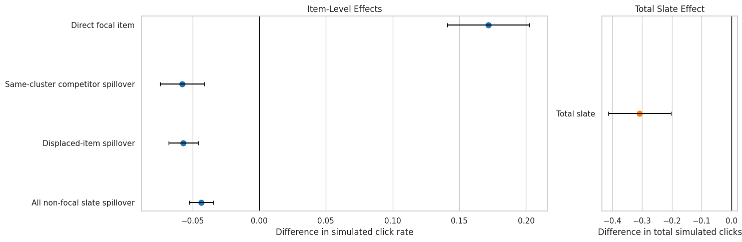
8. Plot Observed Estimates with Cluster-Robust Intervals

This plot shows the main observed estimates with 95 percent intervals using slate-clustered standard errors. Item-level and slate-level outcomes use different units, so the plot is split into item-row effects and total-slate effects.

item_observed = observed_estimates.query("contrast != 'Total slate'").copy()
slate_observed = observed_estimates.query("contrast == 'Total slate'").copy()

fig, axes = plt.subplots(1, 2, figsize=(15, 5), gridspec_kw={"width_ratios": [3, 1]})

sns.pointplot(
    data=item_observed,
    x="estimate",
    y="contrast",
    join=False,
    errorbar=None,
    ax=axes[0],
    color="tab:blue",
)
for y_pos, (_, row) in enumerate(item_observed.reset_index(drop=True).iterrows()):
    axes[0].errorbar(
        x=row["estimate"],
        y=y_pos,
        xerr=[[row["estimate"] - row["ci_95_lower"]], [row["ci_95_upper"] - row["estimate"]]],
        fmt="none",
        color="black",
        capsize=3,
    )
axes[0].axvline(0, color="black", linewidth=1)
axes[0].set_title("Item-Level Effects")
axes[0].set_xlabel("Difference in simulated click rate")
axes[0].set_ylabel("")

sns.pointplot(
    data=slate_observed,
    x="estimate",
    y="contrast",
    join=False,
    errorbar=None,
    ax=axes[1],
    color="tab:orange",
)
for y_pos, (_, row) in enumerate(slate_observed.reset_index(drop=True).iterrows()):
    axes[1].errorbar(
        x=row["estimate"],
        y=y_pos,
        xerr=[[row["estimate"] - row["ci_95_lower"]], [row["ci_95_upper"] - row["estimate"]]],
        fmt="none",
        color="black",
        capsize=3,
    )
axes[1].axvline(0, color="black", linewidth=1)
axes[1].set_title("Total Slate Effect")
axes[1].set_xlabel("Difference in total simulated clicks")
axes[1].set_ylabel("")

plt.tight_layout()
fig.savefig(FIGURE_DIR / "11_cluster_randomized_observed_estimates.png", dpi=160, bbox_inches="tight")
plt.show()

The plot makes the direct-versus-spillover tradeoff visible. A promotion can increase the focal item’s click chance while decreasing competitor outcomes. The total slate estimate is the product-level summary because it combines both sides of that tradeoff.

9. Compare Observed Estimates to Known Simulation Truth

Because this is a simulation, we have two extra validation signals:

  • the expected probability estimate, which removes random click noise;
  • the known induced lift estimate, which isolates the lift created by the treatment and spillover mechanism.

This cell reshapes the results so each contrast can compare noisy observed estimates against the known simulation signal.

validation_table = estimate_table.pivot_table(
    index="contrast",
    columns="outcome",
    values="estimate",
    aggfunc="first",
).reset_index()

validation_table = validation_table.rename(
    columns={
        "Observed simulated click": "observed_item_click_diff",
        "Expected click probability": "expected_item_probability_diff",
        "Known induced probability lift": "known_item_probability_lift_diff",
        "Observed total simulated clicks": "observed_total_click_diff",
        "Expected total clicks": "expected_total_click_diff",
        "Known total probability lift": "known_total_probability_lift_diff",
    }
)

validation_table["observed_minus_expected"] = np.where(
    validation_table["contrast"].eq("Total slate"),
    validation_table.get("observed_total_click_diff") - validation_table.get("expected_total_click_diff"),
    validation_table.get("observed_item_click_diff") - validation_table.get("expected_item_probability_diff"),
)

validation_table["expected_minus_known_lift"] = np.where(
    validation_table["contrast"].eq("Total slate"),
    validation_table.get("expected_total_click_diff") - validation_table.get("known_total_probability_lift_diff"),
    validation_table.get("expected_item_probability_diff") - validation_table.get("known_item_probability_lift_diff"),
)
validation_table["contrast_order"] = validation_table["contrast"].map(contrast_order)
validation_table = validation_table.sort_values("contrast_order")

display(validation_table)
outcome contrast expected_item_probability_diff expected_total_click_diff known_item_probability_lift_diff known_total_probability_lift_diff observed_item_click_diff observed_total_click_diff observed_minus_expected expected_minus_known_lift contrast_order
1 Direct focal item 0.1777 NaN 0.1794 NaN 0.1716 NaN -0.0061 -0.0017 0
3 Same-cluster competitor spillover -0.0695 NaN -0.0686 NaN -0.0577 NaN 0.0118 -0.0009 1
2 Displaced-item spillover -0.0574 NaN -0.0580 NaN -0.0568 NaN 0.0006 0.0007 2
0 All non-focal slate spillover -0.0450 NaN -0.0452 NaN -0.0436 NaN 0.0014 0.0003 3
4 Total slate NaN -0.3168 NaN -0.3180 NaN -0.3078 0.0090 0.0012 4

The validation table separates random outcome noise from the designed effect. The observed estimate can deviate from the expected estimate because clicks are simulated as Bernoulli outcomes. The expected estimate can differ from known induced lift when treated and control rows have small baseline differences despite randomization.

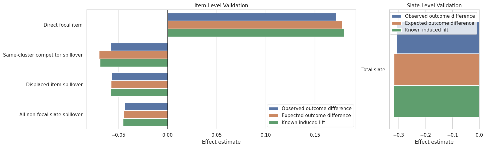
10. Plot Estimated Effects Versus Known Lift

This plot compares observed, expected, and known-lift estimates for each contrast. It is a useful simulation diagnostic: the observed estimates should be directionally consistent with the expected and known-lift signals, even if sampling noise creates some differences.

validation_plot_rows = []
for _, row in validation_table.iterrows():
    if row["contrast"] == "Total slate":
        metrics = {
            "Observed outcome difference": row.get("observed_total_click_diff"),
            "Expected outcome difference": row.get("expected_total_click_diff"),
            "Known induced lift": row.get("known_total_probability_lift_diff"),
        }
    else:
        metrics = {
            "Observed outcome difference": row.get("observed_item_click_diff"),
            "Expected outcome difference": row.get("expected_item_probability_diff"),
            "Known induced lift": row.get("known_item_probability_lift_diff"),
        }
    for metric, value in metrics.items():
        validation_plot_rows.append({"contrast": row["contrast"], "metric": metric, "estimate": value})
validation_plot_df = pd.DataFrame(validation_plot_rows).dropna()

fig, axes = plt.subplots(1, 2, figsize=(16, 5), gridspec_kw={"width_ratios": [3, 1]})

sns.barplot(
    data=validation_plot_df.query("contrast != 'Total slate'"),
    y="contrast",
    x="estimate",
    hue="metric",
    ax=axes[0],
)
axes[0].axvline(0, color="black", linewidth=1)
axes[0].set_title("Item-Level Validation")
axes[0].set_xlabel("Effect estimate")
axes[0].set_ylabel("")
axes[0].legend(title="")

sns.barplot(
    data=validation_plot_df.query("contrast == 'Total slate'"),
    y="contrast",
    x="estimate",
    hue="metric",
    ax=axes[1],
)
axes[1].axvline(0, color="black", linewidth=1)
axes[1].set_title("Slate-Level Validation")
axes[1].set_xlabel("Effect estimate")
axes[1].set_ylabel("")
axes[1].legend(title="")

plt.tight_layout()
fig.savefig(FIGURE_DIR / "12_estimates_vs_known_lift.png", dpi=160, bbox_inches="tight")
plt.show()

The validation view is the honest bridge between simulation and estimation. It tells us whether the estimator recovers the direction and approximate magnitude of the mechanism we built into the data. Later notebooks can use this as a baseline before moving into formal direct/indirect decomposition.

11. Naive Versus Clustered Standard Errors

A common mistake in interference settings is to treat item rows as independent even though treatment is assigned to a whole slate. This cell compares naive and cluster-robust standard errors for the observed-outcome estimates.

se_comparison = observed_estimates[
    [
        "contrast",
        "outcome",
        "estimate",
        "naive_se",
        "cluster_se",
        "cluster_to_naive_se_ratio",
        "clusters",
    ]
].copy()
se_comparison["cluster_minus_naive_se"] = se_comparison["cluster_se"] - se_comparison["naive_se"]
se_comparison = se_comparison.sort_values("cluster_to_naive_se_ratio", ascending=False)

display(se_comparison)
contrast outcome estimate naive_se cluster_se cluster_to_naive_se_ratio clusters cluster_minus_naive_se
9 All non-focal slate spillover Observed simulated click -0.0436 0.0043 0.0046 1.0635 3000 0.0003
6 Displaced-item spillover Observed simulated click -0.0568 0.0054 0.0057 1.0419 3000 0.0002
3 Same-cluster competitor spillover Observed simulated click -0.0577 0.0083 0.0084 1.0107 2456 0.0001
12 Total slate Observed total simulated clicks -0.3078 0.0538 0.0538 1.0001 3000 0.0000
0 Direct focal item Observed simulated click 0.1716 0.0157 0.0157 0.9992 3000 -0.0000

If the cluster standard error is meaningfully different from the naive standard error, that is a warning that row-level uncertainty is not appropriate. Even when the estimates are simple, the uncertainty calculation should match the randomized design.

12. Cluster Bootstrap for Main Observed Effects

The cluster-robust regression standard errors are analytic. This cell adds a cluster bootstrap, resampling slates with replacement and recomputing the treated-control mean difference. The bootstrap is slower but useful as a second uncertainty check.

BOOTSTRAP_REPS = 500
BOOTSTRAP_SEED = 20260428

bootstrap_jobs = [
    ("Direct focal item", focal_rows, "simulated_click"),
    ("Same-cluster competitor spillover", same_cluster_candidates, "simulated_click"),
    ("Displaced-item spillover", would_be_displaced_candidates, "simulated_click"),
    ("All non-focal slate spillover", non_focal_rows, "simulated_click"),
    ("Total slate", slate_outcomes, "total_simulated_clicks"),
]

bootstrap_rows = []
bootstrap_summaries = []
for i, (contrast, df, outcome) in enumerate(bootstrap_jobs):
    estimates = cluster_bootstrap_difference(
        df,
        outcome=outcome,
        treatment="promotion_applied",
        cluster_col="slate_id",
        n_bootstrap=BOOTSTRAP_REPS,
        seed=BOOTSTRAP_SEED + i,
    )
    estimates = estimates[~np.isnan(estimates)]
    for draw_id, estimate in enumerate(estimates):
        bootstrap_rows.append(
            {
                "contrast": contrast,
                "outcome": outcome,
                "bootstrap_draw": draw_id,
                "estimate": estimate,
            }
        )
    bootstrap_summaries.append(
        {
            "contrast": contrast,
            "outcome": outcome,
            "bootstrap_draws": len(estimates),
            "bootstrap_mean": estimates.mean(),
            "bootstrap_se": estimates.std(ddof=1),
            "bootstrap_ci_95_lower": np.quantile(estimates, 0.025),
            "bootstrap_ci_95_upper": np.quantile(estimates, 0.975),
        }
    )

bootstrap_distribution = pd.DataFrame(bootstrap_rows)
bootstrap_summary = pd.DataFrame(bootstrap_summaries)

display(bootstrap_summary)
contrast outcome bootstrap_draws bootstrap_mean bootstrap_se bootstrap_ci_95_lower bootstrap_ci_95_upper
0 Direct focal item simulated_click 500 0.1712 0.0161 0.1383 0.2015
1 Same-cluster competitor spillover simulated_click 500 -0.0578 0.0083 -0.0733 -0.0420
2 Displaced-item spillover simulated_click 500 -0.0565 0.0061 -0.0686 -0.0449
3 All non-focal slate spillover simulated_click 500 -0.0438 0.0047 -0.0524 -0.0343
4 Total slate total_simulated_clicks 500 -0.3055 0.0536 -0.4169 -0.2042

The bootstrap intervals should usually tell the same qualitative story as the cluster-robust intervals. If they disagree sharply, that would be a sign to inspect skew, leverage, or sparse treated/control support within a contrast.

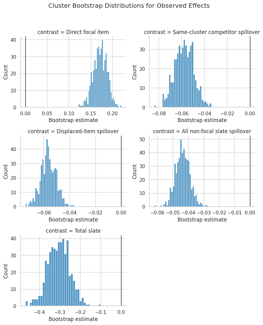
13. Plot Bootstrap Distributions

This plot shows the cluster bootstrap distribution for each observed effect. The vertical line marks zero, making it easy to see whether the bootstrap mass is mostly positive, mostly negative, or centered near no effect.

g = sns.FacetGrid(
    bootstrap_distribution,
    col="contrast",
    col_wrap=2,
    sharex=False,
    sharey=False,
    height=3.4,
    aspect=1.25,
)
g.map_dataframe(sns.histplot, x="estimate", bins=35, color="tab:blue")
for ax in g.axes.flat:
    ax.axvline(0, color="black", linewidth=1)
    ax.set_xlabel("Bootstrap estimate")
g.fig.suptitle("Cluster Bootstrap Distributions for Observed Effects", y=1.03)
plt.tight_layout()
g.fig.savefig(FIGURE_DIR / "13_cluster_bootstrap_distributions.png", dpi=160, bbox_inches="tight")
plt.show()

The bootstrap plots add shape information that a table cannot show. For example, slate-level total effects can have a wider distribution because total clicks aggregate many item outcomes and because displacement varies by focal position and cluster composition.

14. Decompose the Total Slate Effect

The total slate effect combines focal gains and competitor losses. This cell uses the known expected lift components from the simulation to decompose promoted slates into direct focal lift, same-cluster spillover loss, other-spillover loss, and net total lift.

This is not the final formal decomposition notebook yet. It is a diagnostic showing why the total effect can differ from the direct effect.

promoted_slates = slate_outcomes.query("promotion_applied == 1").copy()

direct_component = promoted_slates["direct_expected_lift"].mean()
slate_decomposition = pd.DataFrame(
    {
        "component": [
            "Direct focal expected lift",
            "Same-cluster spillover expected lift",
            "Other spillover expected lift",
            "Net total expected lift",
        ],
        "mean_lift_per_promoted_slate": [
            direct_component,
            promoted_slates["same_cluster_spillover_expected_lift"].mean(),
            promoted_slates["other_spillover_expected_lift"].mean(),
            promoted_slates["total_known_probability_lift"].mean(),
        ],
    }
)
slate_decomposition["share_of_direct_gain_magnitude"] = (
    slate_decomposition["mean_lift_per_promoted_slate"] / abs(direct_component)
)

display(slate_decomposition)
component mean_lift_per_promoted_slate share_of_direct_gain_magnitude
0 Direct focal expected lift 0.1794 1.0000
1 Same-cluster spillover expected lift -0.1965 -1.0953
2 Other spillover expected lift -0.3010 -1.6777
3 Net total expected lift -0.3180 -1.7730

The decomposition is the core product lesson of this interference project. Looking only at the promoted item can make an intervention look good, while the net slate effect can be weaker or negative once substitute and displaced-item losses are counted.

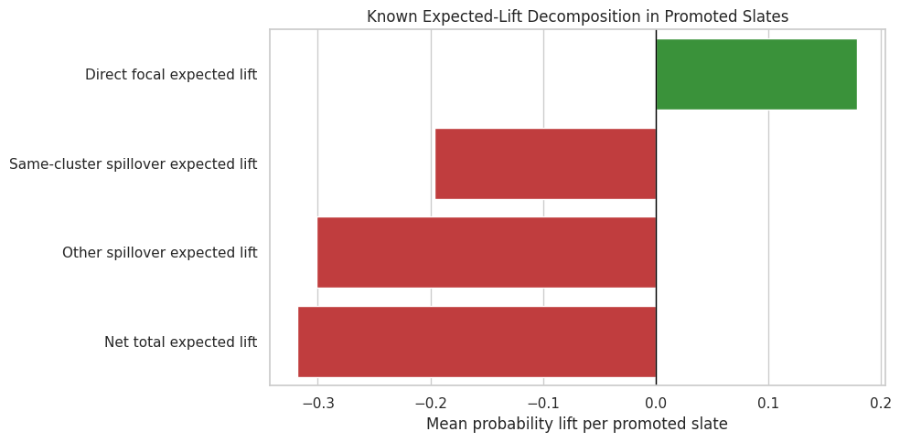
15. Plot the Total Effect Decomposition

This plot turns the decomposition into a report-friendly figure. Positive bars represent focal gains, while negative bars represent spillover losses. The net bar summarizes the slate-level consequence.

fig, ax = plt.subplots(figsize=(10, 5))
colors = ["tab:green" if value >= 0 else "tab:red" for value in slate_decomposition["mean_lift_per_promoted_slate"]]
sns.barplot(
    data=slate_decomposition,
    x="mean_lift_per_promoted_slate",
    y="component",
    hue="component",
    palette=dict(zip(slate_decomposition["component"], colors)),
    legend=False,
    ax=ax,
)
ax.axvline(0, color="black", linewidth=1)
ax.set_title("Known Expected-Lift Decomposition in Promoted Slates")
ax.set_xlabel("Mean probability lift per promoted slate")
ax.set_ylabel("")
plt.tight_layout()
fig.savefig(FIGURE_DIR / "14_total_effect_decomposition.png", dpi=160, bbox_inches="tight")
plt.show()

This figure explains why interference changes the evaluation question. The promoted item is only one part of the slate. A good recommender evaluation should ask whether the whole slate, cluster, or user session improved after accounting for displaced attention.

16. Cluster-Level Effect Heterogeneity

Spillovers may differ by genre cluster. This cell estimates observed direct focal effects and same-cluster spillover effects for clusters with enough support. These estimates are exploratory; the goal is to see where the simulated mechanism is strongest and where data are too sparse.

MIN_CLUSTER_ARM_ROWS = 30
cluster_effect_rows = []

for cluster, df in focal_rows.groupby("focal_spillover_cluster"):
    treated_n = int(df["promotion_applied"].sum())
    control_n = int((1 - df["promotion_applied"]).sum())
    if treated_n >= MIN_CLUSTER_ARM_ROWS and control_n >= MIN_CLUSTER_ARM_ROWS:
        result = difference_in_means(
            df,
            outcome="simulated_click",
            treatment="promotion_applied",
            cluster_col="slate_id",
            contrast_name="Direct focal item",
            outcome_label="Observed simulated click",
        )
        result["cluster"] = cluster
        result["effect_family"] = "direct"
        cluster_effect_rows.append(result)

for cluster, df in same_cluster_candidates.groupby("focal_spillover_cluster"):
    treated_n = int(df["promotion_applied"].sum())
    control_n = int((1 - df["promotion_applied"]).sum())
    if treated_n >= MIN_CLUSTER_ARM_ROWS and control_n >= MIN_CLUSTER_ARM_ROWS:
        result = difference_in_means(
            df,
            outcome="simulated_click",
            treatment="promotion_applied",
            cluster_col="slate_id",
            contrast_name="Same-cluster competitor spillover",
            outcome_label="Observed simulated click",
        )
        result["cluster"] = cluster
        result["effect_family"] = "same_cluster_spillover"
        cluster_effect_rows.append(result)

cluster_effects = pd.DataFrame(cluster_effect_rows)
cluster_effects = cluster_effects.sort_values(["effect_family", "estimate"])

display(cluster_effects[
    [
        "effect_family",
        "cluster",
        "estimate",
        "cluster_se",
        "ci_95_lower",
        "ci_95_upper",
        "treated_n",
        "control_n",
        "clusters",
    ]
])
effect_family cluster estimate cluster_se ci_95_lower ci_95_upper treated_n control_n clusters
6 direct Horror 0.0787 0.0981 -0.1135 0.2710 31 34 65
5 direct Drama 0.1179 0.0339 0.0514 0.1844 317 319 636
0 direct Action 0.1659 0.0298 0.1074 0.2243 401 398 799
4 direct Crime 0.1660 0.0560 0.0563 0.2757 130 123 253
3 direct Comedy 0.1924 0.0334 0.1269 0.2578 338 320 658
1 direct Adventure 0.2329 0.0483 0.1382 0.3275 168 150 318
2 direct Animation 0.3372 0.1054 0.1306 0.5437 32 38 70
9 same_cluster_spillover Animation -0.1957 0.0852 -0.3627 -0.0288 32 38 35
8 same_cluster_spillover Adventure -0.0847 0.0350 -0.1532 -0.0162 282 226 219
12 same_cluster_spillover Drama -0.0753 0.0179 -0.1105 -0.0402 974 1012 587
7 same_cluster_spillover Action -0.0499 0.0136 -0.0765 -0.0233 1692 1591 759
10 same_cluster_spillover Comedy -0.0482 0.0158 -0.0792 -0.0171 1092 1011 606
11 same_cluster_spillover Crime -0.0391 0.0452 -0.1276 0.0494 165 184 165

The cluster-level table is exploratory, not the main causal result. It helps identify where direct gains or spillover losses may be concentrated. Sparse clusters are filtered out so the table stays focused on segments with enough treated and control support.

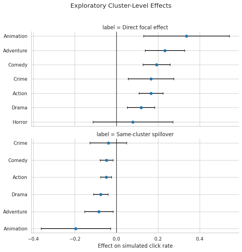
17. Plot Cluster-Level Direct and Spillover Effects

This plot shows the exploratory cluster effects with intervals. It is useful for seeing whether some content groups are more displacement-prone than others.

if not cluster_effects.empty:
    plot_cluster_effects = cluster_effects.copy()
    plot_cluster_effects["label"] = plot_cluster_effects["effect_family"].map(
        {
            "direct": "Direct focal effect",
            "same_cluster_spillover": "Same-cluster spillover",
        }
    )

    g = sns.FacetGrid(
        plot_cluster_effects,
        row="label",
        sharex=True,
        sharey=False,
        height=4.0,
        aspect=2.0,
    )

    def point_ci(data, **kwargs):
        ax = plt.gca()
        ordered = data.sort_values("estimate")
        y_positions = np.arange(len(ordered))
        ax.errorbar(
            x=ordered["estimate"],
            y=y_positions,
            xerr=[
                ordered["estimate"] - ordered["ci_95_lower"],
                ordered["ci_95_upper"] - ordered["estimate"],
            ],
            fmt="o",
            color="tab:blue",
            ecolor="black",
            capsize=3,
        )
        ax.set_yticks(y_positions)
        ax.set_yticklabels(ordered["cluster"])
        ax.axvline(0, color="black", linewidth=1)
        ax.set_xlabel("Effect on simulated click rate")
        ax.set_ylabel("")

    g.map_dataframe(point_ci)
    g.fig.suptitle("Exploratory Cluster-Level Effects", y=1.02)
    plt.tight_layout()
    g.fig.savefig(FIGURE_DIR / "15_cluster_level_effects.png", dpi=160, bbox_inches="tight")
    plt.show()
else:
    print("No clusters met the minimum support threshold.")

The cluster plot should be read as a guide for deeper analysis rather than a final segmentation claim. Later notebooks can formalize these ideas by decomposing effects and checking sensitivity to the spillover exposure definition.

18. Save Estimation Artifacts

This cell saves the main estimate table, observed-outcome summary, bootstrap distribution, bootstrap summary, validation table, decomposition table, and exploratory cluster effects. These artifacts let the next notebook focus on formal direct/indirect/total decomposition without recomputing the basic randomized estimators.

ESTIMATE_OUTPUT = PROCESSED_DIR / "movielens_interference_cluster_estimates.csv"
OBSERVED_OUTPUT = PROCESSED_DIR / "movielens_interference_observed_effects.csv"
VALIDATION_OUTPUT = PROCESSED_DIR / "movielens_interference_estimator_validation.csv"
BOOTSTRAP_OUTPUT = PROCESSED_DIR / "movielens_interference_cluster_bootstrap.csv"
BOOTSTRAP_SUMMARY_OUTPUT = PROCESSED_DIR / "movielens_interference_cluster_bootstrap_summary.csv"
DECOMPOSITION_OUTPUT = PROCESSED_DIR / "movielens_interference_slate_decomposition.csv"
CLUSTER_EFFECT_OUTPUT = PROCESSED_DIR / "movielens_interference_cluster_effects.csv"

estimate_table.to_csv(ESTIMATE_OUTPUT, index=False)
observed_estimates.to_csv(OBSERVED_OUTPUT, index=False)
validation_table.to_csv(VALIDATION_OUTPUT, index=False)
bootstrap_distribution.to_csv(BOOTSTRAP_OUTPUT, index=False)
bootstrap_summary.to_csv(BOOTSTRAP_SUMMARY_OUTPUT, index=False)
slate_decomposition.to_csv(DECOMPOSITION_OUTPUT, index=False)
cluster_effects.to_csv(CLUSTER_EFFECT_OUTPUT, index=False)

saved_outputs = pd.DataFrame(
    {
        "artifact": [
            "all_cluster_estimates",
            "observed_effects",
            "estimator_validation",
            "cluster_bootstrap_distribution",
            "cluster_bootstrap_summary",
            "slate_decomposition",
            "cluster_effects",
        ],
        "path": [
            str(ESTIMATE_OUTPUT),
            str(OBSERVED_OUTPUT),
            str(VALIDATION_OUTPUT),
            str(BOOTSTRAP_OUTPUT),
            str(BOOTSTRAP_SUMMARY_OUTPUT),
            str(DECOMPOSITION_OUTPUT),
            str(CLUSTER_EFFECT_OUTPUT),
        ],
    }
)

display(saved_outputs)
artifact path
0 all_cluster_estimates /home/apex/Documents/ranking_sys/data/processe...
1 observed_effects /home/apex/Documents/ranking_sys/data/processe...
2 estimator_validation /home/apex/Documents/ranking_sys/data/processe...
3 cluster_bootstrap_distribution /home/apex/Documents/ranking_sys/data/processe...
4 cluster_bootstrap_summary /home/apex/Documents/ranking_sys/data/processe...
5 slate_decomposition /home/apex/Documents/ranking_sys/data/processe...
6 cluster_effects /home/apex/Documents/ranking_sys/data/processe...

The saved files are the handoff to the next notebook. The most important tables are the observed effects, the validation table, and the slate decomposition. Together they show the estimated promoted-item gain, the estimated spillover loss, and the net slate consequence.

19. Notebook Takeaways

This notebook estimated the randomized promotion simulation from several angles:

  • The direct focal-item effect measures the gain from moving a lower-ranked movie to the top of a slate.
  • Same-cluster and displaced-item contrasts measure competitor losses caused by the same promotion.
  • The total slate effect measures the net product outcome after combining focal gains and spillover losses.
  • Clustered uncertainty is the right default because promotion is assigned at the slate level.
  • The known simulation signal confirms why interference matters: a direct gain can coexist with a weaker or negative total slate effect.

The next notebook should formalize the decomposition into direct, indirect, and total effects, then compare alternative exposure definitions such as same-slate spillover, same-cluster spillover, and displaced-position spillover.