This notebook turns the MovieLens seed slates from the setup notebook into a causal simulation dataset for studying interference and spillovers.
The key idea is simple: recommendation items in the same slate compete for limited attention. If one lower-ranked movie is promoted to the top of a slate, the promoted movie may gain visibility, but other movies can lose visibility or attention. The strongest spillover should usually fall on nearby substitute items, such as movies in the same genre cluster.
This notebook does not estimate causal effects yet. Instead, it defines the experimental structure that later estimators will use:
the item-row unit of analysis,
the slate-level randomized promotion assignment,
direct treatment exposure for promoted focal movies,
spillover exposure for non-promoted movies in the same slate,
stronger same-cluster spillover exposure for substitute movies,
simulated post-promotion outcomes based on relevance, visibility, and competition.
The result is an analysis-ready table with known assignment probabilities. That matters because the later notebooks can estimate direct, indirect, and total effects while clearly explaining what is randomized and what is simulated.
1. Environment and Paths
This cell imports the libraries used in the notebook and finds the repository root by searching upward for the processed MovieLens files. This makes the notebook work whether it is run from the repository root, from JupyterLab, or through nbconvert.
from pathlib import Pathimport matplotlib.pyplot as pltimport numpy as npimport pandas as pdimport seaborn as snsfrom IPython.display import displaysns.set_theme(style="whitegrid", context="notebook")pd.set_option("display.max_columns", 100)pd.set_option("display.max_rows", 80)pd.set_option("display.float_format", lambda value: f"{value:,.4f}")candidate_roots = [Path.cwd(), *Path.cwd().parents]PROJECT_DIR =next( root for root in candidate_rootsif (root /"data"/"processed"/"movielens_interference_slate_seed.parquet").exists())PROCESSED_DIR = PROJECT_DIR /"data"/"processed"NOTEBOOK_DIR = PROJECT_DIR /"notebooks"/"interference_spillover_effects"WRITEUP_DIR = NOTEBOOK_DIR /"writeup"FIGURE_DIR = WRITEUP_DIR /"figures"TABLE_DIR = WRITEUP_DIR /"tables"FIGURE_DIR.mkdir(parents=True, exist_ok=True)TABLE_DIR.mkdir(parents=True, exist_ok=True)SLATE_SEED_PATH = PROCESSED_DIR /"movielens_interference_slate_seed.parquet"ITEMS_PATH = PROCESSED_DIR /"movielens_interference_items.parquet"USERS_PATH = PROCESSED_DIR /"movielens_interference_user_features.parquet"SLATE_SEED_PATH.exists(), ITEMS_PATH.exists(), USERS_PATH.exists()
(True, True, True)
All three checks should return True. These are the processed outputs from the setup notebook: seed slates, item features, and user features. This notebook uses those files as fixed inputs so the exposure mapping is reproducible.
2. Load the Seed Slates and Feature Tables
The seed slate table contains one row per user-slate-movie candidate. It already has a seed position, observed relevance from the user’s rating, and a genre-based spillover cluster. This cell loads the seed table and attaches user and item features that will be useful for balance checks and outcome simulation.
The loaded table should still have complete slates of equal size. Equal slate size keeps the simulation easy to explain: each promotion happens inside a 12-item candidate slate, and every slate has the same amount of attention to allocate.
3. Define the Randomized Promotion Design
This cell defines the randomized intervention. In each slate, one focal movie is selected from the lower-ranked positions, then the slate is randomized to either promote that focal movie or leave the slate unchanged.
The design has two stages:
Focal selection: choose one eligible lower-position movie from each slate. This creates a candidate item that could be promoted.
Promotion assignment: flip a randomized promotion flag with probability 0.5. If assigned, the focal movie moves to position 1 and earlier items shift down by one position.
This design creates a clean comparison between promoted and non-promoted focal movies while also generating spillover exposure for the other items in promoted slates.
The observed promotion rate should be close to 50 percent. The focal items come from lower positions, which makes the intervention meaningful: moving a movie from position 5 or below into the top position creates a visible change and forces other items to shift.
4. Check Randomization Balance for Focal Items
Because promotion is randomized after focal selection, promoted and non-promoted focal items should look similar before treatment. This cell compares focal relevance, focal position, and user/item features across the two assignment arms. Large differences would suggest a coding problem rather than a real causal pattern.
The balance table is a pre-estimation diagnostic. Since assignment is random, small differences are expected by chance, but systematic differences should be limited. Later effect estimates can therefore lean on the randomized design rather than heavy covariate adjustment.
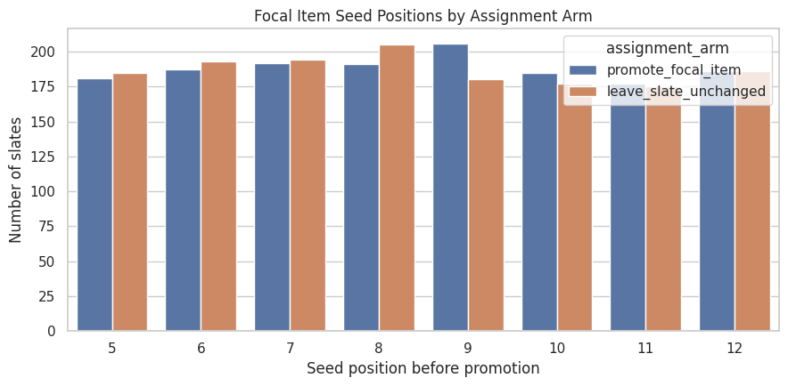
5. Visualize Focal Position Assignment
The focal item is always chosen from lower seed positions. This plot shows whether focal selection is spread across eligible positions or concentrated in one area of the slate. A spread is useful because promotion creates a range of position changes.
fig, ax = plt.subplots(figsize=(9, 4.5))sns.countplot(data=focal_items, x="focal_seed_position", hue="assignment_arm", ax=ax)ax.set_title("Focal Item Seed Positions by Assignment Arm")ax.set_xlabel("Seed position before promotion")ax.set_ylabel("Number of slates")plt.tight_layout()fig.savefig(FIGURE_DIR /"06_focal_position_assignment.png", dpi=160, bbox_inches="tight")plt.show()
The assignment arms should have similar focal-position distributions. This matters because position gain is the mechanism of the direct effect. If one arm had much deeper focal items, promoted and control slates would not be comparable in a clean way.
6. Map Direct and Spillover Exposures
This cell joins the slate-level assignment back to every item row and creates the core exposure variables.
Key variables:
direct_treatment: the row is the focal item and its slate was promoted.
same_slate_spillover: another item in the same slate was promoted.
same_cluster_spillover: a non-focal item shares the promoted focal item’s spillover cluster.
displaced_by_promotion: a non-focal item was above the focal item and shifted down after promotion.
final_position: the row’s post-assignment position.
visibility_gain: change in a simple visibility score after promotion.
The exposure groups make the interference structure explicit. The promoted focal item is the direct-treatment unit. Non-focal items in promoted slates are spillover-exposed, and same-cluster non-focal items are the most important substitute group. The final-position validity check confirms that each slate still has positions 1 through 12 after the simulated promotion.
7. Summarize Exposure Group Shares
This cell converts exposure counts into shares. The counts are useful, but shares make it easier to see how much data is available for each causal contrast. Same-cluster spillover rows are especially important because they represent plausible substitute displacement.
The direct-treatment group is small by design because each promoted slate has one promoted focal item. Spillover groups are larger because every other item in a promoted slate can be affected. This asymmetry is exactly why item-level analyses can be misleading if they only count the promoted item’s gain.
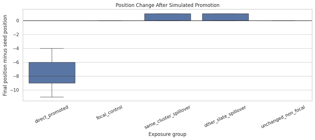
8. Plot Position Changes by Exposure Group
Promotion changes the focal item’s position dramatically and shifts some other items down. This plot shows the distribution of position changes. Negative values mean a movie moved upward; positive values mean it moved downward.
plot_order = ["direct_promoted","focal_control","same_cluster_spillover","other_slate_spillover","unchanged_non_focal",]fig, ax = plt.subplots(figsize=(11, 5))sns.boxplot( data=exposure, x="exposure_group", y="position_change", order=plot_order, ax=ax, showfliers=False,)ax.axhline(0, color="black", linewidth=1)ax.set_title("Position Change After Simulated Promotion")ax.set_xlabel("Exposure group")ax.set_ylabel("Final position minus seed position")ax.tick_params(axis="x", rotation=25)plt.tight_layout()fig.savefig(FIGURE_DIR /"07_position_change_by_exposure_group.png", dpi=160, bbox_inches="tight")plt.show()
The plot should show a strong upward move for directly promoted focal items and downward movement for displaced non-focal items. This is the mechanical source of interference: promotion does not simply add attention to one item; it reallocates attention within the slate.
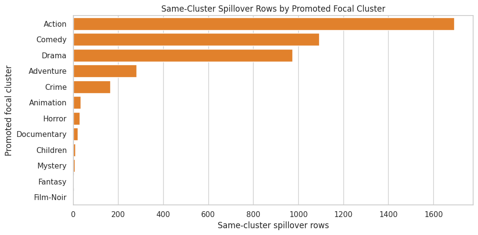
9. Same-Cluster Spillover by Genre Cluster
Same-cluster spillover is not evenly distributed across genres. This cell summarizes how often each spillover cluster appears as the promoted focal cluster and how many same-cluster competitors are exposed. This helps identify where later spillover estimates will have enough support.
Clusters with more same-cluster spillover rows will support more stable indirect-effect estimates. Sparse clusters can still be included in overall estimates, but later segment-level reporting should avoid over-interpreting very small groups.
10. Plot Same-Cluster Spillover Volume
This plot focuses on the largest promoted focal clusters. It shows where substitute displacement is most observable in the simulated data.
The largest clusters are the best candidates for detailed spillover analysis. This is also a product-relevant view: substitution is easier to reason about when the promoted item and competing items are in the same content family.
11. Simulate Observed Outcomes Under Competition
The seed ratings tell us user-item relevance, but they are not post-promotion outcomes. This cell creates simulated binary engagement outcomes using a transparent data-generating process.
The simulated click probability depends on:
user-item relevance from the observed rating,
baseline user rating tendency,
item popularity and liked rate,
final visibility after promotion,
a positive direct boost for promoted focal items,
a small generic attention penalty for non-focal items in promoted slates,
a stronger penalty for same-cluster substitutes.
The exact outcome model is synthetic, but the assumptions are explicit. That is the right setup for this interference notebook because MovieLens does not contain real randomized exposure logs.
The simulated outcome table should show positive probability lift for directly promoted items and negative or near-negative lift for spillover groups. This is by design: the notebook is creating a controlled environment where later estimators should recover both promoted-item gains and competitor displacement.
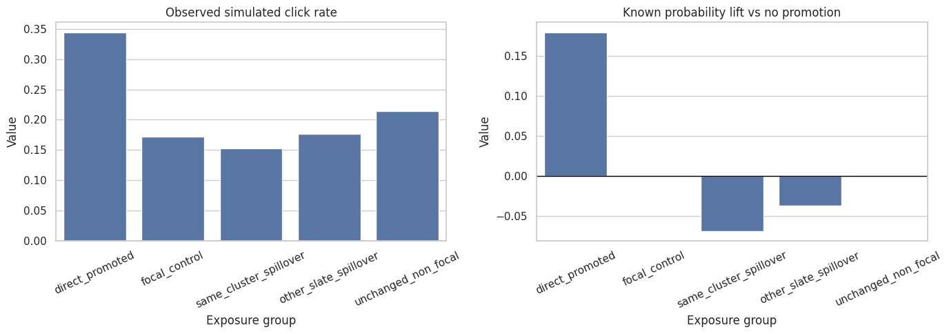
12. Plot Simulated Outcomes by Exposure Group
This plot compares simulated click rates and known probability lift across exposure groups. It is not a causal estimate yet; it is a sanity check that the simulated data-generating process creates the expected pattern.
The left panel reflects both relevance selection and exposure, while the right panel isolates the known probability change induced by the simulation. This distinction is important: raw click-rate differences are not the same as causal effects, even in a randomized simulation, because groups can differ in baseline relevance and position.
13. Build Slate-Level Outcomes
Interference is often best evaluated at the slate level because one item’s gain can be another item’s loss. This cell aggregates item-row outcomes into slate-level totals and separates focal, same-cluster competitor, and other competitor components.
The slate-level table is where displacement becomes visible. A promoted focal item can have a positive direct expected lift, while same-cluster and other competitors can have negative expected lifts. The total slate lift is the net product-relevant quantity.
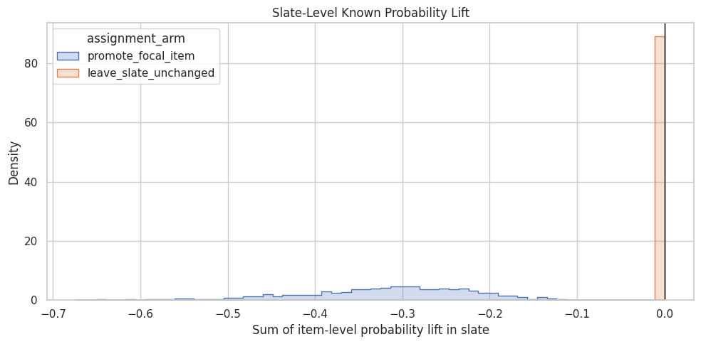
14. Plot Slate-Level Net Lift
This plot shows the distribution of known expected total lift at the slate level. The promoted arm should have non-zero lift by construction, while the control arm should be zero because no slate positions changed.
fig, ax = plt.subplots(figsize=(10, 5))sns.histplot( data=slate_outcomes, x="total_known_probability_lift", hue="assignment_arm", bins=60, element="step", stat="density", common_norm=False, ax=ax,)ax.axvline(0, color="black", linewidth=1)ax.set_title("Slate-Level Known Probability Lift")ax.set_xlabel("Sum of item-level probability lift in slate")ax.set_ylabel("Density")plt.tight_layout()fig.savefig(FIGURE_DIR /"10_slate_level_known_lift.png", dpi=160, bbox_inches="tight")plt.show()
This distribution shows why total effects matter. A promotion can be beneficial for the focal item but still have a muted or negative net slate effect if competitor displacement is large. Later notebooks will estimate this net effect from observed simulated outcomes.
15. Create a Compact Causal Design Summary
This cell summarizes the design choices and readiness checks in a compact table. The goal is to make the assumptions visible before any estimator is applied.
readiness_checks = pd.DataFrame( [ {"check": "complete_seed_slates_loaded","value": exposure["slate_id"].nunique(),"notes": "Each slate contains 12 item rows from the setup notebook.", }, {"check": "promotion_probability","value": PROMOTION_PROBABILITY,"notes": "Slate-level randomized assignment probability after focal selection.", }, {"check": "observed_promotion_rate","value": exposure.drop_duplicates("slate_id")["promotion_applied"].mean(),"notes": "Should be close to the design probability.", }, {"check": "direct_treatment_rows","value": int(exposure["direct_treatment"].sum()),"notes": "One directly treated focal item per promoted slate.", }, {"check": "same_slate_spillover_rows","value": int(exposure["same_slate_spillover"].sum()),"notes": "Non-focal items in promoted slates.", }, {"check": "same_cluster_spillover_rows","value": int(exposure["same_cluster_spillover"].sum()),"notes": "Non-focal items sharing the promoted focal item's cluster.", }, {"check": "invalid_final_position_slates","value": len(invalid_position_slates),"notes": "Should be zero; each slate should keep positions 1 through 12.", }, {"check": "mean_promoted_slate_known_lift","value": slate_outcomes.query("promotion_applied == 1")["total_known_probability_lift"].mean(),"notes": "Average known net expected lift in promoted slates under the simulation.", }, ])display(readiness_checks)
check
value
notes
0
complete_seed_slates_loaded
3,000.0000
Each slate contains 12 item rows from the setu...
1
promotion_probability
0.5000
Slate-level randomized assignment probability ...
2
observed_promotion_rate
0.5017
Should be close to the design probability.
3
direct_treatment_rows
1,505.0000
One directly treated focal item per promoted s...
4
same_slate_spillover_rows
16,555.0000
Non-focal items in promoted slates.
5
same_cluster_spillover_rows
4,309.0000
Non-focal items sharing the promoted focal ite...
6
invalid_final_position_slates
0.0000
Should be zero; each slate should keep positio...
7
mean_promoted_slate_known_lift
-0.3180
Average known net expected lift in promoted sl...
The readiness table is a contract for the next notebook. It says how many direct and spillover observations exist, verifies valid final positions, and records the known assignment probability. Estimation notebooks should use these diagnostics before reporting causal results.
16. Save the Exposure Mapping Artifacts
This cell saves the item-row exposure mapping, slate-level outcomes, focal assignment table, and diagnostic summaries. Later notebooks can load these files directly and focus on estimation rather than rebuilding the simulation.
The saved exposure mapping is the main output of this notebook. It contains treatment, spillover, position, visibility, simulated outcome, and assignment variables at the item-row level. That table is ready for direct-effect and spillover-effect estimators.
17. Notebook Takeaways
This notebook converted MovieLens seed slates into a randomized interference simulation:
One eligible lower-ranked focal item was selected in each slate.
Slates were randomized to promote the focal item or leave the slate unchanged.
Direct treatment, same-slate spillover, same-cluster spillover, displacement, and final position were explicitly mapped.
Simulated outcomes were generated from relevance, visibility, and competition assumptions.
Item-level and slate-level outputs were saved for the next estimation notebook.
The next notebook should estimate direct, spillover, and total effects using the randomized assignment. A natural next step is 03_cluster_randomized_estimators.ipynb, which can compare simple difference-in-means estimators, cluster-robust standard errors, and slate-level total-effect estimates.