MovieLens Interference Setup and EDA

This notebook starts the interference and spillover effects analysis. The causal problem is different from standard treatment-effect estimation because recommendation items compete with one another. If one movie is promoted into a visible slate position, another movie may lose visibility, attention, clicks, ratings, or watch time. That means an item’s outcome may depend not only on its own treatment status, but also on the treatment assignments of other nearby items.

The purpose of this first notebook is to understand the MovieLens data and prepare a clean foundation for later spillover notebooks. MovieLens does not contain true production impressions or randomized promotion assignments, so this project will use MovieLens as a realistic preference dataset and then simulate recommendation slates, promotion assignments, and item competition structures.

Dataset Field Guide

MovieLens 32M is distributed as four main CSV files inside ml-32m.zip.

ratings.csv

Each row is a user-movie rating event.

  • userId: anonymized user identifier. A user can rate many movies.
  • movieId: MovieLens movie identifier. This links to movies.csv, links.csv, and tags.csv.
  • rating: explicit star rating on a 0.5 to 5.0 scale. In this project it is a preference signal, not a direct exposure or click outcome.
  • timestamp: Unix timestamp for when the rating was created. This lets us study recency, user histories, and time ordering.

movies.csv

Each row is a movie catalog item.

  • movieId: MovieLens movie identifier.
  • title: movie title, usually with a release year in parentheses.
  • genres: pipe-delimited genre string such as Comedy|Romance. A movie can belong to multiple genres. We will use genres to create substitute groups because movies in similar genres plausibly compete for user attention.

tags.csv

Each row is a user-applied free-text tag for a movie.

  • userId: anonymized user identifier for the tag event.
  • movieId: tagged movie identifier.
  • tag: user-generated text label such as an actor, theme, mood, franchise, or descriptive keyword.
  • timestamp: Unix timestamp for when the tag was applied.

Tags are useful for richer item similarity, but they are sparse and noisy. In this first notebook we use them mainly for understanding catalog semantics.

links.csv

Each row maps a MovieLens movie to external identifiers.

  • movieId: MovieLens movie identifier.
  • imdbId: IMDb identifier.
  • tmdbId: TMDb identifier.

This project does not need external metadata immediately, but the file is useful if we later want posters, richer genres, cast, crew, or production metadata.

Causal Setup Preview

Later notebooks will convert this preference dataset into a simulated recommendation setting:

  • A slate is a set of movies shown together to a user.
  • A treated item is a movie promoted into a more visible position in the slate.
  • A spillover-exposed item is another item in the same slate, especially a similar or substitutable movie.
  • A direct effect measures what happens to the promoted item.
  • An indirect or spillover effect measures what happens to competing items.
  • A total effect combines promoted-item gains and displaced-item losses at the slate or cluster level.

This notebook does not estimate those effects yet. It builds the data understanding and processed inputs needed to do that carefully.

1. Environment and Paths

This cell imports the libraries used for dataset inspection, plotting, and processed-data export. It also defines paths to the MovieLens zip file and the processed-data folder. The notebook reads directly from the zip file so we do not need to permanently extract a very large dataset into the repository.

from pathlib import Path
from zipfile import ZipFile

import matplotlib.pyplot as plt
import numpy as np
import pandas as pd
import seaborn as sns
from IPython.display import display

sns.set_theme(style="whitegrid", context="notebook")
pd.set_option("display.max_columns", 80)
pd.set_option("display.max_rows", 60)
pd.set_option("display.float_format", lambda value: f"{value:,.4f}")

candidate_roots = [Path.cwd(), *Path.cwd().parents]
PROJECT_DIR = next(
    root for root in candidate_roots
    if (root / "data" / "movieLens" / "ml-32m.zip").exists()
)

DATA_DIR = PROJECT_DIR / "data"
RAW_ZIP = DATA_DIR / "movieLens" / "ml-32m.zip"
PROCESSED_DIR = DATA_DIR / "processed"
PROCESSED_DIR.mkdir(parents=True, exist_ok=True)

NOTEBOOK_DIR = PROJECT_DIR / "notebooks" / "interference_spillover_effects"
WRITEUP_DIR = NOTEBOOK_DIR / "writeup"
FIGURE_DIR = WRITEUP_DIR / "figures"
TABLE_DIR = WRITEUP_DIR / "tables"
FIGURE_DIR.mkdir(parents=True, exist_ok=True)
TABLE_DIR.mkdir(parents=True, exist_ok=True)

RAW_ZIP.exists(), RAW_ZIP
(True, PosixPath('/home/apex/Documents/ranking_sys/data/movieLens/ml-32m.zip'))

The path check should return True. If it does, the notebook has found the compressed MovieLens file and can read the CSVs directly from it. The writeup folders are also created here so later cells can save lightweight tables and figures without scattering files across the project.

2. Inspect the MovieLens Archive

Before loading data, we inspect the zip archive itself. This confirms which files are present, how large they are, and whether the archive matches the standard MovieLens 32M layout. This is a useful first notebook habit because many downstream errors come from assuming a folder layout that differs from the local download.

with ZipFile(RAW_ZIP) as zf:
    archive_rows = []
    for info in zf.infolist():
        if not info.is_dir():
            archive_rows.append(
                {
                    "file": info.filename,
                    "compressed_mb": info.compress_size / 1_000_000,
                    "uncompressed_mb": info.file_size / 1_000_000,
                }
            )

archive_df = pd.DataFrame(archive_rows).sort_values("uncompressed_mb", ascending=False)
display(archive_df)
file compressed_mb uncompressed_mb
4 ml-32m/ratings.csv 218.7859 877.0762
0 ml-32m/tags.csv 17.8637 72.3539
5 ml-32m/movies.csv 1.4578 4.2429
1 ml-32m/links.csv 0.8377 1.9507
2 ml-32m/README.txt 0.0037 0.0092
3 ml-32m/checksums.txt 0.0001 0.0002

The ratings file is by far the largest file, so the rest of the notebook treats it carefully. The movie metadata is small enough to load fully, while ratings need chunked reading and a deterministic user sample. That keeps the EDA reproducible without requiring the notebook to hold all 32 million interactions in memory.

3. Load and Enrich the Movie Catalog

The movie catalog is the natural item table for the interference problem. This cell loads every movie, parses the release year from the title when available, splits the pipe-delimited genre string into a list, and creates a primary genre for simple grouping. Later notebooks can use these genre groups as item clusters where spillovers are most plausible.

with ZipFile(RAW_ZIP) as zf:
    with zf.open("ml-32m/movies.csv") as file:
        movies = pd.read_csv(file)

movies = movies.assign(
    release_year=movies["title"].str.extract(r"\((\d{4})\)\s*$")[0].astype("float"),
    clean_title=movies["title"].str.replace(r"\s*\(\d{4}\)\s*$", "", regex=True),
    genre_list=movies["genres"].fillna("(no genres listed)").str.split("|"),
)
movies["genre_count"] = movies["genre_list"].str.len()
movies["primary_genre"] = movies["genre_list"].str[0]

movie_summary = pd.DataFrame(
    {
        "metric": [
            "movies",
            "movies_with_release_year",
            "movies_without_genres",
            "distinct_primary_genres",
            "median_genres_per_movie",
        ],
        "value": [
            len(movies),
            int(movies["release_year"].notna().sum()),
            int((movies["genres"] == "(no genres listed)").sum()),
            movies["primary_genre"].nunique(),
            movies["genre_count"].median(),
        ],
    }
)

display(movie_summary)
display(movies.head())
metric value
0 movies 87,585.0000
1 movies_with_release_year 86,968.0000
2 movies_without_genres 7,080.0000
3 distinct_primary_genres 20.0000
4 median_genres_per_movie 1.0000
movieId title genres release_year clean_title genre_list genre_count primary_genre
0 1 Toy Story (1995) Adventure|Animation|Children|Comedy|Fantasy 1,995.0000 Toy Story [Adventure, Animation, Children, Comedy, Fantasy] 5 Adventure
1 2 Jumanji (1995) Adventure|Children|Fantasy 1,995.0000 Jumanji [Adventure, Children, Fantasy] 3 Adventure
2 3 Grumpier Old Men (1995) Comedy|Romance 1,995.0000 Grumpier Old Men [Comedy, Romance] 2 Comedy
3 4 Waiting to Exhale (1995) Comedy|Drama|Romance 1,995.0000 Waiting to Exhale [Comedy, Drama, Romance] 3 Comedy
4 5 Father of the Bride Part II (1995) Comedy 1,995.0000 Father of the Bride Part II [Comedy] 1 Comedy

The catalog gives us a broad item universe and a simple substitute structure through genres. This is important because interference is not expected to be equally strong between all movies. Promotion of one comedy is more likely to displace another comedy than an unrelated documentary, so genre-based grouping is a defensible first exposure model.

4. Load a Tag Sample

Tags are optional for this first project stage, but they help us understand whether MovieLens has enough semantic information to support richer item similarity later. Because tags.csv is larger than the movie catalog and free-text tags can be messy, this cell reads a bounded sample and normalizes tags to lowercase for frequency checks.

TAG_SAMPLE_ROWS = 300_000

with ZipFile(RAW_ZIP) as zf:
    with zf.open("ml-32m/tags.csv") as file:
        tags_sample = pd.read_csv(file, nrows=TAG_SAMPLE_ROWS)

tags_sample = tags_sample.assign(
    tag_clean=tags_sample["tag"].astype("string").str.strip().str.lower(),
    tag_datetime=pd.to_datetime(tags_sample["timestamp"], unit="s"),
)

tag_summary = pd.DataFrame(
    {
        "metric": [
            "tag_rows_loaded",
            "unique_users_in_tag_sample",
            "unique_movies_in_tag_sample",
            "unique_clean_tags_in_sample",
            "tag_date_min",
            "tag_date_max",
        ],
        "value": [
            len(tags_sample),
            tags_sample["userId"].nunique(),
            tags_sample["movieId"].nunique(),
            tags_sample["tag_clean"].nunique(),
            tags_sample["tag_datetime"].min(),
            tags_sample["tag_datetime"].max(),
        ],
    }
)

display(tag_summary)
display(tags_sample.head())
metric value
0 tag_rows_loaded 300000
1 unique_users_in_tag_sample 3605
2 unique_movies_in_tag_sample 15914
3 unique_clean_tags_in_sample 28307
4 tag_date_min 2005-12-27 12:54:55
5 tag_date_max 2023-10-12 07:24:37
userId movieId tag timestamp tag_clean tag_datetime
0 22 26479 Kevin Kline 1583038886 kevin kline 2020-03-01 05:01:26
1 22 79592 misogyny 1581476297 misogyny 2020-02-12 02:58:17
2 22 247150 acrophobia 1622483469 acrophobia 2021-05-31 17:51:09
3 34 2174 music 1249808064 music 2009-08-09 08:54:24
4 34 2174 weird 1249808102 weird 2009-08-09 08:55:02

The tag sample confirms that MovieLens contains semantic item annotations beyond genres. We will not rely on tags as a core causal variable yet because they are user-generated and unevenly distributed, but they are useful evidence that richer similarity modeling is available if genre clusters become too coarse.

5. Build a Deterministic Rating Sample

The ratings table has more than 32 million rows, so loading it all at once is unnecessary for exploratory work. Instead, this cell scans the ratings file in chunks and keeps all ratings for users whose userId is divisible by a fixed modulus. This creates a deterministic user-level sample: selected users keep their full rating histories, which is better for sequence and slate construction than randomly sampling isolated rows.

The scan also collects full-file summary statistics such as total row count, unique users, unique movies, rating distribution, and timestamp range.

USER_SAMPLE_MODULUS = 50
RATING_CHUNK_ROWS = 1_000_000

rating_chunks = []
all_user_ids = set()
all_movie_ids = set()
rating_value_counts = pd.Series(dtype="int64")
full_rating_rows = 0
timestamp_min = None
timestamp_max = None

rating_dtypes = {
    "userId": "int32",
    "movieId": "int32",
    "rating": "float32",
    "timestamp": "int64",
}

with ZipFile(RAW_ZIP) as zf:
    with zf.open("ml-32m/ratings.csv") as file:
        for chunk in pd.read_csv(file, chunksize=RATING_CHUNK_ROWS, dtype=rating_dtypes):
            full_rating_rows += len(chunk)
            all_user_ids.update(chunk["userId"].unique().tolist())
            all_movie_ids.update(chunk["movieId"].unique().tolist())
            rating_value_counts = rating_value_counts.add(chunk["rating"].value_counts(), fill_value=0)
            chunk_min = int(chunk["timestamp"].min())
            chunk_max = int(chunk["timestamp"].max())
            timestamp_min = chunk_min if timestamp_min is None else min(timestamp_min, chunk_min)
            timestamp_max = chunk_max if timestamp_max is None else max(timestamp_max, chunk_max)

            sampled_chunk = chunk.loc[chunk["userId"] % USER_SAMPLE_MODULUS == 0].copy()
            if not sampled_chunk.empty:
                rating_chunks.append(sampled_chunk)

ratings_sample = pd.concat(rating_chunks, ignore_index=True)
ratings_sample["rating_datetime"] = pd.to_datetime(ratings_sample["timestamp"], unit="s")
ratings_sample["rating_year"] = ratings_sample["rating_datetime"].dt.year
ratings_sample["liked"] = (ratings_sample["rating"] >= 4.0).astype("int8")

full_rating_summary = pd.DataFrame(
    {
        "metric": [
            "full_rating_rows_scanned",
            "full_unique_users",
            "full_unique_movies_with_ratings",
            "rating_timestamp_min",
            "rating_timestamp_max",
            "sample_user_modulus",
            "sample_rating_rows",
            "sample_unique_users",
            "sample_unique_movies",
        ],
        "value": [
            full_rating_rows,
            len(all_user_ids),
            len(all_movie_ids),
            pd.to_datetime(timestamp_min, unit="s"),
            pd.to_datetime(timestamp_max, unit="s"),
            USER_SAMPLE_MODULUS,
            len(ratings_sample),
            ratings_sample["userId"].nunique(),
            ratings_sample["movieId"].nunique(),
        ],
    }
)

display(full_rating_summary)
display(ratings_sample.head())
metric value
0 full_rating_rows_scanned 32000204
1 full_unique_users 200948
2 full_unique_movies_with_ratings 84432
3 rating_timestamp_min 1995-01-09 11:46:44
4 rating_timestamp_max 2023-10-13 02:29:07
5 sample_user_modulus 50
6 sample_rating_rows 617851
7 sample_unique_users 4018
8 sample_unique_movies 22313
userId movieId rating timestamp rating_datetime rating_year liked
0 50 32 5.0000 1262076877 2009-12-29 08:54:37 2009 1
1 50 47 5.0000 1262077899 2009-12-29 09:11:39 2009 1
2 50 50 5.0000 1262076691 2009-12-29 08:51:31 2009 1
3 50 163 3.5000 1262076468 2009-12-29 08:47:48 2009 0
4 50 172 4.0000 1262076505 2009-12-29 08:48:25 2009 1

The sample keeps complete histories for a manageable set of users. That matters for this project because interference simulation needs realistic user-level candidate sets, not disconnected individual ratings. The full-file statistics also let us describe the original dataset honestly even though later modeling uses a smaller processed sample.

6. Check Rating Scale and Preference Signal

This cell compares the full-file rating distribution collected during chunked loading with the sampled-user distribution. A close match is reassuring because it means the deterministic user sample is not obviously distorting the basic preference signal.

full_rating_distribution = (
    rating_value_counts.sort_index()
    .rename_axis("rating")
    .reset_index(name="full_count")
)
full_rating_distribution["full_share"] = (
    full_rating_distribution["full_count"] / full_rating_distribution["full_count"].sum()
)

sample_rating_distribution = (
    ratings_sample["rating"]
    .value_counts()
    .sort_index()
    .rename_axis("rating")
    .reset_index(name="sample_count")
)
sample_rating_distribution["sample_share"] = (
    sample_rating_distribution["sample_count"] / sample_rating_distribution["sample_count"].sum()
)

rating_distribution = full_rating_distribution.merge(sample_rating_distribution, on="rating", how="left")
rating_distribution["share_difference"] = rating_distribution["sample_share"] - rating_distribution["full_share"]

display(rating_distribution)
rating full_count full_share sample_count sample_share share_difference
0 0.5000 525,132.0000 0.0164 9200 0.0149 -0.0015
1 1.0000 946,675.0000 0.0296 19406 0.0314 0.0018
2 1.5000 531,063.0000 0.0166 9689 0.0157 -0.0009
3 2.0000 2,028,622.0000 0.0634 41065 0.0665 0.0031
4 2.5000 1,685,386.0000 0.0527 31052 0.0503 -0.0024
5 3.0000 6,054,990.0000 0.1892 117188 0.1897 0.0005
6 3.5000 4,290,105.0000 0.1341 80913 0.1310 -0.0031
7 4.0000 8,367,654.0000 0.2615 161801 0.2619 0.0004
8 4.5000 2,974,000.0000 0.0929 54857 0.0888 -0.0042
9 5.0000 4,596,577.0000 0.1436 92680 0.1500 0.0064

The rating distribution is the first sanity check for the sampled data. If the sample had very different shares of high or low ratings, later simulated outcomes would inherit that distortion. Small differences are fine because the goal is not survey-grade sampling; the goal is a stable working dataset that preserves the main preference structure.

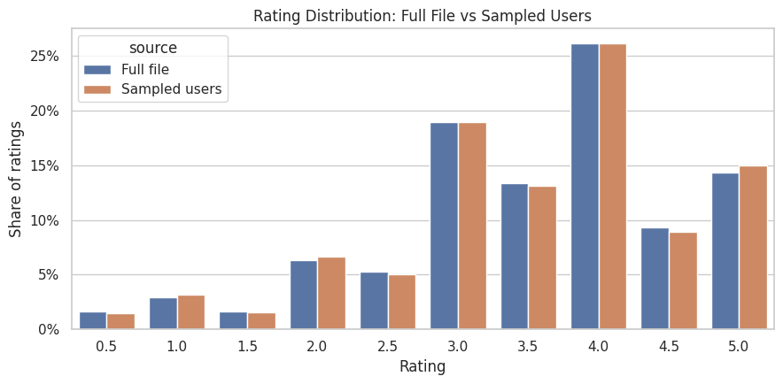
7. Plot the Rating Distribution

The table above is precise, but the plot makes the rating scale easier to read. We show full-file and sampled-user shares side by side. The liked outcome used later is based on ratings of 4.0 or higher, so the mass around 4.0 and 5.0 is especially important.

rating_plot_df = rating_distribution.melt(
    id_vars="rating",
    value_vars=["full_share", "sample_share"],
    var_name="source",
    value_name="share",
)
rating_plot_df["source"] = rating_plot_df["source"].map(
    {"full_share": "Full file", "sample_share": "Sampled users"}
)

fig, ax = plt.subplots(figsize=(9, 4.5))
sns.barplot(data=rating_plot_df, x="rating", y="share", hue="source", ax=ax)
ax.set_title("Rating Distribution: Full File vs Sampled Users")
ax.set_xlabel("Rating")
ax.set_ylabel("Share of ratings")
ax.yaxis.set_major_formatter(lambda x, _: f"{x:.0%}")
plt.tight_layout()
fig.savefig(FIGURE_DIR / "01_rating_distribution.png", dpi=160, bbox_inches="tight")
plt.show()

The sampled-user distribution should track the full distribution closely. This makes the sampled ratings acceptable for EDA, user-history features, and initial slate construction. The concentration of positive ratings also reminds us that MovieLens ratings are explicit preference events, not random impressions.

8. Join Ratings to Movie Metadata

For interference analysis, ratings alone are not enough. We need item context so we can ask whether promoted movies displace similar movies. This cell joins the sampled ratings to movie metadata and checks whether any sampled ratings lack catalog information.

ratings_enriched = ratings_sample.merge(
    movies[
        [
            "movieId",
            "title",
            "clean_title",
            "genres",
            "primary_genre",
            "genre_count",
            "release_year",
        ]
    ],
    on="movieId",
    how="left",
)

join_quality = pd.DataFrame(
    {
        "metric": [
            "sample_rating_rows",
            "rows_missing_movie_title",
            "rows_missing_primary_genre",
            "distinct_primary_genres_in_ratings",
        ],
        "value": [
            len(ratings_enriched),
            int(ratings_enriched["title"].isna().sum()),
            int(ratings_enriched["primary_genre"].isna().sum()),
            ratings_enriched["primary_genre"].nunique(),
        ],
    }
)

display(join_quality)
display(ratings_enriched.head())
metric value
0 sample_rating_rows 617851
1 rows_missing_movie_title 0
2 rows_missing_primary_genre 0
3 distinct_primary_genres_in_ratings 20
userId movieId rating timestamp rating_datetime rating_year liked title clean_title genres primary_genre genre_count release_year
0 50 32 5.0000 1262076877 2009-12-29 08:54:37 2009 1 Twelve Monkeys (a.k.a. 12 Monkeys) (1995) Twelve Monkeys (a.k.a. 12 Monkeys) Mystery|Sci-Fi|Thriller Mystery 3 1,995.0000
1 50 47 5.0000 1262077899 2009-12-29 09:11:39 2009 1 Seven (a.k.a. Se7en) (1995) Seven (a.k.a. Se7en) Mystery|Thriller Mystery 2 1,995.0000
2 50 50 5.0000 1262076691 2009-12-29 08:51:31 2009 1 Usual Suspects, The (1995) Usual Suspects, The Crime|Mystery|Thriller Crime 3 1,995.0000
3 50 163 3.5000 1262076468 2009-12-29 08:47:48 2009 0 Desperado (1995) Desperado Action|Romance|Western Action 3 1,995.0000
4 50 172 4.0000 1262076505 2009-12-29 08:48:25 2009 1 Johnny Mnemonic (1995) Johnny Mnemonic Action|Sci-Fi|Thriller Action 3 1,995.0000

The join quality check tells us whether MovieLens identifiers are internally consistent. A clean join means later notebooks can safely use movie genres, release years, and titles when defining substitute groups and explaining spillover mechanisms.

9. User Activity Distribution

Interference simulation needs users with enough history to form realistic candidate slates. This cell summarizes how many ratings each sampled user has, their average rating, their share of high ratings, and the time span of their activity.

user_features = (
    ratings_enriched.groupby("userId")
    .agg(
        n_ratings=("rating", "size"),
        mean_rating=("rating", "mean"),
        liked_rate=("liked", "mean"),
        first_rating_time=("rating_datetime", "min"),
        last_rating_time=("rating_datetime", "max"),
        active_years=("rating_year", "nunique"),
        unique_primary_genres=("primary_genre", "nunique"),
    )
    .reset_index()
)
user_features["activity_span_days"] = (
    user_features["last_rating_time"] - user_features["first_rating_time"]
).dt.days

user_activity_summary = user_features[
    ["n_ratings", "mean_rating", "liked_rate", "active_years", "activity_span_days", "unique_primary_genres"]
].describe(percentiles=[0.1, 0.25, 0.5, 0.75, 0.9]).T

display(user_activity_summary)
display(user_features.sort_values("n_ratings", ascending=False).head(10))
count mean std min 10% 25% 50% 75% 90% max
n_ratings 4,018.0000 153.7708 266.3372 20.0000 24.0000 36.0000 70.0000 162.0000 339.0000 5,160.0000
mean_rating 4,018.0000 3.7075 0.4844 0.5500 3.1160 3.4134 3.7188 4.0156 4.3028 5.0000
liked_rate 4,018.0000 0.5780 0.2041 0.0000 0.3018 0.4366 0.5815 0.7257 0.8462 1.0000
active_years 4,018.0000 1.5271 1.6525 1.0000 1.0000 1.0000 1.0000 1.0000 2.0000 20.0000
activity_span_days 4,018.0000 257.6847 809.0312 0.0000 0.0000 0.0000 0.0000 53.0000 701.3000 8,396.0000
unique_primary_genres 4,018.0000 9.2086 3.0216 2.0000 6.0000 7.0000 9.0000 11.0000 14.0000 19.0000
userId n_ratings mean_rating liked_rate first_rating_time last_rating_time active_years unique_primary_genres activity_span_days
1659 83000 5160 2.4058 0.0698 2002-08-19 19:48:36 2002-11-25 17:50:15 1 18 97
1640 82050 4681 3.3622 0.5954 2016-05-11 19:53:45 2023-10-06 02:48:47 8 19 2703
3185 159300 3714 3.0128 0.2130 2015-06-20 00:36:28 2023-10-10 00:38:25 9 19 3034
268 13450 3212 3.2425 0.2313 2015-04-28 21:23:47 2015-10-17 12:16:39 1 19 171
1059 53000 2937 3.8413 0.5788 2014-12-18 23:45:37 2021-10-23 00:32:59 5 19 2500
1334 66750 2740 3.6943 0.5544 2005-09-05 19:46:49 2023-06-24 03:41:52 10 19 6500
185 9300 2587 3.3761 0.3545 2005-08-28 08:22:39 2023-09-11 15:50:15 18 18 6588
2126 106350 2378 3.8425 0.6514 2001-06-20 21:31:57 2023-02-18 21:12:27 15 18 7912
1810 90550 2357 3.4913 0.3818 2000-04-06 22:40:10 2021-10-27 23:42:19 17 17 7874
1030 51550 2288 3.0590 0.4274 2016-03-13 17:39:09 2023-10-06 18:14:38 7 18 2763

The user activity distribution tells us how many users can support slate construction. Users with very few ratings are less useful because we cannot build a credible set of competing candidate items for them. Users with broader genre histories are especially useful because they create slates with both substitutes and non-substitutes.

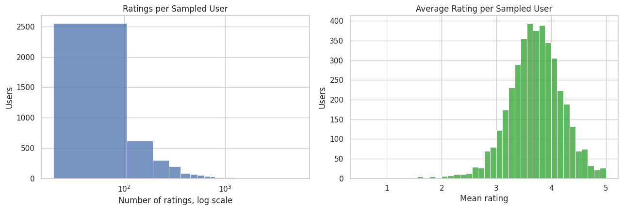
10. Plot User Activity and Rating Tendencies

This cell visualizes user heterogeneity. The left plot shows the long-tailed number of ratings per sampled user. The right plot shows the distribution of each user’s average rating. Both matter because recommendation simulations should account for heavy users and naturally generous or strict raters.

fig, axes = plt.subplots(1, 2, figsize=(13, 4.5))

sns.histplot(user_features["n_ratings"], bins=60, ax=axes[0])
axes[0].set_xscale("log")
axes[0].set_title("Ratings per Sampled User")
axes[0].set_xlabel("Number of ratings, log scale")
axes[0].set_ylabel("Users")

sns.histplot(user_features["mean_rating"], bins=40, ax=axes[1], color="tab:green")
axes[1].set_title("Average Rating per Sampled User")
axes[1].set_xlabel("Mean rating")
axes[1].set_ylabel("Users")

plt.tight_layout()
fig.savefig(FIGURE_DIR / "02_user_activity.png", dpi=160, bbox_inches="tight")
plt.show()

The log scale is intentional because user activity is usually very skewed. That skew matters for interference: a small number of very active users may create many plausible slates, while less active users may only support a few. Later simulations should avoid letting the heaviest users dominate all estimates.

11. Item Popularity and Quality Signals

This cell creates item-level features from the sampled ratings. These features describe how often each movie appears, its average rating, and its high-rating rate. Popularity is important for simulated ranking because promoted items are rarely assigned from a uniform catalog; recommendation systems tend to draw from relevant and popular candidates.

item_features = (
    ratings_enriched.groupby("movieId")
    .agg(
        sample_rating_count=("rating", "size"),
        sample_mean_rating=("rating", "mean"),
        sample_liked_rate=("liked", "mean"),
        first_sample_rating_time=("rating_datetime", "min"),
        last_sample_rating_time=("rating_datetime", "max"),
    )
    .reset_index()
    .merge(movies, on="movieId", how="left")
)

item_features["popularity_bucket"] = pd.qcut(
    item_features["sample_rating_count"].rank(method="first"),
    q=5,
    labels=["very_low", "low", "medium", "high", "very_high"],
)

top_items = item_features.sort_values("sample_rating_count", ascending=False).head(15)[
    ["movieId", "title", "primary_genre", "sample_rating_count", "sample_mean_rating", "sample_liked_rate"]
]

item_summary = item_features[
    ["sample_rating_count", "sample_mean_rating", "sample_liked_rate", "genre_count"]
].describe(percentiles=[0.1, 0.25, 0.5, 0.75, 0.9]).T

display(item_summary)
display(top_items)
count mean std min 10% 25% 50% 75% 90% max
sample_rating_count 22,313.0000 27.6902 95.9410 1.0000 1.0000 1.0000 2.0000 12.0000 56.0000 2,031.0000
sample_mean_rating 22,313.0000 3.2312 0.9839 0.5000 2.0000 2.7867 3.4000 3.8571 4.2500 5.0000
sample_liked_rate 22,313.0000 0.3893 0.3626 0.0000 0.0000 0.0000 0.3333 0.6410 1.0000 1.0000
genre_count 22,313.0000 2.0419 1.0570 1.0000 1.0000 1.0000 2.0000 3.0000 3.0000 10.0000
movieId title primary_genre sample_rating_count sample_mean_rating sample_liked_rate
306 318 Shawshank Redemption, The (1994) Crime 2031 4.4094 0.8612
285 296 Pulp Fiction (1994) Comedy 1965 4.1883 0.7913
343 356 Forrest Gump (1994) Comedy 1952 4.0666 0.7208
2371 2571 Matrix, The (1999) Action 1865 4.1550 0.7609
573 593 Silence of the Lambs, The (1991) Crime 1792 4.1083 0.7695
250 260 Star Wars: Episode IV - A New Hope (1977) Action 1710 4.0854 0.7386
2746 2959 Fight Club (1999) Action 1538 4.2048 0.7874
1103 1196 Star Wars: Episode V - The Empire Strikes Back... Action 1446 4.0992 0.7510
464 480 Jurassic Park (1993) Action 1443 3.7290 0.5703
511 527 Schindler's List (1993) Drama 1430 4.2374 0.8070
4687 4993 Lord of the Rings: The Fellowship of the Ring,... Adventure 1429 4.0896 0.7460
106 110 Braveheart (1995) Action 1390 3.9946 0.7022
48 50 Usual Suspects, The (1995) Crime 1384 4.2518 0.8071
569 589 Terminator 2: Judgment Day (1991) Action 1353 3.9327 0.6556
795 858 Godfather, The (1972) Crime 1353 4.3038 0.8130

The top movies are not just descriptive; they reveal the attention distribution that a simulated recommender would inherit. If we promote already-popular movies, displacement may mostly affect other popular substitutes. If we promote niche movies, spillovers may look different. This is why popularity buckets are saved as item features.

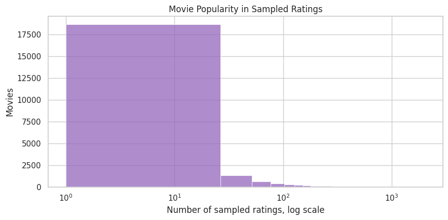
12. Plot the Item Popularity Long Tail

Recommendation catalogs usually have a long tail: a few items receive many interactions, while most items receive few. This plot checks whether the MovieLens sample has that shape. A long tail is useful here because spillovers can be studied across popular, medium, and niche items.

fig, ax = plt.subplots(figsize=(9, 4.5))
sns.histplot(item_features["sample_rating_count"], bins=80, ax=ax, color="tab:purple")
ax.set_xscale("log")
ax.set_title("Movie Popularity in Sampled Ratings")
ax.set_xlabel("Number of sampled ratings, log scale")
ax.set_ylabel("Movies")
plt.tight_layout()
fig.savefig(FIGURE_DIR / "03_item_popularity_long_tail.png", dpi=160, bbox_inches="tight")
plt.show()

The long-tail pattern supports the simulation plan. Interference is partly about scarce attention, and scarce attention is most interesting when items vary widely in baseline popularity. This also gives later notebooks a reason to report effects separately by item popularity tier.

13. Genre Coverage and Substitute Groups

Genres are the first approximation to item clusters. This cell explodes the multi-genre movie table so each movie contributes to every genre it belongs to, then computes catalog size, rating volume, average rating, and liked rate by genre.

movie_genres = movies[["movieId", "genre_list"]].explode("genre_list").rename(columns={"genre_list": "genre"})

rating_genres = ratings_sample[["movieId", "rating", "liked"]].merge(movie_genres, on="movieId", how="left")

genre_summary = (
    rating_genres.groupby("genre")
    .agg(
        sampled_rating_rows=("rating", "size"),
        unique_movies=("movieId", "nunique"),
        mean_rating=("rating", "mean"),
        liked_rate=("liked", "mean"),
    )
    .reset_index()
    .sort_values("sampled_rating_rows", ascending=False)
)

display(genre_summary)
genre sampled_rating_rows unique_movies mean_rating liked_rate
8 Drama 271190 9867 3.6791 0.5567
5 Comedy 215975 7010 3.4352 0.4565
1 Action 186192 3443 3.4850 0.4668
17 Thriller 167555 4070 3.5485 0.4938
2 Adventure 145711 2042 3.5298 0.4885
16 Sci-Fi 111123 1878 3.5124 0.4816
15 Romance 107165 3354 3.5506 0.5035
6 Crime 104853 2332 3.6946 0.5596
9 Fantasy 70853 1422 3.5189 0.4870
4 Children 51351 1239 3.4301 0.4579
14 Mystery 50611 1233 3.6846 0.5569
11 Horror 46883 2395 3.3446 0.4185
3 Animation 41736 1247 3.6112 0.5270
18 War 31009 814 3.7865 0.6047
12 IMAX 28710 175 3.5887 0.5039
13 Musical 21602 526 3.5132 0.4911
19 Western 11645 393 3.5910 0.5198
7 Documentary 8024 1516 3.6344 0.5581
10 Film-Noir 6138 174 3.9195 0.6795
0 (no genres listed) 953 431 3.4418 0.4953

The genre summary gives the first map of possible spillover neighborhoods. Large genres such as drama or comedy can support many within-genre substitute comparisons. Smaller genres may need to be combined or treated cautiously because sparse clusters can create noisy spillover estimates.

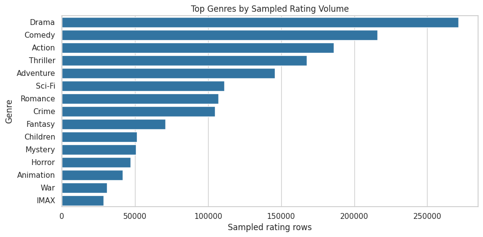
14. Plot Rating Volume by Genre

This visualization highlights which genres dominate the sampled preference data. For interference modeling, this helps decide where simulated slates will have enough similar items to create meaningful within-cluster competition.

top_genres = genre_summary.head(15).copy()

fig, ax = plt.subplots(figsize=(10, 5))
sns.barplot(data=top_genres, x="sampled_rating_rows", y="genre", ax=ax, color="tab:blue")
ax.set_title("Top Genres by Sampled Rating Volume")
ax.set_xlabel("Sampled rating rows")
ax.set_ylabel("Genre")
plt.tight_layout()
fig.savefig(FIGURE_DIR / "04_genre_rating_volume.png", dpi=160, bbox_inches="tight")
plt.show()

The largest genres are natural starting points for substitute clusters. Later, when we simulate a promoted item, we can define spillover exposure as the number or share of same-genre items promoted nearby in the same slate. That turns genre EDA into a causal exposure model.

15. Time Coverage in the Rating Sample

MovieLens spans many years. This cell summarizes rating volume over calendar time so we can see whether the sample covers the same broad period as the full file. Time matters because user preferences, catalog composition, and platform behavior can all drift.

yearly_activity = (
    ratings_sample.groupby("rating_year")
    .agg(
        rating_rows=("rating", "size"),
        users=("userId", "nunique"),
        movies=("movieId", "nunique"),
        mean_rating=("rating", "mean"),
        liked_rate=("liked", "mean"),
    )
    .reset_index()
)

display(yearly_activity.head())
display(yearly_activity.tail())
rating_year rating_rows users movies mean_rating liked_rate
0 1996 31909 510 1030 3.5553 0.4914
1 1997 12671 225 1161 3.5889 0.5097
2 1998 6167 82 1396 3.6142 0.5821
3 1999 21873 197 2177 3.6783 0.6207
4 2000 40933 299 3095 3.5898 0.5754
rating_year rating_rows users movies mean_rating liked_rate
23 2019 28206 247 5998 3.6410 0.5284
24 2020 31039 265 7148 3.5423 0.4982
25 2021 22974 241 5981 3.6466 0.5339
26 2022 18050 215 5139 3.7061 0.5532
27 2023 20494 186 5242 3.6596 0.5222

The yearly table checks temporal breadth and gives a first look at drift. We do not need to solve time drift in the first notebook, but later simulations should avoid accidentally mixing very old and very recent behavior without acknowledging it.

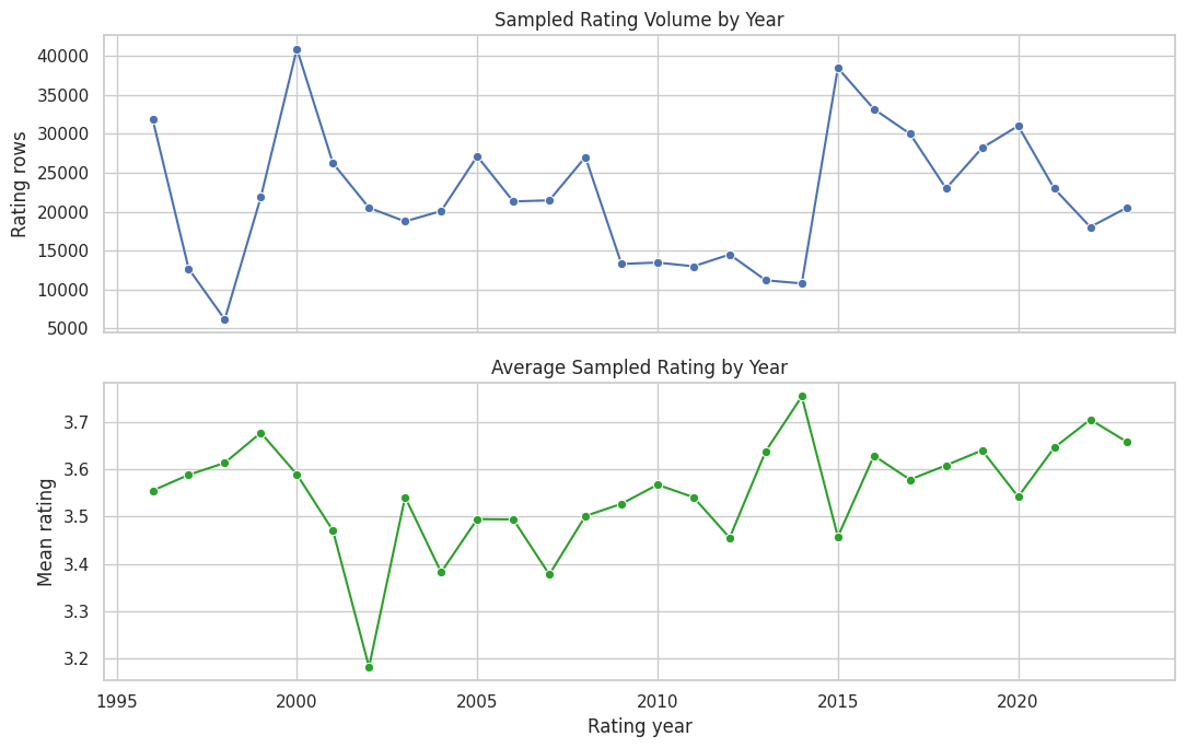
16. Plot Yearly Rating Activity

The plot makes the time trend easier to see than the table. We show sampled rating volume and average rating by year. This helps identify whether a small number of years dominate the sample.

fig, axes = plt.subplots(2, 1, figsize=(11, 7), sharex=True)

sns.lineplot(data=yearly_activity, x="rating_year", y="rating_rows", marker="o", ax=axes[0])
axes[0].set_title("Sampled Rating Volume by Year")
axes[0].set_ylabel("Rating rows")
axes[0].set_xlabel("")

sns.lineplot(data=yearly_activity, x="rating_year", y="mean_rating", marker="o", ax=axes[1], color="tab:green")
axes[1].set_title("Average Sampled Rating by Year")
axes[1].set_ylabel("Mean rating")
axes[1].set_xlabel("Rating year")

plt.tight_layout()
fig.savefig(FIGURE_DIR / "05_yearly_rating_activity.png", dpi=160, bbox_inches="tight")
plt.show()

The time trend is useful for deciding whether future notebooks should include calendar controls. Even in a simulation project, realistic time structure matters because old and new catalog items may have different popularity and competition patterns.

17. Top Tags in the Sample

This cell inspects the most common cleaned tags. Tags often capture actors, franchises, moods, themes, and other semantics that genres miss. We will not use them as the first cluster definition, but seeing them helps explain how the project could be extended beyond genre-level spillovers.

top_tags = (
    tags_sample.dropna(subset=["tag_clean"])
    .groupby("tag_clean")
    .agg(tag_rows=("tag_clean", "size"), users=("userId", "nunique"), movies=("movieId", "nunique"))
    .reset_index()
    .sort_values("tag_rows", ascending=False)
    .head(25)
)

display(top_tags)
tag_clean tag_rows users movies
22173 sci-fi 2562 667 474
2051 atmospheric 2418 503 536
609 action 2354 461 686
5411 comedy 2204 503 887
9942 funny 2075 489 774
27109 visually appealing 1628 482 295
24606 surreal 1596 488 345
21607 romance 1469 351 654
26232 twist ending 1459 482 224
25439 thought-provoking 1391 469 245
6364 dark comedy 1282 436 243
7700 dystopia 1206 370 196
20504 quirky 1181 343 319
23404 social commentary 1181 339 325
24368 stylized 1177 287 360
5011 cinematography 1173 347 342
2633 based on a book 1115 279 487
757 adventure 1109 320 322
6360 dark 1085 354 268
25459 thriller 1064 326 363
20339 psychology 1050 385 161
11923 horror 1044 276 384
8900 fantasy 1029 331 312
3536 boring 1004 267 704
5084 classic 1000 358 286

The tag sample suggests richer semantic neighborhoods are possible. For example, two movies in different genres might still compete if they share an actor, franchise, mood, or theme. The first version of the project will stay with genres for clarity, but tags are a credible future refinement.

18. Define an Interference-Ready Item Table

This cell creates the item table that later notebooks can reuse. It combines catalog metadata with sampled popularity and preference features. It also defines spillover_cluster, a first-pass substitute group based on primary genre. This is intentionally simple and explainable.

interference_items = item_features.assign(
    spillover_cluster=item_features["primary_genre"].fillna("unknown"),
    is_broad_release_year=item_features["release_year"].notna().astype("int8"),
)[
    [
        "movieId",
        "title",
        "clean_title",
        "genres",
        "primary_genre",
        "spillover_cluster",
        "release_year",
        "genre_count",
        "sample_rating_count",
        "sample_mean_rating",
        "sample_liked_rate",
        "popularity_bucket",
    ]
].copy()

cluster_readiness = (
    interference_items.groupby("spillover_cluster")
    .agg(
        movies=("movieId", "nunique"),
        sampled_ratings=("sample_rating_count", "sum"),
        mean_item_rating=("sample_mean_rating", "mean"),
    )
    .reset_index()
    .sort_values("sampled_ratings", ascending=False)
)

display(cluster_readiness.head(20))
spillover_cluster movies sampled_ratings mean_item_rating
1 Action 3443 186192 3.1305
5 Comedy 5432 139545 3.1890
8 Drama 5580 116649 3.3018
2 Adventure 1116 61465 3.1763
6 Crime 1196 44116 3.4327
11 Horror 1306 16833 2.8955
3 Animation 706 14465 3.2919
4 Children 427 10747 3.1775
7 Documentary 1372 6739 3.3269
14 Mystery 124 6230 3.4562
17 Thriller 331 4520 3.2861
16 Sci-Fi 227 3232 3.0557
9 Fantasy 140 2264 3.0980
19 Western 114 1240 3.4242
15 Romance 272 991 4.3652
0 (no genres listed) 431 953 3.1554
10 Film-Noir 23 815 3.5313
13 Musical 43 720 3.0830
18 War 29 134 3.3824
12 IMAX 1 1 3.0000

The spillover_cluster column is the bridge from EDA to causal design. In later notebooks, a movie’s potential outcomes can depend on its own promotion and on the promotion intensity among other movies in the same cluster or slate.

19. Build a Seed Dataset for Simulated Slates

MovieLens does not tell us which movies were shown together, so later notebooks need to simulate slates. This cell creates a seed table by selecting active users and taking a bounded set of their recent, highly rated movies. Each user’s seed slate is not yet a randomized experiment; it is a realistic candidate set that later notebooks can rank, promote, and use for spillover exposure construction.

MIN_USER_RATINGS_FOR_SLATE = 20
SLATE_SIZE = 12
MAX_SEED_USERS = 3_000
RECENT_POOL_SIZE = 50

eligible_users = (
    user_features.query("n_ratings >= @MIN_USER_RATINGS_FOR_SLATE")
    .sort_values(["n_ratings", "unique_primary_genres"], ascending=False)
    .head(MAX_SEED_USERS)["userId"]
)

recent_pool = (
    ratings_enriched.loc[ratings_enriched["userId"].isin(eligible_users)]
    .sort_values(["userId", "rating_datetime"], ascending=[True, False])
    .assign(recent_rank=lambda df: df.groupby("userId").cumcount() + 1)
    .query("recent_rank <= @RECENT_POOL_SIZE")
)

slate_seed = (
    recent_pool.sort_values(["userId", "rating", "rating_datetime"], ascending=[True, False, False])
    .groupby("userId", group_keys=False)
    .head(SLATE_SIZE)
    .copy()
)

slate_seed["slate_id"] = "user_" + slate_seed["userId"].astype(str) + "_seed"
slate_seed["slate_position_seed"] = slate_seed.groupby("userId").cumcount() + 1
slate_seed["observed_relevance"] = slate_seed["rating"]
slate_seed["high_relevance"] = (slate_seed["rating"] >= 4.0).astype("int8")
slate_seed["spillover_cluster"] = slate_seed["primary_genre"].fillna("unknown")

complete_slate_ids = (
    slate_seed.groupby("slate_id").size().loc[lambda size: size == SLATE_SIZE].index
)
slate_seed = slate_seed.loc[slate_seed["slate_id"].isin(complete_slate_ids)].copy()

slate_seed = slate_seed[
    [
        "slate_id",
        "userId",
        "movieId",
        "title",
        "genres",
        "primary_genre",
        "spillover_cluster",
        "slate_position_seed",
        "observed_relevance",
        "high_relevance",
        "rating_datetime",
        "rating_year",
    ]
]

slate_seed_summary = pd.DataFrame(
    {
        "metric": [
            "eligible_users_considered",
            "complete_seed_slates",
            "rows_in_seed_slate_table",
            "slate_size",
            "unique_movies_in_seed_slates",
            "unique_spillover_clusters",
            "mean_high_relevance_rate",
        ],
        "value": [
            len(eligible_users),
            slate_seed["slate_id"].nunique(),
            len(slate_seed),
            SLATE_SIZE,
            slate_seed["movieId"].nunique(),
            slate_seed["spillover_cluster"].nunique(),
            slate_seed["high_relevance"].mean(),
        ],
    }
)

display(slate_seed_summary)
display(slate_seed.head(15))
metric value
0 eligible_users_considered 3,000.0000
1 complete_seed_slates 3,000.0000
2 rows_in_seed_slate_table 36,000.0000
3 slate_size 12.0000
4 unique_movies_in_seed_slates 5,668.0000
5 unique_spillover_clusters 19.0000
6 mean_high_relevance_rate 0.9596
slate_id userId movieId title genres primary_genre spillover_cluster slate_position_seed observed_relevance high_relevance rating_datetime rating_year
74 user_50_seed 50 4027 O Brother, Where Art Thou? (2000) Adventure|Comedy|Crime Adventure Adventure 1 5.0000 1 2009-12-31 06:58:12 2009
27 user_50_seed 50 1196 Star Wars: Episode V - The Empire Strikes Back... Action|Adventure|Sci-Fi Action Action 2 5.0000 1 2009-12-29 09:12:16 2009
1 user_50_seed 50 47 Seven (a.k.a. Se7en) (1995) Mystery|Thriller Mystery Mystery 3 5.0000 1 2009-12-29 09:11:39 2009
101 user_50_seed 50 52435 How the Grinch Stole Christmas! (1966) Animation|Comedy|Fantasy|Musical Animation Animation 4 5.0000 1 2009-12-29 09:10:49 2009
36 user_50_seed 50 1214 Alien (1979) Horror|Sci-Fi Horror Horror 5 5.0000 1 2009-12-29 09:09:28 2009
49 user_50_seed 50 1288 This Is Spinal Tap (1984) Comedy Comedy Comedy 6 5.0000 1 2009-12-29 09:09:18 2009
11 user_50_seed 50 593 Silence of the Lambs, The (1991) Crime|Horror|Thriller Crime Crime 7 5.0000 1 2009-12-29 09:08:00 2009
25 user_50_seed 50 1136 Monty Python and the Holy Grail (1975) Adventure|Comedy|Fantasy Adventure Adventure 8 5.0000 1 2009-12-29 09:05:51 2009
67 user_50_seed 50 2959 Fight Club (1999) Action|Crime|Drama|Thriller Action Action 9 5.0000 1 2009-12-29 09:05:21 2009
52 user_50_seed 50 1617 L.A. Confidential (1997) Crime|Film-Noir|Mystery|Thriller Crime Crime 10 5.0000 1 2009-12-29 09:04:30 2009
12 user_50_seed 50 608 Fargo (1996) Comedy|Crime|Drama|Thriller Comedy Comedy 11 5.0000 1 2009-12-29 09:04:23 2009
47 user_50_seed 50 1276 Cool Hand Luke (1967) Drama Drama Drama 12 4.5000 1 2009-12-29 09:14:25 2009
279 user_100_seed 100 55820 No Country for Old Men (2007) Crime|Drama Crime Crime 1 5.0000 1 2021-05-04 09:20:43 2021
269 user_100_seed 100 48394 Pan's Labyrinth (Laberinto del fauno, El) (2006) Drama|Fantasy|Thriller Drama Drama 2 5.0000 1 2021-05-04 09:20:40 2021
325 user_100_seed 100 99114 Django Unchained (2012) Action|Drama|Western Action Action 3 5.0000 1 2021-05-04 09:19:58 2021

The seed slate table is the key handoff from this notebook. It gives later notebooks user-specific candidate sets with item metadata and relevance labels. The next notebook can now focus on exposure mapping: which items are promoted, which same-cluster items are spillover-exposed, and how promotion changes simulated slate outcomes.

20. Save Processed Inputs

This cell saves the cleaned sample tables and readiness summaries. Saving these files keeps later notebooks fast and consistent: they can load the same sampled users, item features, and seed slates instead of repeating the expensive zip scan.

ratings_output = PROCESSED_DIR / "movielens_interference_ratings_sample.parquet"
items_output = PROCESSED_DIR / "movielens_interference_items.parquet"
users_output = PROCESSED_DIR / "movielens_interference_user_features.parquet"
slates_output = PROCESSED_DIR / "movielens_interference_slate_seed.parquet"
readiness_output = PROCESSED_DIR / "movielens_interference_setup_readiness.csv"

ratings_enriched.to_parquet(ratings_output, index=False)
interference_items.to_parquet(items_output, index=False)
user_features.to_parquet(users_output, index=False)
slate_seed.to_parquet(slates_output, index=False)

readiness_checks = pd.DataFrame(
    [
        {
            "check": "raw_zip_found",
            "value": bool(RAW_ZIP.exists()),
            "notes": "MovieLens zip file is available locally.",
        },
        {
            "check": "ratings_sample_rows",
            "value": len(ratings_enriched),
            "notes": "Sample contains complete histories for selected users.",
        },
        {
            "check": "sample_unique_users",
            "value": ratings_enriched["userId"].nunique(),
            "notes": "Users available for user-level slate simulation.",
        },
        {
            "check": "sample_unique_movies",
            "value": ratings_enriched["movieId"].nunique(),
            "notes": "Movies available for item-level spillover analysis.",
        },
        {
            "check": "complete_seed_slates",
            "value": slate_seed["slate_id"].nunique(),
            "notes": "Complete seed slates available for exposure simulation.",
        },
        {
            "check": "seed_slate_rows",
            "value": len(slate_seed),
            "notes": "Rows in the slate seed table; should equal complete slates times slate size.",
        },
        {
            "check": "spillover_clusters",
            "value": interference_items["spillover_cluster"].nunique(),
            "notes": "Initial substitute clusters based on primary genre.",
        },
    ]
)
readiness_checks.to_csv(readiness_output, index=False)

saved_files = pd.DataFrame(
    {
        "artifact": [
            "ratings_sample",
            "interference_items",
            "user_features",
            "slate_seed",
            "readiness_checks",
        ],
        "path": [
            str(ratings_output),
            str(items_output),
            str(users_output),
            str(slates_output),
            str(readiness_output),
        ],
    }
)

display(readiness_checks)
display(saved_files)
check value notes
0 raw_zip_found True MovieLens zip file is available locally.
1 ratings_sample_rows 617851 Sample contains complete histories for selecte...
2 sample_unique_users 4018 Users available for user-level slate simulation.
3 sample_unique_movies 22313 Movies available for item-level spillover anal...
4 complete_seed_slates 3000 Complete seed slates available for exposure si...
5 seed_slate_rows 36000 Rows in the slate seed table; should equal com...
6 spillover_clusters 20 Initial substitute clusters based on primary g...
artifact path
0 ratings_sample /home/apex/Documents/ranking_sys/data/processe...
1 interference_items /home/apex/Documents/ranking_sys/data/processe...
2 user_features /home/apex/Documents/ranking_sys/data/processe...
3 slate_seed /home/apex/Documents/ranking_sys/data/processe...
4 readiness_checks /home/apex/Documents/ranking_sys/data/processe...

The processed files make the interference project reproducible and modular. The important output is the seed slate table because it gives the next notebook a realistic starting point for simulating promotion assignments and spillover exposure. The user and item feature tables provide adjustment and segmentation variables.

21. Notebook Takeaways

This notebook established the foundation for an interference/spillover analysis using MovieLens:

  • MovieLens has strong user-item preference data but no true impression logs, so the causal design must be simulated.
  • Ratings provide a preference/relevance signal, while genres provide a transparent first substitute-cluster definition.
  • The sampled-user strategy keeps complete histories for selected users, which is more useful than isolated row sampling.
  • The seed slate table creates realistic user-specific candidate sets for later promotion and spillover simulations.
  • The next notebook should define exposure mappings: direct promotion, same-slate spillover exposure, same-cluster spillover exposure, and slate-level outcome construction.