07 Final Report And Artifacts

This notebook packages Off-Policy Evaluation of Recommendation Systems into portfolio-ready outputs.

The earlier notebooks did the technical work:

• Notebook 1: Open Bandit EDA
• Notebook 2: behavior policy and propensity diagnostics
• Notebook 3: IPS and SNIPS
• Notebook 4: doubly robust OPE
• Notebook 5: policy comparison and sensitivity
• Notebook 6: contextual policy learning

This final notebook does not introduce a new estimator. Its job is to turn the completed analysis into clean tables, figures, final recommendations, limitations, and resume-ready writing.

Final Notebook Goal

A portfolio project should end with an artifact that a hiring manager or interviewer can understand quickly.

This notebook answers:

• What problem did the project solve?
• Which dataset and causal setup were used?
• Which estimators were implemented?
• Which recommendation policy is the best offline candidate for online testing?
• How stable is that recommendation?
• What limitations remain?

The final recommendation is intentionally cautious. Offline OPE can prioritize a policy for A/B testing, but it cannot prove production lift by itself.

Notebook Setup

This cell imports plotting and data libraries, sets display options, and defines a small helper for saving figures.

The notebook reads already-generated tables from notebooks/projects/project_2_off_policy_evaluation/writeup/tables/. That keeps the final report fast and reproducible without retraining models.

from pathlib import Path

import matplotlib.pyplot as plt
import numpy as np
import pandas as pd
import seaborn as sns

pd.set_option("display.max_columns", 140)
pd.set_option("display.max_rows", 140)
pd.set_option("display.float_format", "{:.6f}".format)

sns.set_theme(style="whitegrid", context="notebook")

This cell prepares the notebook environment for final OPE report and portfolio artifacts. There is no estimator output yet; the main value is that the imports, display settings, and plotting defaults are ready for the OPE diagnostics that follow.

Locate Project And Writeup Folders

This cell finds the repository root and creates the final writeup folders.

All final off-policy evaluation artifacts are written inside notebooks/projects/project_2_off_policy_evaluation/writeup/ so they stay colocated with the notebooks. Figures go into figures/, tables go into tables/, and markdown snippets go into the writeup root.

TABLE_RELATIVE_PATH = Path("notebooks/projects/project_2_off_policy_evaluation/writeup/tables/main_lgbm_ope_estimates.csv")
PROJECT_ROOT = next(
    path
    for path in [Path.cwd(), *Path.cwd().parents]
    if (path / TABLE_RELATIVE_PATH).exists()
)

WRITEUP_DIR = PROJECT_ROOT / "notebooks/projects/project_2_off_policy_evaluation/writeup"
FIGURE_DIR = WRITEUP_DIR / "figures"
TABLE_DIR = WRITEUP_DIR / "tables"

FIGURE_DIR.mkdir(parents=True, exist_ok=True)
TABLE_DIR.mkdir(parents=True, exist_ok=True)

pd.Series(
    {
        "project_root": PROJECT_ROOT,
        "writeup_dir": WRITEUP_DIR,
        "figure_dir": FIGURE_DIR,
        "table_dir": TABLE_DIR,
    }
).to_frame("value")

	value
project_root	/home/apex/Documents/ranking_sys
writeup_dir	/home/apex/Documents/ranking_sys/notebooks/off...
figure_dir	/home/apex/Documents/ranking_sys/notebooks/off...
table_dir	/home/apex/Documents/ranking_sys/notebooks/off...

The printed paths are a reproducibility checkpoint. Once the notebook can find the cached data and writeup folders, the rest of the analysis can run without manual path edits.

Load Final Analysis Tables

This cell loads the tables produced by Notebooks 5 and 6.

These tables contain the main OPE estimates, sensitivity checks, policy risk diagnostics, and contextual policy results. The final report notebook treats them as the source of truth for packaging.

def load_table(name):
    path = TABLE_DIR / name
    if not path.exists():
        raise FileNotFoundError(f"Missing required table: {path}")
    return pd.read_csv(path)

main_lgbm = load_table("main_lgbm_ope_estimates.csv")
policy_risk = load_table("policy_risk_table.csv")
clipping_stability = load_table("clipping_stability.csv")
reward_model_rank = load_table("reward_model_rank_stability.csv")
split_rank = load_table("split_rank_stability.csv")
contextual_estimates = load_table("contextual_policy_estimates.csv")
contextual_audit = load_table("contextual_policy_audit.csv")
contextual_weights = load_table("contextual_weight_diagnostics.csv")
contextual_clipping = load_table("contextual_clipping_stability.csv")
contextual_decision = load_table("contextual_policy_decision_table.csv")

loaded_tables = pd.DataFrame(
    {
        "table": [
            "main_lgbm",
            "policy_risk",
            "clipping_stability",
            "reward_model_rank",
            "split_rank",
            "contextual_estimates",
            "contextual_audit",
            "contextual_weights",
            "contextual_clipping",
            "contextual_decision",
        ],
        "rows": [
            len(main_lgbm),
            len(policy_risk),
            len(clipping_stability),
            len(reward_model_rank),
            len(split_rank),
            len(contextual_estimates),
            len(contextual_audit),
            len(contextual_weights),
            len(contextual_clipping),
            len(contextual_decision),
        ],
    }
)

loaded_tables

	table	rows
0	main_lgbm	16
1	policy_risk	4
2	clipping_stability	12
3	reward_model_rank	4
4	split_rank	4
5	contextual_estimates	24
6	contextual_audit	6
7	contextual_weights	6
8	contextual_clipping	6
9	contextual_decision	6

The loaded table shape and preview confirm that the expected cached data is available. This check matters because all later OPE estimates depend on using the correct logged actions, rewards, contexts, and behavior propensities.

Project Method Timeline

This table summarizes the technical arc of the project.

It is useful in a final report because it shows that the work moved from data validation to estimators, then to sensitivity checks and contextual policy learning. That progression matters for a portfolio: it demonstrates both causal inference fundamentals and recommendation-system judgment.

method_timeline = pd.DataFrame(
    [
        {
            "stage": "Dataset understanding",
            "notebook": "01_open_bandit_eda.ipynb",
            "purpose": "Verify actions, rewards, contexts, and logged propensities.",
        },
        {
            "stage": "Behavior-policy diagnostics",
            "notebook": "02_behavior_policy_and_propensities.ipynb",
            "purpose": "Check positivity, action support, propensity distributions, and IPS weight risk.",
        },
        {
            "stage": "Classical OPE",
            "notebook": "03_ips_and_snips.ipynb",
            "purpose": "Estimate fixed policy values with IPS and SNIPS.",
        },
        {
            "stage": "Doubly robust OPE",
            "notebook": "04_doubly_robust_ope.ipynb",
            "purpose": "Train reward models and combine direct method with residual correction.",
        },
        {
            "stage": "Sensitivity analysis",
            "notebook": "05_policy_comparison_and_sensitivity.ipynb",
            "purpose": "Stress-test conclusions across clipping, reward models, and time splits.",
        },
        {
            "stage": "Advanced contextual policy learning",
            "notebook": "06_contextual_policy_learning.ipynb",
            "purpose": "Learn context-aware policies from reward-model scores and evaluate them with DR OPE.",
        },
        {
            "stage": "Final packaging",
            "notebook": "07_final_report_and_artifacts.ipynb",
            "purpose": "Create final figures, tables, recommendations, and portfolio text.",
        },
    ]
)

method_timeline

	stage	notebook	purpose
0	Dataset understanding	01_open_bandit_eda.ipynb	Verify actions, rewards, contexts, and logged ...
1	Behavior-policy diagnostics	02_behavior_policy_and_propensities.ipynb	Check positivity, action support, propensity d...
2	Classical OPE	03_ips_and_snips.ipynb	Estimate fixed policy values with IPS and SNIPS.
3	Doubly robust OPE	04_doubly_robust_ope.ipynb	Train reward models and combine direct method ...
4	Sensitivity analysis	05_policy_comparison_and_sensitivity.ipynb	Stress-test conclusions across clipping, rewar...
5	Advanced contextual policy learning	06_contextual_policy_learning.ipynb	Learn context-aware policies from reward-model...
6	Final packaging	07_final_report_and_artifacts.ipynb	Create final figures, tables, recommendations,...

The timeline organizes the project story from raw logs to final recommendation. This helps a reviewer understand how each notebook contributes to the final OPE decision.

Final Fixed-Policy OPE Table

This table focuses on the strongest fixed-policy results from Notebook 5.

The fixed-policy recommendation is useful as a conservative baseline. These policies do not personalize by context, but they have clearer support than aggressive learned policies. The table uses LightGBM doubly robust estimates and includes sensitivity diagnostics.

fixed_policy_final = policy_risk.copy()
fixed_policy_final["policy_type"] = "fixed"
fixed_policy_final["recommendation_role"] = np.where(
    fixed_policy_final["policy"] == "ctr_weighted",
    "stable fixed-policy candidate",
    "fixed-policy benchmark",
)
fixed_policy_final = fixed_policy_final[
    [
        "policy_type",
        "policy",
        "recommendation_role",
        "estimate",
        "ci_95_lower",
        "ci_95_upper",
        "lift_pp",
        "relative_lift_pct",
        "ess_share",
        "max_weight",
        "avg_rank_across_splits",
        "dr_estimate_range_across_splits",
        "decision_score",
    ]
].sort_values("estimate", ascending=False)

fixed_policy_final

	policy_type	policy	recommendation_role	estimate	ci_95_lower	ci_95_upper	lift_pp	relative_lift_pct	ess_share	max_weight	avg_rank_across_splits	dr_estimate_range_across_splits	decision_score
3	fixed	epsilon_greedy_top_ctr	fixed-policy benchmark	0.006622	0.004035	0.009209	0.164171	32.966042	0.040290	29.050000	2.000000	0.004269	-3.658854
2	fixed	ctr_weighted	stable fixed-policy candidate	0.005282	0.004759	0.005805	0.030172	6.058681	0.790628	2.740842	1.666667	0.001205	-0.660579
0	fixed	uniform	fixed-policy benchmark	0.005034	0.004592	0.005476	0.005411	1.086540	1.000000	1.000000	3.333333	0.001374	-0.927922
1	fixed	exposure_popularity	fixed-policy benchmark	0.005020	0.004578	0.005462	0.003997	0.802658	0.996399	1.132200	3.000000	0.001285	-0.859223

The final table distills the offline evidence into a small set of decision-relevant rows. This is the version most useful for a portfolio writeup or stakeholder-facing summary.

Figure 1: Fixed-Policy Value Estimates

This figure compares IPS, SNIPS, and DR estimates for the fixed policies.

The figure is designed for the final report. DR is the preferred estimator, but IPS and SNIPS remain useful benchmarks because they show how much the answer depends on modeling assumptions.

fixed_plot = main_lgbm.query("estimator in ['IPS', 'SNIPS', 'DR']").copy()
fixed_plot["lower_error"] = fixed_plot["estimate"] - fixed_plot["ci_95_lower"]
fixed_plot["upper_error"] = fixed_plot["ci_95_upper"] - fixed_plot["estimate"]

policy_order = fixed_plot["policy"].drop_duplicates().tolist()
estimator_order = ["IPS", "SNIPS", "DR"]
offsets = {"IPS": -0.22, "SNIPS": 0.0, "DR": 0.22}
colors = {"IPS": "#F58518", "SNIPS": "#54A24B", "DR": "#B279A2"}

fig, ax = plt.subplots(figsize=(11, 5))
for estimator in estimator_order:
    subset = fixed_plot[fixed_plot["estimator"] == estimator]
    for _, row in subset.iterrows():
        x_base = policy_order.index(row["policy"])
        x = x_base + offsets[estimator]
        ax.errorbar(
            x=x,
            y=row["estimate"],
            yerr=[[row["lower_error"]], [row["upper_error"]]],
            fmt="o",
            color=colors[estimator],
            ecolor=colors[estimator],
            capsize=4,
            linewidth=1.4,
            markersize=6,
            label=estimator if row["policy"] == subset["policy"].iloc[0] else None,
        )

baseline = main_lgbm["eval_observed_click_rate"].iloc[0]
ax.axhline(baseline, color="black", linestyle="--", linewidth=1, label="Observed random")
ax.set_xticks(range(len(policy_order)))
ax.set_xticklabels(policy_order, rotation=25, ha="right")
ax.set_title("Fixed-Policy OPE Estimates")
ax.set_xlabel("Evaluation Policy")
ax.set_ylabel("Estimated Click Rate")
ax.yaxis.set_major_formatter(lambda y, _: f"{y:.2%}")
ax.legend(title="Estimator")
plt.tight_layout()

fixed_estimate_figure = FIGURE_DIR / "01_fixed_policy_ope_estimates.png"
fig.savefig(fixed_estimate_figure, dpi=180, bbox_inches="tight")
plt.show()

fixed_estimate_figure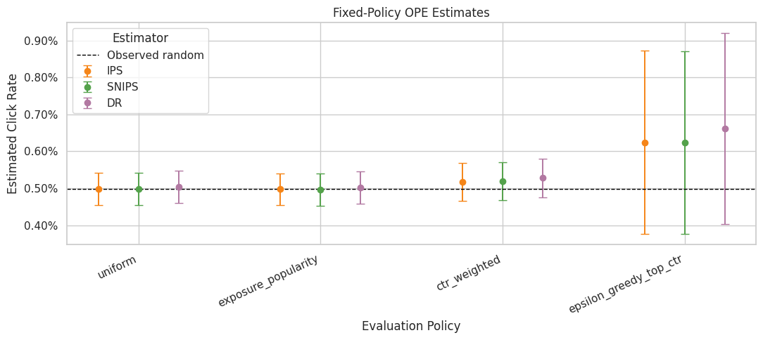

PosixPath('/home/apex/Documents/ranking_sys/notebooks/projects/project_2_off_policy_evaluation/writeup/figures/01_fixed_policy_ope_estimates.png')

The estimate plot compares policies on the same offline value scale. Error bars and estimator differences are just as important as the ranking, because high-variance estimates should not drive product decisions alone.

Final Contextual-Policy Decision Table

This table summarizes the advanced contextual policies from Notebook 6.

The important interpretation is the tradeoff between value and support. Greedy policies may have higher point estimates, but low ESS and clipping sensitivity make them risky. Conservative contextual mixtures can be more realistic candidates for online testing.

contextual_final = contextual_decision.copy()
contextual_final["policy_type"] = np.where(
    contextual_final["policy"].str.startswith("lgbm"), "contextual", "fixed benchmark"
)
contextual_final["recommendation_role"] = np.select(
    [
        contextual_final["policy"] == "lgbm_conservative_mix",
        contextual_final["policy"] == "fixed_ctr_weighted",
        contextual_final["risk_flag"].isin(["low ESS", "clip sensitive"]),
    ],
    [
        "primary contextual A/B-test candidate",
        "stable fixed-policy fallback",
        "high-value but fragile offline estimate",
    ],
    default="benchmark",
)
contextual_final = contextual_final[
    [
        "policy_type",
        "policy",
        "recommendation_role",
        "estimate",
        "ci_95_lower",
        "ci_95_upper",
        "lift_pp",
        "relative_lift_pct",
        "ess_share",
        "max_weight",
        "p99_weight",
        "dr_estimate_range",
        "support_adjusted_lift_pp",
        "risk_flag",
    ]
]

contextual_final

	policy_type	policy	recommendation_role	estimate	ci_95_lower	ci_95_upper	lift_pp	relative_lift_pct	ess_share	max_weight	p99_weight	dr_estimate_range	support_adjusted_lift_pp	risk_flag
0	contextual	lgbm_greedy	high-value but fragile offline estimate	0.007513	0.003857	0.011170	0.253344	50.872251	0.029100	34.000000	34.000000	0.027226	0.043217	low ESS
1	contextual	lgbm_epsilon_greedy	high-value but fragile offline estimate	0.007142	0.004016	0.010267	0.216160	43.405703	0.039955	29.050000	29.050000	0.022579	0.043208	low ESS
2	contextual	lgbm_softmax	high-value but fragile offline estimate	0.006001	0.003518	0.008484	0.102106	20.503156	0.168632	34.000000	5.113957	0.018609	0.041930	clip sensitive
3	contextual	lgbm_conservative_mix	primary contextual A/B-test candidate	0.005324	0.004434	0.006215	0.034450	6.917631	0.694032	10.900000	2.234187	0.003497	0.028700	clip sensitive
4	fixed benchmark	fixed_ctr_weighted	stable fixed-policy fallback	0.005281	0.004757	0.005806	0.030119	6.048007	0.790628	2.740842	2.740842	0.000000	0.026781	reasonable support
5	fixed benchmark	uniform	benchmark	0.005035	0.004592	0.005477	0.005454	1.095263	1.000000	1.000000	1.000000	0.000000	0.005454	reasonable support

The final table distills the offline evidence into a small set of decision-relevant rows. This is the version most useful for a portfolio writeup or stakeholder-facing summary.

Figure 2: Contextual Policy Value And Risk

This figure shows the final DR estimates for fixed and contextual policies.

Colors identify risk status. The plot makes the core message visible: the most aggressive contextual policies can have high estimated value, but the safer recommendation usually comes from balancing lift against support diagnostics.

contextual_plot = contextual_final.copy().sort_values("estimate", ascending=True)

fig, ax = plt.subplots(figsize=(10, 6))
palette = {
    "reasonable support": "#4C78A8",
    "clip sensitive": "#F58518",
    "low ESS": "#E45756",
}
sns.scatterplot(
    data=contextual_plot,
    x="estimate",
    y="policy",
    hue="risk_flag",
    size="ess_share",
    sizes=(80, 300),
    palette=palette,
    ax=ax,
)
for _, row in contextual_plot.iterrows():
    ax.plot([row["ci_95_lower"], row["ci_95_upper"]], [row["policy"], row["policy"]], color="gray", alpha=0.65)
ax.axvline(baseline, color="black", linestyle="--", linewidth=1, label="Observed random")
ax.set_title("Contextual Policy DR Estimates And Risk Flags")
ax.set_xlabel("Estimated Click Rate")
ax.set_ylabel("Policy")
ax.xaxis.set_major_formatter(lambda x, _: f"{x:.2%}")
ax.legend(title="Risk / ESS", bbox_to_anchor=(1.02, 1), loc="upper left")
plt.tight_layout()

contextual_value_figure = FIGURE_DIR / "02_contextual_policy_value_and_risk.png"
fig.savefig(contextual_value_figure, dpi=180, bbox_inches="tight")
plt.show()

contextual_value_figure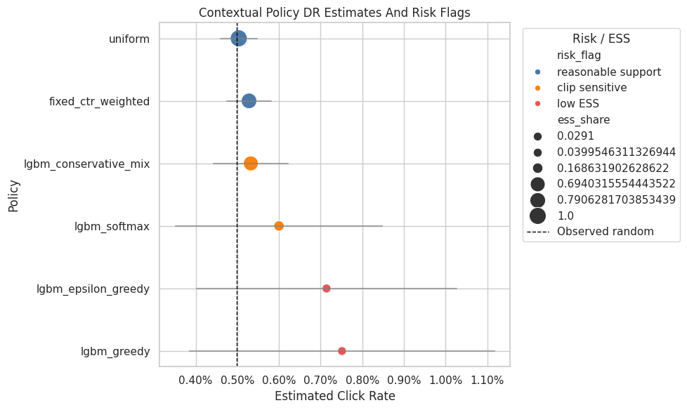

PosixPath('/home/apex/Documents/ranking_sys/notebooks/projects/project_2_off_policy_evaluation/writeup/figures/02_contextual_policy_value_and_risk.png')

This figure turns the final OPE results into a visual artifact for the writeup. The plot should be read together with support and sensitivity tables, not as a standalone proof that a policy will win online.

Figure 3: Lift Versus Effective Sample Size

This figure plots estimated DR lift against effective sample size share.

This is one of the clearest final-report visuals because it shows the policy tradeoff directly. A policy in the upper-right is attractive: high lift and strong support. A policy in the upper-left may be promising but fragile.

fig, ax = plt.subplots(figsize=(9, 6))
sns.scatterplot(
    data=contextual_final,
    x="ess_share",
    y="lift_pp",
    hue="risk_flag",
    size="max_weight",
    sizes=(60, 260),
    palette=palette,
    ax=ax,
)
for _, row in contextual_final.iterrows():
    ax.text(row["ess_share"] + 0.01, row["lift_pp"], row["policy"], fontsize=9)
ax.axhline(0, color="black", linestyle="--", linewidth=1)
ax.set_title("Policy Lift Versus Support")
ax.set_xlabel("Effective Sample Size Share")
ax.set_ylabel("DR Lift vs Random, percentage points")
ax.xaxis.set_major_formatter(lambda x, _: f"{x:.0%}")
ax.legend(title="Risk / max weight", bbox_to_anchor=(1.02, 1), loc="upper left")
plt.tight_layout()

support_lift_figure = FIGURE_DIR / "03_lift_vs_support.png"
fig.savefig(support_lift_figure, dpi=180, bbox_inches="tight")
plt.show()

support_lift_figure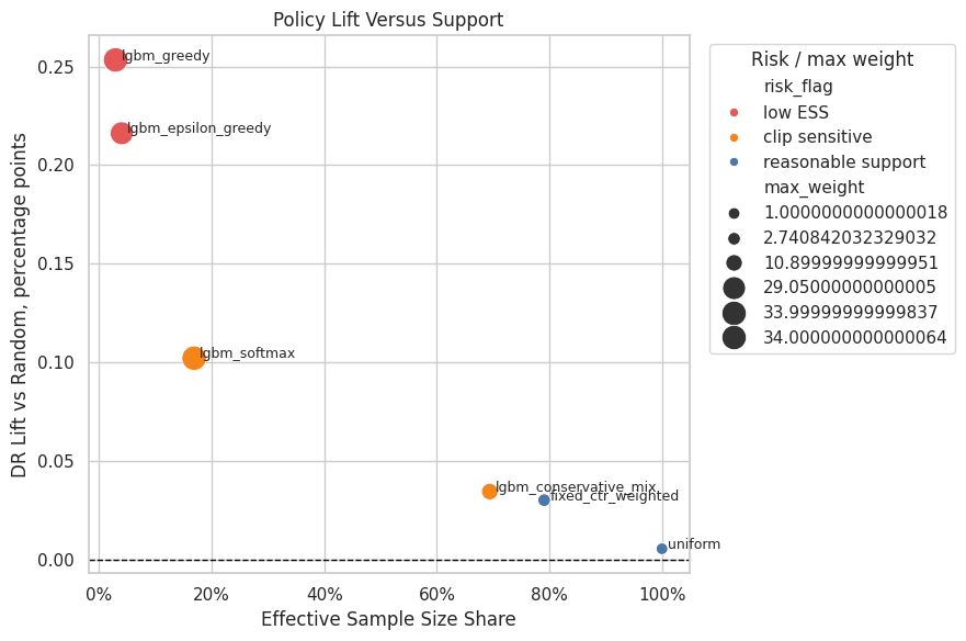

PosixPath('/home/apex/Documents/ranking_sys/notebooks/projects/project_2_off_policy_evaluation/writeup/figures/03_lift_vs_support.png')

Effective sample size turns weight concentration into an intuitive sample-size diagnostic. A low ESS means the estimator has less usable information than the raw row count suggests.

Figure 4: Clipping Sensitivity

This figure summarizes DR clipping sensitivity for contextual policies.

A large clipping range means the estimate changes when high weights are capped. That is a warning sign that the policy value depends on a small number of high-weight rows.

clipping_plot = contextual_clipping.sort_values("dr_estimate_range", ascending=True).copy()

fig, ax = plt.subplots(figsize=(9, 5))
sns.barplot(data=clipping_plot, x="dr_estimate_range", y="policy", color="#72B7B2", ax=ax)
ax.set_title("Contextual DR Estimate Sensitivity To Weight Clipping")
ax.set_xlabel("Range of DR estimates across clipping settings")
ax.set_ylabel("Policy")
ax.xaxis.set_major_formatter(lambda x, _: f"{x:.2%}")
plt.tight_layout()

clipping_figure = FIGURE_DIR / "04_contextual_clipping_sensitivity.png"
fig.savefig(clipping_figure, dpi=180, bbox_inches="tight")
plt.show()

clipping_figure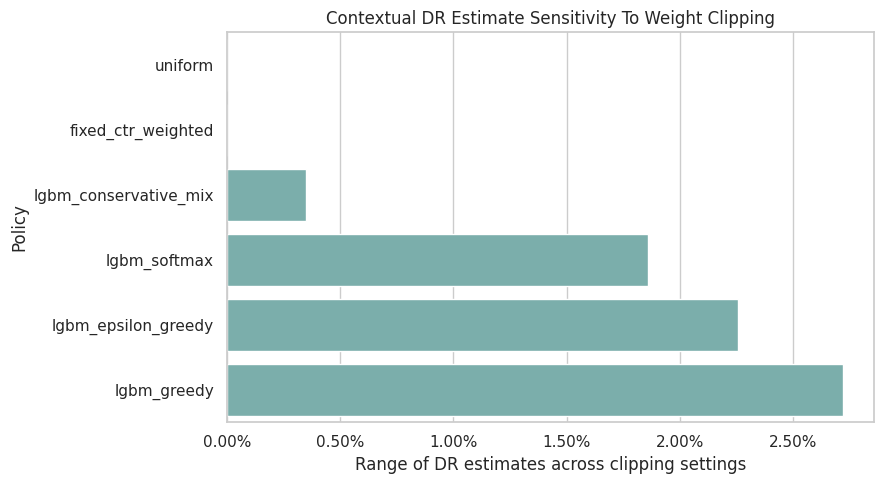

PosixPath('/home/apex/Documents/ranking_sys/notebooks/projects/project_2_off_policy_evaluation/writeup/figures/04_contextual_clipping_sensitivity.png')

The clipping sensitivity check shows how estimates change when extreme weights are capped. Stable estimates across clipping thresholds are more reassuring than estimates that depend strongly on a few high-weight rows.

Final Recommendation Table

This cell creates the final recommendation table.

The recommendation is deliberately split into two roles:

• a primary contextual candidate that uses personalization while preserving more support than a greedy policy
• a stable fixed-policy fallback that is simpler and has stronger support diagnostics

This framing is useful for interviews because it shows product judgment, not just model chasing.

primary_contextual = contextual_final.query("policy == 'lgbm_conservative_mix'").iloc[0]
stable_fixed = contextual_final.query("policy == 'fixed_ctr_weighted'").iloc[0]
aggressive_reference = contextual_final.query("policy == 'lgbm_greedy'").iloc[0]

final_recommendation = pd.DataFrame(
    [
        {
            "role": "primary A/B-test candidate",
            "policy": primary_contextual["policy"],
            "reason": "Context-aware policy with materially better support than greedy learned policies.",
            "estimated_click_rate": primary_contextual["estimate"],
            "lift_pp": primary_contextual["lift_pp"],
            "relative_lift_pct": primary_contextual["relative_lift_pct"],
            "ess_share": primary_contextual["ess_share"],
            "max_weight": primary_contextual["max_weight"],
            "risk_flag": primary_contextual["risk_flag"],
        },
        {
            "role": "stable fallback candidate",
            "policy": stable_fixed["policy"],
            "reason": "Simpler fixed policy with reasonable support and low clipping sensitivity.",
            "estimated_click_rate": stable_fixed["estimate"],
            "lift_pp": stable_fixed["lift_pp"],
            "relative_lift_pct": stable_fixed["relative_lift_pct"],
            "ess_share": stable_fixed["ess_share"],
            "max_weight": stable_fixed["max_weight"],
            "risk_flag": stable_fixed["risk_flag"],
        },
        {
            "role": "not recommended as first rollout",
            "policy": aggressive_reference["policy"],
            "reason": "High estimated value but very low ESS and high clipping sensitivity.",
            "estimated_click_rate": aggressive_reference["estimate"],
            "lift_pp": aggressive_reference["lift_pp"],
            "relative_lift_pct": aggressive_reference["relative_lift_pct"],
            "ess_share": aggressive_reference["ess_share"],
            "max_weight": aggressive_reference["max_weight"],
            "risk_flag": aggressive_reference["risk_flag"],
        },
    ]
)

final_recommendation_path = TABLE_DIR / "final_recommendation.csv"
final_recommendation.to_csv(final_recommendation_path, index=False)

final_recommendation

	role	policy	reason	estimated_click_rate	lift_pp	relative_lift_pct	ess_share	max_weight	risk_flag
0	primary A/B-test candidate	lgbm_conservative_mix	Context-aware policy with materially better su...	0.005324	0.034450	6.917631	0.694032	10.900000	clip sensitive
1	stable fallback candidate	fixed_ctr_weighted	Simpler fixed policy with reasonable support a...	0.005281	0.030119	6.048007	0.790628	2.740842	reasonable support
2	not recommended as first rollout	lgbm_greedy	High estimated value but very low ESS and high...	0.007513	0.253344	50.872251	0.029100	34.000000	low ESS

The final table distills the offline evidence into a small set of decision-relevant rows. This is the version most useful for a portfolio writeup or stakeholder-facing summary.

Limitations Table

This table lists the main limitations that should appear in the final writeup.

The limitations are part of the value of the project. In causal recommendation work, being explicit about support, logging propensities, short-term outcomes, and online validation makes the analysis more credible.

limitations = pd.DataFrame(
    [
        {
            "limitation": "Offline OPE is not an online experiment",
            "impact": "The estimates prioritize A/B-test candidates but do not prove production lift.",
            "mitigation": "Run an online experiment with guardrail metrics before launch.",
        },
        {
            "limitation": "Support and positivity constraints",
            "impact": "Aggressive learned policies can have low ESS and high weight sensitivity.",
            "mitigation": "Use conservative mixtures and monitor ESS, max weights, and clipping sensitivity.",
        },
        {
            "limitation": "Reward is short-term click",
            "impact": "Click lift may not equal long-term satisfaction, retention, or content discovery quality.",
            "mitigation": "Add downstream engagement and retention guardrails in online testing.",
        },
        {
            "limitation": "Reward-model dependence",
            "impact": "Direct method and DR estimates depend partly on model quality and calibration.",
            "mitigation": "Compare reward models, calibration, and residual correction diagnostics.",
        },
        {
            "limitation": "Single Open Bandit campaign slice",
            "impact": "The project focuses on the `random/men` slice for clarity and support.",
            "mitigation": "Extend to other campaigns or BTS logs as a robustness check.",
        },
    ]
)

limitations_path = TABLE_DIR / "limitations.csv"
limitations.to_csv(limitations_path, index=False)

limitations

	limitation	impact	mitigation
0	Offline OPE is not an online experiment	The estimates prioritize A/B-test candidates b...	Run an online experiment with guardrail metric...
1	Support and positivity constraints	Aggressive learned policies can have low ESS a...	Use conservative mixtures and monitor ESS, max...
2	Reward is short-term click	Click lift may not equal long-term satisfactio...	Add downstream engagement and retention guardr...
3	Reward-model dependence	Direct method and DR estimates depend partly o...	Compare reward models, calibration, and residu...
4	Single Open Bandit campaign slice	The project focuses on the `random/men` slice ...	Extend to other campaigns or BTS logs as a rob...

The limitations table states what the offline analysis cannot guarantee. This is a strength of the project: it shows judgment about support, unobserved confounding, logging assumptions, and the need for online validation.

Final Portfolio Summary Text

This cell writes a concise project summary that can be reused in a README, portfolio page, or interview prep notes.

The wording is intentionally careful: it describes the policy as an offline A/B-test candidate rather than claiming production causality.

summary_text = f"""# Final Summary: Off-Policy Evaluation Of Recommendation Systems

## Problem
This project evaluates recommendation policies offline using logged bandit data. The business question is: which recommendation policy is most credible to advance to an online A/B test?

## Dataset
The analysis uses the Open Bandit Dataset, focusing on the `random/men` campaign because it contains logged actions, click rewards, context features, and known behavior-policy propensities. The random behavior policy provides broad support, which is important for reliable off-policy evaluation.

## Methods
The project implements IPS, self-normalized IPS, direct method, doubly robust OPE, weight diagnostics, reward-model diagnostics, clipping sensitivity, reward-model sensitivity, split sensitivity, and contextual policy learning with LightGBM reward scores.

## Final Recommendation
The primary offline A/B-test candidate is `{primary_contextual['policy']}`. Its estimated DR click rate is {primary_contextual['estimate']:.4%}, with estimated lift of {primary_contextual['lift_pp']:.3f} percentage points versus the observed random-policy baseline. Because this policy is still marked `{primary_contextual['risk_flag']}`, the safer fallback is `{stable_fixed['policy']}`, which has stronger support diagnostics and estimated lift of {stable_fixed['lift_pp']:.3f} percentage points.

## Interpretation
The project does not claim that offline OPE proves production impact. It recommends a prioritized online experiment: test a conservative contextual policy or stable fixed policy against the current/random baseline, while tracking click quality, longer-term engagement, and user experience guardrails.
""".strip()

summary_path = WRITEUP_DIR / "final_project_summary.md"
summary_path.write_text(summary_text + "\n")

print(summary_text)

# Final Summary: Off-Policy Evaluation Of Recommendation Systems

## Problem
This project evaluates recommendation policies offline using logged bandit data. The business question is: which recommendation policy is most credible to advance to an online A/B test?

## Dataset
The analysis uses the Open Bandit Dataset, focusing on the `random/men` campaign because it contains logged actions, click rewards, context features, and known behavior-policy propensities. The random behavior policy provides broad support, which is important for reliable off-policy evaluation.

## Methods
The project implements IPS, self-normalized IPS, direct method, doubly robust OPE, weight diagnostics, reward-model diagnostics, clipping sensitivity, reward-model sensitivity, split sensitivity, and contextual policy learning with LightGBM reward scores.

## Final Recommendation
The primary offline A/B-test candidate is `lgbm_conservative_mix`. Its estimated DR click rate is 0.5324%, with estimated lift of 0.034 percentage points versus the observed random-policy baseline. Because this policy is still marked `clip sensitive`, the safer fallback is `fixed_ctr_weighted`, which has stronger support diagnostics and estimated lift of 0.030 percentage points.

## Interpretation
The project does not claim that offline OPE proves production impact. It recommends a prioritized online experiment: test a conservative contextual policy or stable fixed policy against the current/random baseline, while tracking click quality, longer-term engagement, and user experience guardrails.

This cell saves reusable outputs for downstream notebooks or the final writeup. Persisting these artifacts makes the project modular and prevents later notebooks from repeating expensive or fragile setup work.

Resume Bullets

This cell writes resume-ready bullets for data science roles.

The bullets are specific enough to show technical substance and product relevance. They mention OPE, recommendation systems, propensities, doubly robust estimation, and contextual policy learning.

resume_bullets = f"""# Resume Bullets

- Built an off-policy evaluation framework for recommendation systems using Open Bandit logs, estimating counterfactual policy value with IPS, self-normalized IPS, direct method, and doubly robust estimators from logged propensities.
- Trained LightGBM reward models to learn context-aware recommendation policies, then evaluated greedy, epsilon-greedy, softmax, and conservative mixed policies with ESS, clipping sensitivity, and residual-correction diagnostics.
- Produced an A/B-test recommendation framework that balanced estimated click lift with support risk, identifying `{primary_contextual['policy']}` as a contextual candidate and `{stable_fixed['policy']}` as a stable fallback policy.
""".strip()

resume_path = WRITEUP_DIR / "resume_bullets.md"
resume_path.write_text(resume_bullets + "\n")

print(resume_bullets)

# Resume Bullets

- Built an off-policy evaluation framework for recommendation systems using Open Bandit logs, estimating counterfactual policy value with IPS, self-normalized IPS, direct method, and doubly robust estimators from logged propensities.
- Trained LightGBM reward models to learn context-aware recommendation policies, then evaluated greedy, epsilon-greedy, softmax, and conservative mixed policies with ESS, clipping sensitivity, and residual-correction diagnostics.
- Produced an A/B-test recommendation framework that balanced estimated click lift with support risk, identifying `lgbm_conservative_mix` as a contextual candidate and `fixed_ctr_weighted` as a stable fallback policy.

This cell saves reusable outputs for downstream notebooks or the final writeup. Persisting these artifacts makes the project modular and prevents later notebooks from repeating expensive or fragile setup work.

Final Artifact Index

This final cell lists the files generated for the off-policy evaluation writeup.

The artifact index is useful because the project now has several notebooks and many generated files. This table tells you exactly which figures, tables, and markdown snippets are ready for the README or portfolio page.

artifact_paths = sorted(
    [path for path in WRITEUP_DIR.rglob("*") if path.is_file()]
)
artifact_index = pd.DataFrame(
    {
        "path": [str(path.relative_to(PROJECT_ROOT)) for path in artifact_paths],
        "size_kb": [path.stat().st_size / 1024 for path in artifact_paths],
    }
)

artifact_index_path = TABLE_DIR / "artifact_index.csv"
artifact_index.to_csv(artifact_index_path, index=False)

artifact_index

	path	size_kb
0	notebooks/projects/project_2_off_policy_evaluation/writeup/figure...	111.525391
1	notebooks/projects/project_2_off_policy_evaluation/writeup/figure...	144.845703
2	notebooks/projects/project_2_off_policy_evaluation/writeup/figure...	142.990234
3	notebooks/projects/project_2_off_policy_evaluation/writeup/figure...	70.702148
4	notebooks/projects/project_2_off_policy_evaluation/writeup/final_...	1.539062
5	notebooks/projects/project_2_off_policy_evaluation/writeup/resume...	0.683594
6	notebooks/projects/project_2_off_policy_evaluation/writeup/tables...	1.283203
7	notebooks/projects/project_2_off_policy_evaluation/writeup/tables...	0.702148
8	notebooks/projects/project_2_off_policy_evaluation/writeup/tables...	0.830078
9	notebooks/projects/project_2_off_policy_evaluation/writeup/tables...	1.428711
10	notebooks/projects/project_2_off_policy_evaluation/writeup/tables...	6.987305
11	notebooks/projects/project_2_off_policy_evaluation/writeup/tables...	1.569336
12	notebooks/projects/project_2_off_policy_evaluation/writeup/tables...	0.751953
13	notebooks/projects/project_2_off_policy_evaluation/writeup/tables...	0.915039
14	notebooks/projects/project_2_off_policy_evaluation/writeup/tables...	4.750000
15	notebooks/projects/project_2_off_policy_evaluation/writeup/tables...	1.785156
16	notebooks/projects/project_2_off_policy_evaluation/writeup/tables...	0.300781
17	notebooks/projects/project_2_off_policy_evaluation/writeup/tables...	0.527344

This cell saves reusable outputs for downstream notebooks or the final writeup. Persisting these artifacts makes the project modular and prevents later notebooks from repeating expensive or fragile setup work.

Notebook 7 Takeaways

The off-policy evaluation work is now packaged as a complete portfolio project.

The final outputs include:

• method timeline
• fixed-policy OPE comparison
• contextual-policy decision table
• lift versus support figure
• clipping sensitivity figure
• final recommendation table
• limitations table
• project summary markdown
• resume bullets
• artifact index

The project has a complete technical arc: it starts from logged bandit data, validates propensities and support, implements classical and doubly robust OPE, stress-tests policy conclusions, learns contextual policies, and ends with a cautious A/B-test recommendation.