06 Contextual Policy Learning

This notebook is the advanced modeling notebook for Off-Policy Evaluation of Recommendation Systems.

The earlier notebooks evaluated simple policies that assigned the same item probabilities for every user/context. That was useful for learning IPS, SNIPS, direct method, and doubly robust OPE, but real recommendation systems are contextual. A production recommendation policy should change its item choices based on user features, time, position, and item-user affinity signals.

This notebook asks:

Can we learn a context-aware recommendation policy from logged data, then evaluate it offline with OPE?

We train reward models, score every held-out context against every candidate item, convert those scores into contextual policies, and evaluate those policies with IPS, SNIPS, direct method, and doubly robust estimation.

Why Contextual Policy Learning?

A fixed policy says, for example, “recommend item 7 with 20% probability for everyone.” That is easy to evaluate, but it ignores personalization.

A contextual policy says, “for this user and this context, choose the item with the best predicted reward distribution.” This is closer to real recommendation systems because the policy can adapt to:

• user features
• time of day
• recommendation position
• item metadata
• user-item affinity signals

The danger is that learned contextual policies can become aggressive. A fully greedy policy may put all probability on one predicted-best item per context. If the behavior policy rarely logged that item for similar contexts, IPS and DR corrections can become noisy. This notebook therefore compares aggressive and conservative learned policies.

Notebook Setup

This cell imports the libraries used for reward modeling, policy learning, OPE, and plotting.

It also suppresses one known LightGBM/sklearn metadata warning about feature names. That warning appears when LightGBM is used inside a scikit-learn pipeline and does not indicate a modeling problem. The filter is targeted so other warnings remain visible.

from pathlib import Path
import warnings

import lightgbm as lgb
import matplotlib.pyplot as plt
import numpy as np
import pandas as pd
import seaborn as sns
from sklearn.compose import ColumnTransformer
from sklearn.linear_model import LogisticRegression
from sklearn.metrics import average_precision_score, brier_score_loss, log_loss, roc_auc_score
from sklearn.pipeline import Pipeline
from sklearn.preprocessing import OneHotEncoder, StandardScaler

pd.set_option("display.max_columns", 140)
pd.set_option("display.max_rows", 140)
pd.set_option("display.float_format", "{:.6f}".format)

sns.set_theme(style="whitegrid", context="notebook")

warnings.filterwarnings(
    "ignore",
    message="X does not have valid feature names, but LGBMClassifier was fitted with feature names",
    category=UserWarning,
)

This cell prepares the notebook environment for contextual policy learning with offline evaluation. There is no estimator output yet; the main value is that the imports, display settings, and plotting defaults are ready for the OPE diagnostics that follow.

Load The Random Open Bandit Sample

This cell loads the same random/men sample used throughout the OPE project.

The random behavior policy is valuable here because it gives broad action support. Contextual policies can be more concentrated than fixed policies, so a randomized log is the safest place to evaluate them offline.

RANDOM_SAMPLE_RELATIVE_PATH = Path("data/processed/open_bandit_random_men_sample.parquet")
PROJECT_ROOT = next(
    path
    for path in [Path.cwd(), *Path.cwd().parents]
    if (path / RANDOM_SAMPLE_RELATIVE_PATH).exists()
)

RANDOM_SAMPLE_PATH = PROJECT_ROOT / RANDOM_SAMPLE_RELATIVE_PATH
random_df = pd.read_parquet(RANDOM_SAMPLE_PATH).sort_values("timestamp").reset_index(drop=True)

pd.Series(
    {
        "project_root": PROJECT_ROOT,
        "random_sample_path": RANDOM_SAMPLE_PATH,
        "rows": len(random_df),
        "columns": random_df.shape[1],
        "observed_click_rate": random_df["click"].mean(),
    }
).to_frame("value")

	value
project_root	/home/apex/Documents/ranking_sys
random_sample_path	/home/apex/Documents/ranking_sys/data/processe...
rows	200000
columns	50
observed_click_rate	0.005190

The loaded table shape and preview confirm that the expected cached data is available. This check matters because all later OPE estimates depend on using the correct logged actions, rewards, contexts, and behavior propensities.

Create Train And Evaluation Splits

This notebook uses the same primary time split as the previous OPE notebooks.

The training split is used to fit reward models and define learned policies. The evaluation split is used for off-policy evaluation. This keeps policy learning separate from policy evaluation and reduces the risk of overclaiming from in-sample performance.

SPLIT_FRACTION = 0.50
split_idx = int(len(random_df) * SPLIT_FRACTION)

train_df = random_df.iloc[:split_idx].copy()
eval_df = random_df.iloc[split_idx:].copy()

split_summary = pd.DataFrame(
    {
        "split": ["train", "evaluation"],
        "rows": [len(train_df), len(eval_df)],
        "min_timestamp": [train_df["timestamp"].min(), eval_df["timestamp"].min()],
        "max_timestamp": [train_df["timestamp"].max(), eval_df["timestamp"].max()],
        "click_rate": [train_df["click"].mean(), eval_df["click"].mean()],
    }
)

split_summary

	split	rows	min_timestamp	max_timestamp	click_rate
0	train	100000	2019-11-24 00:00:03.800821+00:00	2019-11-25 10:01:18.392921+00:00	0.005400
1	evaluation	100000	2019-11-25 10:01:18.393450+00:00	2019-11-27 02:50:16.027289+00:00	0.004980

The split separates policy construction from policy evaluation. This prevents using the same rows to design a policy and evaluate it, which would make the offline result too optimistic.

Define Feature Groups And Action Space

This cell defines the action space and model feature groups.

The action is item_id. The reward model uses user features, item features, position, hour, and a selected affinity feature. The selected affinity feature is built by choosing the user-item affinity column that corresponds to the candidate item being scored.

action_space = np.array(sorted(random_df["item_id"].unique()))
n_actions = len(action_space)

action_to_index = {item_id: idx for idx, item_id in enumerate(action_space)}
user_feature_cols = [col for col in random_df.columns if col.startswith("user_feature_")]
affinity_cols_by_action = [f"user-item_affinity_{item_id}" for item_id in action_space]
item_feature_cols = [col for col in random_df.columns if col.startswith("item_feature_")]

categorical_features = [
    "position",
    "hour",
    "item_id",
    *user_feature_cols,
    "item_feature_1",
    "item_feature_2",
    "item_feature_3",
]
numeric_features = ["selected_affinity", "item_feature_0"]
feature_cols = categorical_features + numeric_features

feature_summary = pd.DataFrame(
    {
        "group": ["actions", "user features", "affinity columns", "item features", "model categorical", "model numeric"],
        "count": [n_actions, len(user_feature_cols), len(affinity_cols_by_action), len(item_feature_cols), len(categorical_features), len(numeric_features)],
    }
)

feature_summary

	group	count
0	actions	34
1	user features	4
2	affinity columns	34
3	item features	4
4	model categorical	10
5	model numeric	2

The action-space definition fixes the set of items that evaluation policies are allowed to choose. OPE estimates are only meaningful for policies whose action probabilities live inside this logged support.

Build Item Metadata Lookup

The cached sample contains item metadata for the logged item. To score counterfactual candidate items, we need item metadata for every candidate item.

This cell builds a one-row-per-item lookup table. When we score candidate item a, we attach the metadata for a, regardless of which item was actually logged in that row.

item_context = (
    random_df[["item_id", *item_feature_cols]]
    .drop_duplicates("item_id")
    .set_index("item_id")
    .sort_index()
)

missing_items = sorted(set(action_space) - set(item_context.index))
if missing_items:
    raise ValueError(f"Missing item metadata for item IDs: {missing_items}")

item_context.head()

	item_feature_0	item_feature_1	item_feature_2	item_feature_3
item_id
0	-0.677183	ce58bf66d7e62186e6ce01bafeea9d39	7c5498711d69681385d21c0e26923e7e	bbf748c6c978938bc63d432efa60191c
1	-0.720300	3c2985d744e0d57c261abd7e541e4263	7c5498711d69681385d21c0e26923e7e	bbf748c6c978938bc63d432efa60191c
2	0.745662	3c2985d744e0d57c261abd7e541e4263	2b851c0a9c4a961da8760d5dc747c5a3	b61cfaadd526b816e3aeb9b7be4b4759
3	-0.698741	9874ffb54e9b0a269e29bbb2f5328735	ce1abd8b5d914ba8fe719b453bc5ba3b	5bc9c86cd1f08a9991670ea97b34f86d
4	1.651109	01fe2f187e459e6ada960671d2942dfe	b4b5879029fb5f64eeec63cf4f73ef0e	b61cfaadd526b816e3aeb9b7be4b4759

These feature-building cells define the context used by reward models. Reward models need both user context and candidate item context so they can predict counterfactual rewards for actions that were not logged.

Define Feature Builders

This cell defines two feature builders.

make_logged_feature_frame creates features for the item actually shown in each logged row. This is used to train and evaluate reward models on observed outcomes.

make_candidate_feature_frame creates features for every candidate item in each context. This is used to learn contextual policies and compute direct-method components.

def make_logged_feature_frame(df):
    """Create model features for the logged action in each row."""
    frame = df.copy()
    affinity_matrix = frame[affinity_cols_by_action].to_numpy()
    item_positions = frame["item_id"].map(action_to_index).to_numpy()
    frame["selected_affinity"] = affinity_matrix[np.arange(len(frame)), item_positions]
    return frame[feature_cols]


def make_candidate_feature_frame(context_df):
    """Create model features for every candidate action in each context row."""
    n_contexts = len(context_df)
    tiled_actions = np.tile(action_space, n_contexts)

    frame = pd.DataFrame(
        {
            "position": np.repeat(context_df["position"].to_numpy(), n_actions),
            "hour": np.repeat(context_df["hour"].to_numpy(), n_actions),
            "item_id": tiled_actions,
        }
    )

    for col in user_feature_cols:
        frame[col] = np.repeat(context_df[col].to_numpy(), n_actions)

    affinity_matrix = context_df[affinity_cols_by_action].to_numpy()
    frame["selected_affinity"] = affinity_matrix.reshape(-1)

    repeated_item_context = item_context.loc[tiled_actions, item_feature_cols].reset_index(drop=True)
    frame = pd.concat([frame, repeated_item_context], axis=1)

    return frame[feature_cols]

make_candidate_feature_frame(eval_df.head(2))

	position	hour	item_id	user_feature_0	user_feature_1	user_feature_2	user_feature_3	item_feature_1	item_feature_2	item_feature_3	selected_affinity	item_feature_0
0	2	10	0	cef3390ed299c09874189c387777674a	2d03db5543b14483e52d761760686b64	2723d2eb8bba04e0362098011fa3997b	9bde591ffaab8d54c457448e4dca6f53	ce58bf66d7e62186e6ce01bafeea9d39	7c5498711d69681385d21c0e26923e7e	bbf748c6c978938bc63d432efa60191c	0.000000	-0.677183
1	2	10	1	cef3390ed299c09874189c387777674a	2d03db5543b14483e52d761760686b64	2723d2eb8bba04e0362098011fa3997b	9bde591ffaab8d54c457448e4dca6f53	3c2985d744e0d57c261abd7e541e4263	7c5498711d69681385d21c0e26923e7e	bbf748c6c978938bc63d432efa60191c	0.000000	-0.720300
2	2	10	2	cef3390ed299c09874189c387777674a	2d03db5543b14483e52d761760686b64	2723d2eb8bba04e0362098011fa3997b	9bde591ffaab8d54c457448e4dca6f53	3c2985d744e0d57c261abd7e541e4263	2b851c0a9c4a961da8760d5dc747c5a3	b61cfaadd526b816e3aeb9b7be4b4759	0.000000	0.745662
3	2	10	3	cef3390ed299c09874189c387777674a	2d03db5543b14483e52d761760686b64	2723d2eb8bba04e0362098011fa3997b	9bde591ffaab8d54c457448e4dca6f53	9874ffb54e9b0a269e29bbb2f5328735	ce1abd8b5d914ba8fe719b453bc5ba3b	5bc9c86cd1f08a9991670ea97b34f86d	0.000000	-0.698741
4	2	10	4	cef3390ed299c09874189c387777674a	2d03db5543b14483e52d761760686b64	2723d2eb8bba04e0362098011fa3997b	9bde591ffaab8d54c457448e4dca6f53	01fe2f187e459e6ada960671d2942dfe	b4b5879029fb5f64eeec63cf4f73ef0e	b61cfaadd526b816e3aeb9b7be4b4759	0.000000	1.651109
5	2	10	5	cef3390ed299c09874189c387777674a	2d03db5543b14483e52d761760686b64	2723d2eb8bba04e0362098011fa3997b	9bde591ffaab8d54c457448e4dca6f53	01fe2f187e459e6ada960671d2942dfe	c43671ed6855a6fe2e2a6030cba64366	bbf748c6c978938bc63d432efa60191c	0.000000	0.142031
6	2	10	6	cef3390ed299c09874189c387777674a	2d03db5543b14483e52d761760686b64	2723d2eb8bba04e0362098011fa3997b	9bde591ffaab8d54c457448e4dca6f53	ce58bf66d7e62186e6ce01bafeea9d39	7082af732502f0981a9fe77d7ba1ae8a	b61cfaadd526b816e3aeb9b7be4b4759	0.000000	1.651109
7	2	10	7	cef3390ed299c09874189c387777674a	2d03db5543b14483e52d761760686b64	2723d2eb8bba04e0362098011fa3997b	9bde591ffaab8d54c457448e4dca6f53	01fe2f187e459e6ada960671d2942dfe	2b851c0a9c4a961da8760d5dc747c5a3	b61cfaadd526b816e3aeb9b7be4b4759	0.000000	2.858372
8	2	10	8	cef3390ed299c09874189c387777674a	2d03db5543b14483e52d761760686b64	2723d2eb8bba04e0362098011fa3997b	9bde591ffaab8d54c457448e4dca6f53	01fe2f187e459e6ada960671d2942dfe	d7f03898d040700d6e1810d21e669958	b61cfaadd526b816e3aeb9b7be4b4759	0.000000	1.349294
9	2	10	9	cef3390ed299c09874189c387777674a	2d03db5543b14483e52d761760686b64	2723d2eb8bba04e0362098011fa3997b	9bde591ffaab8d54c457448e4dca6f53	9874ffb54e9b0a269e29bbb2f5328735	2b851c0a9c4a961da8760d5dc747c5a3	b61cfaadd526b816e3aeb9b7be4b4759	0.000000	1.198386
10	2	10	10	cef3390ed299c09874189c387777674a	2d03db5543b14483e52d761760686b64	2723d2eb8bba04e0362098011fa3997b	9bde591ffaab8d54c457448e4dca6f53	9874ffb54e9b0a269e29bbb2f5328735	2b851c0a9c4a961da8760d5dc747c5a3	b61cfaadd526b816e3aeb9b7be4b4759	0.000000	1.586435
11	2	10	11	cef3390ed299c09874189c387777674a	2d03db5543b14483e52d761760686b64	2723d2eb8bba04e0362098011fa3997b	9bde591ffaab8d54c457448e4dca6f53	ce58bf66d7e62186e6ce01bafeea9d39	eddad9910a6d2f61905f408d4df575c5	de8b129010093b09b24a05592bfd8843	0.000000	0.443847
12	2	10	12	cef3390ed299c09874189c387777674a	2d03db5543b14483e52d761760686b64	2723d2eb8bba04e0362098011fa3997b	9bde591ffaab8d54c457448e4dca6f53	ce58bf66d7e62186e6ce01bafeea9d39	697cbf60c7c4b8569c149721231538c3	b61cfaadd526b816e3aeb9b7be4b4759	0.000000	1.198386
13	2	10	13	cef3390ed299c09874189c387777674a	2d03db5543b14483e52d761760686b64	2723d2eb8bba04e0362098011fa3997b	9bde591ffaab8d54c457448e4dca6f53	9874ffb54e9b0a269e29bbb2f5328735	697cbf60c7c4b8569c149721231538c3	b61cfaadd526b816e3aeb9b7be4b4759	0.000000	0.616313
14	2	10	14	cef3390ed299c09874189c387777674a	2d03db5543b14483e52d761760686b64	2723d2eb8bba04e0362098011fa3997b	9bde591ffaab8d54c457448e4dca6f53	9874ffb54e9b0a269e29bbb2f5328735	3f1feafd79578bedf199c459fecc378b	bbf748c6c978938bc63d432efa60191c	0.000000	-1.000557
15	2	10	15	cef3390ed299c09874189c387777674a	2d03db5543b14483e52d761760686b64	2723d2eb8bba04e0362098011fa3997b	9bde591ffaab8d54c457448e4dca6f53	ce58bf66d7e62186e6ce01bafeea9d39	9f9ff361c09f765650f1c43ef7adac86	5bc9c86cd1f08a9991670ea97b34f86d	0.000000	-0.375367
16	2	10	16	cef3390ed299c09874189c387777674a	2d03db5543b14483e52d761760686b64	2723d2eb8bba04e0362098011fa3997b	9bde591ffaab8d54c457448e4dca6f53	ce58bf66d7e62186e6ce01bafeea9d39	5d5dd3635cb3f84d3a70f5874a132d44	5bc9c86cd1f08a9991670ea97b34f86d	0.000000	-0.590950
17	2	10	17	cef3390ed299c09874189c387777674a	2d03db5543b14483e52d761760686b64	2723d2eb8bba04e0362098011fa3997b	9bde591ffaab8d54c457448e4dca6f53	9874ffb54e9b0a269e29bbb2f5328735	5d5dd3635cb3f84d3a70f5874a132d44	5bc9c86cd1f08a9991670ea97b34f86d	0.000000	-0.698741
18	2	10	18	cef3390ed299c09874189c387777674a	2d03db5543b14483e52d761760686b64	2723d2eb8bba04e0362098011fa3997b	9bde591ffaab8d54c457448e4dca6f53	3c2985d744e0d57c261abd7e541e4263	5d5dd3635cb3f84d3a70f5874a132d44	5bc9c86cd1f08a9991670ea97b34f86d	0.000000	-0.914324
19	2	10	19	cef3390ed299c09874189c387777674a	2d03db5543b14483e52d761760686b64	2723d2eb8bba04e0362098011fa3997b	9bde591ffaab8d54c457448e4dca6f53	3c2985d744e0d57c261abd7e541e4263	5d5dd3635cb3f84d3a70f5874a132d44	5bc9c86cd1f08a9991670ea97b34f86d	0.000000	-0.763416
20	2	10	20	cef3390ed299c09874189c387777674a	2d03db5543b14483e52d761760686b64	2723d2eb8bba04e0362098011fa3997b	9bde591ffaab8d54c457448e4dca6f53	3c2985d744e0d57c261abd7e541e4263	5d5dd3635cb3f84d3a70f5874a132d44	5bc9c86cd1f08a9991670ea97b34f86d	0.000000	-0.612508
21	2	10	21	cef3390ed299c09874189c387777674a	2d03db5543b14483e52d761760686b64	2723d2eb8bba04e0362098011fa3997b	9bde591ffaab8d54c457448e4dca6f53	9874ffb54e9b0a269e29bbb2f5328735	ce1abd8b5d914ba8fe719b453bc5ba3b	5bc9c86cd1f08a9991670ea97b34f86d	0.000000	-0.698741
22	2	10	22	cef3390ed299c09874189c387777674a	2d03db5543b14483e52d761760686b64	2723d2eb8bba04e0362098011fa3997b	9bde591ffaab8d54c457448e4dca6f53	61c5d8c2524684aa047e15e172c7e92f	7c5498711d69681385d21c0e26923e7e	bbf748c6c978938bc63d432efa60191c	0.000000	-0.698741
23	2	10	23	cef3390ed299c09874189c387777674a	2d03db5543b14483e52d761760686b64	2723d2eb8bba04e0362098011fa3997b	9bde591ffaab8d54c457448e4dca6f53	55fe518d85813954c7d9b8a875ff2453	cc75031396a5aa830885915aa93f49d0	b61cfaadd526b816e3aeb9b7be4b4759	0.000000	-0.569392
24	2	10	24	cef3390ed299c09874189c387777674a	2d03db5543b14483e52d761760686b64	2723d2eb8bba04e0362098011fa3997b	9bde591ffaab8d54c457448e4dca6f53	e95f0d1a3591e01d7ed3f0710424e84d	d7f03898d040700d6e1810d21e669958	b61cfaadd526b816e3aeb9b7be4b4759	0.000000	0.422288
25	2	10	25	cef3390ed299c09874189c387777674a	2d03db5543b14483e52d761760686b64	2723d2eb8bba04e0362098011fa3997b	9bde591ffaab8d54c457448e4dca6f53	9874ffb54e9b0a269e29bbb2f5328735	7c5498711d69681385d21c0e26923e7e	bbf748c6c978938bc63d432efa60191c	0.000000	-0.461600
26	2	10	26	cef3390ed299c09874189c387777674a	2d03db5543b14483e52d761760686b64	2723d2eb8bba04e0362098011fa3997b	9bde591ffaab8d54c457448e4dca6f53	3c2985d744e0d57c261abd7e541e4263	a86ead010f033dbc2854c6a46f4fe7a7	b61cfaadd526b816e3aeb9b7be4b4759	0.000000	0.896570
27	2	10	27	cef3390ed299c09874189c387777674a	2d03db5543b14483e52d761760686b64	2723d2eb8bba04e0362098011fa3997b	9bde591ffaab8d54c457448e4dca6f53	61c5d8c2524684aa047e15e172c7e92f	5d5dd3635cb3f84d3a70f5874a132d44	5bc9c86cd1f08a9991670ea97b34f86d	0.000000	-0.849649
28	2	10	28	cef3390ed299c09874189c387777674a	2d03db5543b14483e52d761760686b64	2723d2eb8bba04e0362098011fa3997b	9bde591ffaab8d54c457448e4dca6f53	61c5d8c2524684aa047e15e172c7e92f	b726ac74a20945400f27294febd4ab55	5bc9c86cd1f08a9991670ea97b34f86d	0.000000	-1.065232
29	2	10	29	cef3390ed299c09874189c387777674a	2d03db5543b14483e52d761760686b64	2723d2eb8bba04e0362098011fa3997b	9bde591ffaab8d54c457448e4dca6f53	61c5d8c2524684aa047e15e172c7e92f	7c63a6aa72e655abd1787c2e64385e6f	bbf748c6c978938bc63d432efa60191c	0.000000	-0.849649
30	2	10	30	cef3390ed299c09874189c387777674a	2d03db5543b14483e52d761760686b64	2723d2eb8bba04e0362098011fa3997b	9bde591ffaab8d54c457448e4dca6f53	61c5d8c2524684aa047e15e172c7e92f	3f1feafd79578bedf199c459fecc378b	bbf748c6c978938bc63d432efa60191c	0.000000	-0.914324
31	2	10	31	cef3390ed299c09874189c387777674a	2d03db5543b14483e52d761760686b64	2723d2eb8bba04e0362098011fa3997b	9bde591ffaab8d54c457448e4dca6f53	55fe518d85813954c7d9b8a875ff2453	7c63a6aa72e655abd1787c2e64385e6f	bbf748c6c978938bc63d432efa60191c	0.000000	-0.461600
32	2	10	32	cef3390ed299c09874189c387777674a	2d03db5543b14483e52d761760686b64	2723d2eb8bba04e0362098011fa3997b	9bde591ffaab8d54c457448e4dca6f53	e95f0d1a3591e01d7ed3f0710424e84d	b726ac74a20945400f27294febd4ab55	5bc9c86cd1f08a9991670ea97b34f86d	0.000000	-0.526275
33	2	10	33	cef3390ed299c09874189c387777674a	2d03db5543b14483e52d761760686b64	2723d2eb8bba04e0362098011fa3997b	9bde591ffaab8d54c457448e4dca6f53	e95f0d1a3591e01d7ed3f0710424e84d	7c5498711d69681385d21c0e26923e7e	bbf748c6c978938bc63d432efa60191c	0.000000	-0.612508
34	2	10	0	cef3390ed299c09874189c387777674a	03a5648a76832f83c859d46bc06cb64a	9b2d331c329ceb74d3dcfb48d8798c78	f97571b9c14a786aab269f0b427d2a85	ce58bf66d7e62186e6ce01bafeea9d39	7c5498711d69681385d21c0e26923e7e	bbf748c6c978938bc63d432efa60191c	0.000000	-0.677183
35	2	10	1	cef3390ed299c09874189c387777674a	03a5648a76832f83c859d46bc06cb64a	9b2d331c329ceb74d3dcfb48d8798c78	f97571b9c14a786aab269f0b427d2a85	3c2985d744e0d57c261abd7e541e4263	7c5498711d69681385d21c0e26923e7e	bbf748c6c978938bc63d432efa60191c	0.000000	-0.720300
36	2	10	2	cef3390ed299c09874189c387777674a	03a5648a76832f83c859d46bc06cb64a	9b2d331c329ceb74d3dcfb48d8798c78	f97571b9c14a786aab269f0b427d2a85	3c2985d744e0d57c261abd7e541e4263	2b851c0a9c4a961da8760d5dc747c5a3	b61cfaadd526b816e3aeb9b7be4b4759	0.000000	0.745662
37	2	10	3	cef3390ed299c09874189c387777674a	03a5648a76832f83c859d46bc06cb64a	9b2d331c329ceb74d3dcfb48d8798c78	f97571b9c14a786aab269f0b427d2a85	9874ffb54e9b0a269e29bbb2f5328735	ce1abd8b5d914ba8fe719b453bc5ba3b	5bc9c86cd1f08a9991670ea97b34f86d	0.000000	-0.698741
38	2	10	4	cef3390ed299c09874189c387777674a	03a5648a76832f83c859d46bc06cb64a	9b2d331c329ceb74d3dcfb48d8798c78	f97571b9c14a786aab269f0b427d2a85	01fe2f187e459e6ada960671d2942dfe	b4b5879029fb5f64eeec63cf4f73ef0e	b61cfaadd526b816e3aeb9b7be4b4759	0.000000	1.651109
39	2	10	5	cef3390ed299c09874189c387777674a	03a5648a76832f83c859d46bc06cb64a	9b2d331c329ceb74d3dcfb48d8798c78	f97571b9c14a786aab269f0b427d2a85	01fe2f187e459e6ada960671d2942dfe	c43671ed6855a6fe2e2a6030cba64366	bbf748c6c978938bc63d432efa60191c	0.000000	0.142031
40	2	10	6	cef3390ed299c09874189c387777674a	03a5648a76832f83c859d46bc06cb64a	9b2d331c329ceb74d3dcfb48d8798c78	f97571b9c14a786aab269f0b427d2a85	ce58bf66d7e62186e6ce01bafeea9d39	7082af732502f0981a9fe77d7ba1ae8a	b61cfaadd526b816e3aeb9b7be4b4759	0.000000	1.651109
41	2	10	7	cef3390ed299c09874189c387777674a	03a5648a76832f83c859d46bc06cb64a	9b2d331c329ceb74d3dcfb48d8798c78	f97571b9c14a786aab269f0b427d2a85	01fe2f187e459e6ada960671d2942dfe	2b851c0a9c4a961da8760d5dc747c5a3	b61cfaadd526b816e3aeb9b7be4b4759	0.000000	2.858372
42	2	10	8	cef3390ed299c09874189c387777674a	03a5648a76832f83c859d46bc06cb64a	9b2d331c329ceb74d3dcfb48d8798c78	f97571b9c14a786aab269f0b427d2a85	01fe2f187e459e6ada960671d2942dfe	d7f03898d040700d6e1810d21e669958	b61cfaadd526b816e3aeb9b7be4b4759	0.000000	1.349294
43	2	10	9	cef3390ed299c09874189c387777674a	03a5648a76832f83c859d46bc06cb64a	9b2d331c329ceb74d3dcfb48d8798c78	f97571b9c14a786aab269f0b427d2a85	9874ffb54e9b0a269e29bbb2f5328735	2b851c0a9c4a961da8760d5dc747c5a3	b61cfaadd526b816e3aeb9b7be4b4759	0.000000	1.198386
44	2	10	10	cef3390ed299c09874189c387777674a	03a5648a76832f83c859d46bc06cb64a	9b2d331c329ceb74d3dcfb48d8798c78	f97571b9c14a786aab269f0b427d2a85	9874ffb54e9b0a269e29bbb2f5328735	2b851c0a9c4a961da8760d5dc747c5a3	b61cfaadd526b816e3aeb9b7be4b4759	0.000000	1.586435
45	2	10	11	cef3390ed299c09874189c387777674a	03a5648a76832f83c859d46bc06cb64a	9b2d331c329ceb74d3dcfb48d8798c78	f97571b9c14a786aab269f0b427d2a85	ce58bf66d7e62186e6ce01bafeea9d39	eddad9910a6d2f61905f408d4df575c5	de8b129010093b09b24a05592bfd8843	0.000000	0.443847
46	2	10	12	cef3390ed299c09874189c387777674a	03a5648a76832f83c859d46bc06cb64a	9b2d331c329ceb74d3dcfb48d8798c78	f97571b9c14a786aab269f0b427d2a85	ce58bf66d7e62186e6ce01bafeea9d39	697cbf60c7c4b8569c149721231538c3	b61cfaadd526b816e3aeb9b7be4b4759	0.000000	1.198386
47	2	10	13	cef3390ed299c09874189c387777674a	03a5648a76832f83c859d46bc06cb64a	9b2d331c329ceb74d3dcfb48d8798c78	f97571b9c14a786aab269f0b427d2a85	9874ffb54e9b0a269e29bbb2f5328735	697cbf60c7c4b8569c149721231538c3	b61cfaadd526b816e3aeb9b7be4b4759	0.000000	0.616313
48	2	10	14	cef3390ed299c09874189c387777674a	03a5648a76832f83c859d46bc06cb64a	9b2d331c329ceb74d3dcfb48d8798c78	f97571b9c14a786aab269f0b427d2a85	9874ffb54e9b0a269e29bbb2f5328735	3f1feafd79578bedf199c459fecc378b	bbf748c6c978938bc63d432efa60191c	0.000000	-1.000557
49	2	10	15	cef3390ed299c09874189c387777674a	03a5648a76832f83c859d46bc06cb64a	9b2d331c329ceb74d3dcfb48d8798c78	f97571b9c14a786aab269f0b427d2a85	ce58bf66d7e62186e6ce01bafeea9d39	9f9ff361c09f765650f1c43ef7adac86	5bc9c86cd1f08a9991670ea97b34f86d	0.000000	-0.375367
50	2	10	16	cef3390ed299c09874189c387777674a	03a5648a76832f83c859d46bc06cb64a	9b2d331c329ceb74d3dcfb48d8798c78	f97571b9c14a786aab269f0b427d2a85	ce58bf66d7e62186e6ce01bafeea9d39	5d5dd3635cb3f84d3a70f5874a132d44	5bc9c86cd1f08a9991670ea97b34f86d	0.000000	-0.590950
51	2	10	17	cef3390ed299c09874189c387777674a	03a5648a76832f83c859d46bc06cb64a	9b2d331c329ceb74d3dcfb48d8798c78	f97571b9c14a786aab269f0b427d2a85	9874ffb54e9b0a269e29bbb2f5328735	5d5dd3635cb3f84d3a70f5874a132d44	5bc9c86cd1f08a9991670ea97b34f86d	0.000000	-0.698741
52	2	10	18	cef3390ed299c09874189c387777674a	03a5648a76832f83c859d46bc06cb64a	9b2d331c329ceb74d3dcfb48d8798c78	f97571b9c14a786aab269f0b427d2a85	3c2985d744e0d57c261abd7e541e4263	5d5dd3635cb3f84d3a70f5874a132d44	5bc9c86cd1f08a9991670ea97b34f86d	0.000000	-0.914324
53	2	10	19	cef3390ed299c09874189c387777674a	03a5648a76832f83c859d46bc06cb64a	9b2d331c329ceb74d3dcfb48d8798c78	f97571b9c14a786aab269f0b427d2a85	3c2985d744e0d57c261abd7e541e4263	5d5dd3635cb3f84d3a70f5874a132d44	5bc9c86cd1f08a9991670ea97b34f86d	0.000000	-0.763416
54	2	10	20	cef3390ed299c09874189c387777674a	03a5648a76832f83c859d46bc06cb64a	9b2d331c329ceb74d3dcfb48d8798c78	f97571b9c14a786aab269f0b427d2a85	3c2985d744e0d57c261abd7e541e4263	5d5dd3635cb3f84d3a70f5874a132d44	5bc9c86cd1f08a9991670ea97b34f86d	0.000000	-0.612508
55	2	10	21	cef3390ed299c09874189c387777674a	03a5648a76832f83c859d46bc06cb64a	9b2d331c329ceb74d3dcfb48d8798c78	f97571b9c14a786aab269f0b427d2a85	9874ffb54e9b0a269e29bbb2f5328735	ce1abd8b5d914ba8fe719b453bc5ba3b	5bc9c86cd1f08a9991670ea97b34f86d	0.000000	-0.698741
56	2	10	22	cef3390ed299c09874189c387777674a	03a5648a76832f83c859d46bc06cb64a	9b2d331c329ceb74d3dcfb48d8798c78	f97571b9c14a786aab269f0b427d2a85	61c5d8c2524684aa047e15e172c7e92f	7c5498711d69681385d21c0e26923e7e	bbf748c6c978938bc63d432efa60191c	0.000000	-0.698741
57	2	10	23	cef3390ed299c09874189c387777674a	03a5648a76832f83c859d46bc06cb64a	9b2d331c329ceb74d3dcfb48d8798c78	f97571b9c14a786aab269f0b427d2a85	55fe518d85813954c7d9b8a875ff2453	cc75031396a5aa830885915aa93f49d0	b61cfaadd526b816e3aeb9b7be4b4759	0.000000	-0.569392
58	2	10	24	cef3390ed299c09874189c387777674a	03a5648a76832f83c859d46bc06cb64a	9b2d331c329ceb74d3dcfb48d8798c78	f97571b9c14a786aab269f0b427d2a85	e95f0d1a3591e01d7ed3f0710424e84d	d7f03898d040700d6e1810d21e669958	b61cfaadd526b816e3aeb9b7be4b4759	0.000000	0.422288
59	2	10	25	cef3390ed299c09874189c387777674a	03a5648a76832f83c859d46bc06cb64a	9b2d331c329ceb74d3dcfb48d8798c78	f97571b9c14a786aab269f0b427d2a85	9874ffb54e9b0a269e29bbb2f5328735	7c5498711d69681385d21c0e26923e7e	bbf748c6c978938bc63d432efa60191c	0.000000	-0.461600
60	2	10	26	cef3390ed299c09874189c387777674a	03a5648a76832f83c859d46bc06cb64a	9b2d331c329ceb74d3dcfb48d8798c78	f97571b9c14a786aab269f0b427d2a85	3c2985d744e0d57c261abd7e541e4263	a86ead010f033dbc2854c6a46f4fe7a7	b61cfaadd526b816e3aeb9b7be4b4759	0.000000	0.896570
61	2	10	27	cef3390ed299c09874189c387777674a	03a5648a76832f83c859d46bc06cb64a	9b2d331c329ceb74d3dcfb48d8798c78	f97571b9c14a786aab269f0b427d2a85	61c5d8c2524684aa047e15e172c7e92f	5d5dd3635cb3f84d3a70f5874a132d44	5bc9c86cd1f08a9991670ea97b34f86d	0.000000	-0.849649
62	2	10	28	cef3390ed299c09874189c387777674a	03a5648a76832f83c859d46bc06cb64a	9b2d331c329ceb74d3dcfb48d8798c78	f97571b9c14a786aab269f0b427d2a85	61c5d8c2524684aa047e15e172c7e92f	b726ac74a20945400f27294febd4ab55	5bc9c86cd1f08a9991670ea97b34f86d	0.000000	-1.065232
63	2	10	29	cef3390ed299c09874189c387777674a	03a5648a76832f83c859d46bc06cb64a	9b2d331c329ceb74d3dcfb48d8798c78	f97571b9c14a786aab269f0b427d2a85	61c5d8c2524684aa047e15e172c7e92f	7c63a6aa72e655abd1787c2e64385e6f	bbf748c6c978938bc63d432efa60191c	0.000000	-0.849649
64	2	10	30	cef3390ed299c09874189c387777674a	03a5648a76832f83c859d46bc06cb64a	9b2d331c329ceb74d3dcfb48d8798c78	f97571b9c14a786aab269f0b427d2a85	61c5d8c2524684aa047e15e172c7e92f	3f1feafd79578bedf199c459fecc378b	bbf748c6c978938bc63d432efa60191c	0.000000	-0.914324
65	2	10	31	cef3390ed299c09874189c387777674a	03a5648a76832f83c859d46bc06cb64a	9b2d331c329ceb74d3dcfb48d8798c78	f97571b9c14a786aab269f0b427d2a85	55fe518d85813954c7d9b8a875ff2453	7c63a6aa72e655abd1787c2e64385e6f	bbf748c6c978938bc63d432efa60191c	0.000000	-0.461600
66	2	10	32	cef3390ed299c09874189c387777674a	03a5648a76832f83c859d46bc06cb64a	9b2d331c329ceb74d3dcfb48d8798c78	f97571b9c14a786aab269f0b427d2a85	e95f0d1a3591e01d7ed3f0710424e84d	b726ac74a20945400f27294febd4ab55	5bc9c86cd1f08a9991670ea97b34f86d	0.000000	-0.526275
67	2	10	33	cef3390ed299c09874189c387777674a	03a5648a76832f83c859d46bc06cb64a	9b2d331c329ceb74d3dcfb48d8798c78	f97571b9c14a786aab269f0b427d2a85	e95f0d1a3591e01d7ed3f0710424e84d	7c5498711d69681385d21c0e26923e7e	bbf748c6c978938bc63d432efa60191c	0.000000	-0.612508

These feature-building cells define the context used by reward models. Reward models need both user context and candidate item context so they can predict counterfactual rewards for actions that were not logged.

Train Reward Models

This cell trains two reward models:

• logistic regression as a transparent baseline
• LightGBM as the advanced nonlinear model used for contextual policy learning

The LightGBM model can capture nonlinear interactions between user features, item features, position, and affinity. That makes it a reasonable advanced model for learning personalized item scores.

X_train = make_logged_feature_frame(train_df)
y_train = train_df["click"].astype(int)
X_eval_logged = make_logged_feature_frame(eval_df)
y_eval = eval_df["click"].astype(int)


def build_preprocessor():
    return ColumnTransformer(
        transformers=[
            ("categorical", OneHotEncoder(handle_unknown="ignore"), categorical_features),
            ("numeric", StandardScaler(), numeric_features),
        ],
        remainder="drop",
    )

reward_models = {
    "logistic": Pipeline(
        steps=[
            ("preprocess", build_preprocessor()),
            ("model", LogisticRegression(max_iter=500, solver="lbfgs")),
        ]
    ),
    "lightgbm": Pipeline(
        steps=[
            ("preprocess", build_preprocessor()),
            (
                "model",
                lgb.LGBMClassifier(
                    n_estimators=220,
                    learning_rate=0.05,
                    num_leaves=31,
                    min_child_samples=100,
                    subsample=0.85,
                    colsample_bytree=0.85,
                    random_state=42,
                    verbose=-1,
                ),
            ),
        ]
    ),
}

for model_name, model in reward_models.items():
    model.fit(X_train, y_train)

list(reward_models)

['logistic', 'lightgbm']

The reward models learn expected click probability from logged action-context pairs. These predictions power the direct method and the model-based part of the doubly robust estimator.

Evaluate Reward Model Quality

Before using a reward model to define policies, we check whether it has predictive signal on held-out logged actions.

AUC and average precision measure ranking quality. Log loss and Brier score measure probability quality. For contextual policy learning, we care about both: the policy ranks candidate items by predicted reward, and DR uses predicted probabilities in the direct component and residual correction.

logged_predictions = {}
model_metric_rows = []

for model_name, model in reward_models.items():
    pred = model.predict_proba(X_eval_logged)[:, 1]
    logged_predictions[model_name] = pred
    model_metric_rows.append(
        {
            "reward_model": model_name,
            "auc": roc_auc_score(y_eval, pred),
            "average_precision": average_precision_score(y_eval, pred),
            "log_loss": log_loss(y_eval, pred, labels=[0, 1]),
            "brier_score": brier_score_loss(y_eval, pred),
            "mean_prediction": pred.mean(),
            "observed_click_rate": y_eval.mean(),
        }
    )

reward_model_metrics = pd.DataFrame(model_metric_rows).sort_values("log_loss")
reward_model_metrics

	reward_model	auc	average_precision	log_loss	brier_score	mean_prediction	observed_click_rate
0	logistic	0.539928	0.006395	0.032528	0.005081	0.005774	0.004980
1	lightgbm	0.531891	0.007452	0.034658	0.005114	0.004844	0.004980

The reward-model diagnostics show whether predicted click probabilities align with observed clicks. Calibration matters because DR uses these predictions as counterfactual baselines before applying residual correction.

Score Every Candidate Item With LightGBM

This cell uses the LightGBM reward model to predict click probability for every (context, candidate item) pair in the evaluation split.

The result is a matrix with one row per evaluation context and one column per candidate item. This matrix is the raw material for contextual policy learning: each row tells us which items look best for that specific context.

def predict_candidate_rewards(model, contexts_df, batch_size=12_000):
    prediction_batches = []
    for start in range(0, len(contexts_df), batch_size):
        context_batch = contexts_df.iloc[start : start + batch_size]
        candidate_features = make_candidate_feature_frame(context_batch)
        q_hat = model.predict_proba(candidate_features)[:, 1].reshape(len(context_batch), n_actions)
        prediction_batches.append(q_hat)
    return np.vstack(prediction_batches)

q_matrix = predict_candidate_rewards(reward_models["lightgbm"], eval_df, batch_size=12_000)
q_logged = q_matrix[np.arange(len(eval_df)), eval_df["item_id"].map(action_to_index).to_numpy()]

pd.Series(
    {
        "contexts_scored": q_matrix.shape[0],
        "candidate_actions": q_matrix.shape[1],
        "mean_candidate_prediction": q_matrix.mean(),
        "mean_logged_action_prediction": q_logged.mean(),
        "max_candidate_prediction": q_matrix.max(),
    }
).to_frame("value")

	value
contexts_scored	100000.000000
candidate_actions	34.000000
mean_candidate_prediction	0.004898
mean_logged_action_prediction	0.004844
max_candidate_prediction	0.837817

This output is part of the contextual policy learning with offline evaluation workflow. Read it as a checkpoint that either verifies the log, defines reusable estimator machinery, or produces a diagnostic that motivates the next OPE step.

Inspect Predicted Best Items

This cell identifies the item with the highest predicted reward for each evaluation context.

A learned contextual policy is useful only if it actually changes actions across contexts. If the same item is always best, the model has effectively learned a fixed top-item policy. If top items vary, the model is using context to personalize recommendations.

best_action_indices = q_matrix.argmax(axis=1)
best_item_ids = action_space[best_action_indices]

best_item_distribution = (
    pd.Series(best_item_ids, name="best_item_id")
    .value_counts(normalize=False)
    .rename_axis("item_id")
    .reset_index(name="contexts_as_best")
)
best_item_distribution["context_share"] = best_item_distribution["contexts_as_best"] / len(eval_df)

best_item_distribution.head(12)

	item_id	contexts_as_best	context_share
0	27	12841	0.128410
1	31	12609	0.126090
2	23	9908	0.099080
3	19	8031	0.080310
4	13	5475	0.054750
5	14	5101	0.051010
6	21	5055	0.050550
7	22	3572	0.035720
8	12	3493	0.034930
9	10	2915	0.029150
10	15	2284	0.022840
11	32	2275	0.022750

The concentration diagnostics show whether learned contextual policies collapse onto a few items or preserve diversity. Strong concentration may raise support risk even if predicted rewards are high.

Plot Predicted Best Item Concentration

This plot shows how often each item is the predicted best action across contexts.

Some concentration is expected, but extreme concentration is a warning sign. If one item dominates all contexts, a greedy policy may have weak support and poor user experience. More diverse top-item predictions suggest more contextual personalization.

top_best_items = best_item_distribution.head(12).sort_values("context_share")

fig, ax = plt.subplots(figsize=(8, 5))
sns.barplot(data=top_best_items, x="context_share", y="item_id", orient="h", ax=ax, color="#4C78A8")
ax.set_title("Most Common Predicted-Best Items")
ax.set_xlabel("Share of Evaluation Contexts")
ax.set_ylabel("Item ID")
ax.xaxis.set_major_formatter(lambda x, _: f"{x:.1%}")
plt.tight_layout()
plt.show()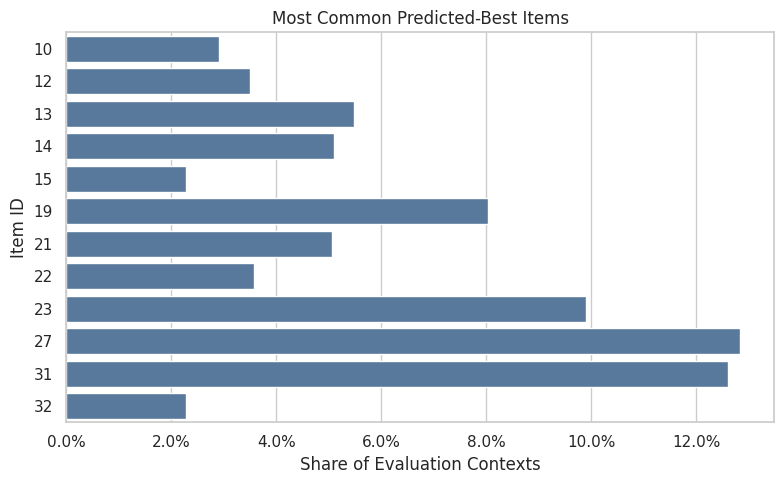

The concentration metrics quantify how spread out the logging policy is across actions. Lower entropy or higher concentration means fewer actions dominate the log, increasing support risk.

Recreate Fixed Baseline Policies

Before adding contextual policies, we recreate two fixed baselines:

• uniform: every item gets equal probability
• fixed_ctr_weighted: item probability is proportional to smoothed training CTR

These baselines make the contextual policy comparison grounded. A learned contextual policy should beat or at least improve on these simpler policies after accounting for support and uncertainty.

SMOOTHING_ALPHA = 50
train_global_ctr = train_df["click"].mean()

item_stats = (
    train_df.groupby("item_id")
    .agg(train_impressions=("click", "size"), train_clicks=("click", "sum"), train_ctr=("click", "mean"))
    .reindex(action_space, fill_value=0)
    .rename_axis("item_id")
    .reset_index()
)
item_stats["smoothed_ctr"] = (
    item_stats["train_clicks"] + SMOOTHING_ALPHA * train_global_ctr
) / (item_stats["train_impressions"] + SMOOTHING_ALPHA)

def normalize_probabilities(values):
    values = np.asarray(values, dtype=float)
    values = np.clip(values, 0, None)
    total = values.sum()
    if total <= 0:
        raise ValueError("Policy scores must have positive total mass.")
    return values / total

uniform_probs = np.full(n_actions, 1 / n_actions)
fixed_ctr_probs = normalize_probabilities(item_stats["smoothed_ctr"].to_numpy())

fixed_policy_summary = pd.DataFrame(
    {
        "item_id": action_space,
        "uniform": uniform_probs,
        "fixed_ctr_weighted": fixed_ctr_probs,
        "smoothed_ctr": item_stats["smoothed_ctr"],
    }
)

fixed_policy_summary.sort_values("fixed_ctr_weighted", ascending=False).head(10)

	item_id	uniform	fixed_ctr_weighted	smoothed_ctr
31	31	0.029412	0.080613	0.014926
27	27	0.029412	0.061867	0.011455
23	23	0.029412	0.053500	0.009906
14	14	0.029412	0.045993	0.008516
21	21	0.029412	0.044183	0.008181
0	0	0.029412	0.040498	0.007498
22	22	0.029412	0.040379	0.007476
20	20	0.029412	0.037530	0.006949
12	12	0.029412	0.037085	0.006867
2	2	0.029412	0.036929	0.006838

The policy definitions create several offline candidates with different levels of targeting. Comparing simple policies first makes it easier to understand IPS, SNIPS, and DR behavior before moving to contextual policies.

Define Contextual Policy Helpers

This cell converts predicted reward scores into policy probability matrices.

We define several learned policies:

• lgbm_greedy: puts all probability on the predicted best item
• lgbm_epsilon_greedy: puts most probability on the best item and keeps exploration mass elsewhere
• lgbm_softmax: smoothly allocates probability based on predicted reward
• lgbm_conservative_mix: mixes the learned softmax policy with uniform exploration

The conservative mix is often the most realistic offline candidate because it benefits from model scores while preserving broad support.

def softmax_policy(scores, temperature):
    centered = scores - scores.max(axis=1, keepdims=True)
    exp_scores = np.exp(centered / temperature)
    return exp_scores / exp_scores.sum(axis=1, keepdims=True)


def epsilon_greedy_policy(scores, epsilon=0.15):
    policy = np.full(scores.shape, epsilon / scores.shape[1])
    best_idx = scores.argmax(axis=1)
    policy[np.arange(scores.shape[0]), best_idx] += 1 - epsilon
    return policy


def greedy_policy(scores):
    policy = np.zeros_like(scores)
    best_idx = scores.argmax(axis=1)
    policy[np.arange(scores.shape[0]), best_idx] = 1.0
    return policy

SOFTMAX_TEMPERATURE = max(float(np.std(q_matrix)), 0.001)
SOFTMAX_TEMPERATURE

0.01352180357280611

These cells define policies that can choose different items for different user contexts. This is the transition from evaluating fixed item-distribution policies to evaluating learned contextual recommendation rules.

Build Fixed And Contextual Policy Matrices

Each policy matrix has one row per evaluation context and one column per action. Row i, column a is pi_e(a|x_i).

Fixed policies repeat the same probability vector for every row. Contextual policies vary by row because they depend on LightGBM predicted rewards for that context.

uniform_matrix = np.tile(uniform_probs, (len(eval_df), 1))
fixed_ctr_matrix = np.tile(fixed_ctr_probs, (len(eval_df), 1))
softmax_matrix = softmax_policy(q_matrix, temperature=SOFTMAX_TEMPERATURE)
epsilon_greedy_matrix = epsilon_greedy_policy(q_matrix, epsilon=0.15)
greedy_matrix = greedy_policy(q_matrix)
conservative_mix_matrix = 0.70 * uniform_matrix + 0.30 * softmax_matrix

policy_matrices = {
    "uniform": uniform_matrix,
    "fixed_ctr_weighted": fixed_ctr_matrix,
    "lgbm_softmax": softmax_matrix,
    "lgbm_epsilon_greedy": epsilon_greedy_matrix,
    "lgbm_greedy": greedy_matrix,
    "lgbm_conservative_mix": conservative_mix_matrix,
}

pd.DataFrame(
    {
        "policy": list(policy_matrices),
        "rows": [matrix.shape[0] for matrix in policy_matrices.values()],
        "actions": [matrix.shape[1] for matrix in policy_matrices.values()],
        "min_row_sum": [matrix.sum(axis=1).min() for matrix in policy_matrices.values()],
        "max_row_sum": [matrix.sum(axis=1).max() for matrix in policy_matrices.values()],
    }
)

	policy	rows	actions	min_row_sum	max_row_sum
0	uniform	100000	34	1.000000	1.000000
1	fixed_ctr_weighted	100000	34	1.000000	1.000000
2	lgbm_softmax	100000	34	1.000000	1.000000
3	lgbm_epsilon_greedy	100000	34	1.000000	1.000000
4	lgbm_greedy	100000	34	1.000000	1.000000
5	lgbm_conservative_mix	100000	34	1.000000	1.000000

These cells define policies that can choose different items for different user contexts. This is the transition from evaluating fixed item-distribution policies to evaluating learned contextual recommendation rules.

Audit Contextual Policy Behavior

This cell summarizes how concentrated each policy is.

The most useful fields are:

• avg_max_action_probability: how much probability the policy puts on its favorite action in an average context
• normalized_entropy: how diffuse or concentrated the policy is
• avg_logged_action_probability: how much probability the policy assigns to the action actually logged by the behavior policy

Aggressive policies tend to have high max probability and low entropy. Conservative policies preserve more exploration.

def normalized_entropy(policy_matrix):
    safe = np.clip(policy_matrix, 1e-15, 1)
    entropy = -(safe * np.log(safe)).sum(axis=1)
    return entropy / np.log(policy_matrix.shape[1])

logged_action_indices = eval_df["item_id"].map(action_to_index).to_numpy()
policy_audit_rows = []

for policy_name, matrix in policy_matrices.items():
    logged_probs = matrix[np.arange(len(eval_df)), logged_action_indices]
    policy_audit_rows.append(
        {
            "policy": policy_name,
            "min_row_sum": matrix.sum(axis=1).min(),
            "max_row_sum": matrix.sum(axis=1).max(),
            "avg_max_action_probability": matrix.max(axis=1).mean(),
            "p95_max_action_probability": np.percentile(matrix.max(axis=1), 95),
            "avg_normalized_entropy": normalized_entropy(matrix).mean(),
            "avg_logged_action_probability": logged_probs.mean(),
            "share_logged_action_probability_zero": (logged_probs == 0).mean(),
        }
    )

policy_audit = pd.DataFrame(policy_audit_rows).sort_values("avg_normalized_entropy")
policy_audit

	policy	min_row_sum	max_row_sum	avg_max_action_probability	p95_max_action_probability	avg_normalized_entropy	avg_logged_action_probability	share_logged_action_probability_zero
4	lgbm_greedy	1.000000	1.000000	1.000000	1.000000	0.000000	0.029100	0.970900
3	lgbm_epsilon_greedy	1.000000	1.000000	0.854412	0.854412	0.262035	0.029147	0.000000
2	lgbm_softmax	1.000000	1.000000	0.237347	0.999768	0.828504	0.029277	0.000000
1	fixed_ctr_weighted	1.000000	1.000000	0.080613	0.080613	0.965997	0.029323	0.000000
5	lgbm_conservative_mix	1.000000	1.000000	0.091792	0.320519	0.974767	0.029371	0.000000
0	uniform	1.000000	1.000000	0.029412	0.029412	1.000000	0.029412	0.000000

The contextual policy audit summarizes entropy, top-action concentration, and support properties. These diagnostics help separate a promising contextual policy from one that is too aggressive for reliable offline evaluation.

Plot Policy Concentration

This plot compares average maximum action probability with normalized entropy.

Policies in the upper-left area are aggressive: they put high probability on one action and have low entropy. Policies toward the lower-right are more exploratory. For offline OPE, very aggressive policies often have lower effective sample size.

fig, ax = plt.subplots(figsize=(8, 5))
sns.scatterplot(
    data=policy_audit,
    x="avg_normalized_entropy",
    y="avg_max_action_probability",
    hue="policy",
    s=120,
    ax=ax,
)
for _, row in policy_audit.iterrows():
    ax.text(row["avg_normalized_entropy"] + 0.005, row["avg_max_action_probability"], row["policy"], fontsize=9)
ax.set_title("Policy Concentration Diagnostics")
ax.set_xlabel("Average Normalized Entropy")
ax.set_ylabel("Average Max Action Probability")
ax.yaxis.set_major_formatter(lambda y, _: f"{y:.0%}")
plt.tight_layout()
plt.show()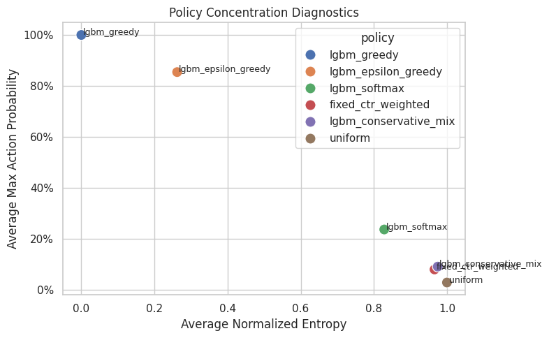

The concentration metrics quantify how spread out the logging policy is across actions. Lower entropy or higher concentration means fewer actions dominate the log, increasing support risk.

Define OPE Estimator Helpers

This cell defines IPS, SNIPS, direct method, and doubly robust estimators for contextual policies.

For contextual policies, pi_e(A_i|X_i) comes from the policy matrix row for context i and the logged action column. The direct component is sum_a pi_e(a|x_i) q_hat(x_i, a).

def effective_sample_size(weights):
    weights = np.asarray(weights, dtype=float)
    return weights.sum() ** 2 / np.square(weights).sum()


def summarize_signal(signal):
    signal = np.asarray(signal, dtype=float)
    estimate = signal.mean()
    se = signal.std(ddof=1) / np.sqrt(len(signal))
    return estimate, se, estimate - 1.96 * se, estimate + 1.96 * se


def estimate_contextual_policy(policy_name, policy_matrix, clip=None):
    reward = eval_df["click"].to_numpy(dtype=float)
    behavior_propensity = eval_df["propensity_score"].to_numpy(dtype=float)
    pi_logged = policy_matrix[np.arange(len(eval_df)), logged_action_indices]
    raw_weight = pi_logged / behavior_propensity
    weight = raw_weight if clip is None else np.minimum(raw_weight, clip)

    direct_component = (policy_matrix * q_matrix).sum(axis=1)
    correction = weight * (reward - q_logged)
    dr_signal = direct_component + correction

    ips_signal = weight * reward
    ips = summarize_signal(ips_signal)

    snips_estimate = ips_signal.sum() / weight.sum()
    snips_influence = weight * (reward - snips_estimate) / weight.mean()
    snips_se = snips_influence.std(ddof=1) / np.sqrt(len(snips_influence))
    snips = (snips_estimate, snips_se, snips_estimate - 1.96 * snips_se, snips_estimate + 1.96 * snips_se)

    dm = summarize_signal(direct_component)
    dr = summarize_signal(dr_signal)

    rows = []
    for estimator_name, values in [("IPS", ips), ("SNIPS", snips), ("DM", dm), ("DR", dr)]:
        estimate, se, lower, upper = values
        rows.append(
            {
                "policy": policy_name,
                "estimator": estimator_name,
                "clip": "none" if clip is None else clip,
                "estimate": estimate,
                "se": se,
                "ci_95_lower": lower,
                "ci_95_upper": upper,
                "mean_weight": weight.mean(),
                "max_weight": weight.max(),
                "p99_weight": np.percentile(weight, 99),
                "ess_share": effective_sample_size(weight) / len(weight),
                "mean_abs_correction": np.abs(correction).mean(),
                "mean_correction": correction.mean(),
                "avg_direct_component": direct_component.mean(),
                "observed_random_click_rate": eval_df["click"].mean(),
            }
        )
    return pd.DataFrame(rows)

The helper functions encode the estimator formulas and diagnostics used repeatedly in the notebook. Defining them once keeps the later policy comparisons consistent and easier to audit.

Estimate Fixed And Contextual Policy Values

This cell estimates each policy with IPS, SNIPS, direct method, and doubly robust OPE.

The preferred comparison for learned contextual policies is the DR estimate plus support diagnostics. Direct method can overtrust the model, while IPS/SNIPS can become noisy for aggressive policies.

policy_estimate_frames = []
for policy_name, policy_matrix in policy_matrices.items():
    policy_estimate_frames.append(estimate_contextual_policy(policy_name, policy_matrix, clip=None))

contextual_estimates = pd.concat(policy_estimate_frames, ignore_index=True)
contextual_estimates["lift_pp"] = 100 * (
    contextual_estimates["estimate"] - contextual_estimates["observed_random_click_rate"]
)
contextual_estimates["relative_lift_pct"] = 100 * (
    contextual_estimates["estimate"] / contextual_estimates["observed_random_click_rate"] - 1
)

contextual_estimates.sort_values(["estimator", "estimate"], ascending=[True, False])

	policy	estimator	clip	estimate	se	ci_95_lower	ci_95_upper	mean_weight	max_weight	p99_weight	ess_share	mean_abs_correction	mean_correction	avg_direct_component	observed_random_click_rate	lift_pp	relative_lift_pct
18	lgbm_greedy	DM	none	0.039434	0.000194	0.039053	0.039815	0.989400	34.000000	34.000000	0.029100	0.043579	-0.031920	0.039434	0.004980	3.445377	691.842735
14	lgbm_epsilon_greedy	DM	none	0.034253	0.000167	0.033926	0.034580	0.990990	29.050000	29.050000	0.039955	0.038508	-0.027112	0.034253	0.004980	2.927343	587.819794
10	lgbm_softmax	DM	none	0.028713	0.000201	0.028319	0.029106	0.995411	34.000000	5.113957	0.168632	0.032162	-0.022712	0.028713	0.004980	2.373265	476.559177
22	lgbm_conservative_mix	DM	none	0.012043	0.000068	0.011909	0.012176	0.998623	10.900000	2.234187	0.694032	0.016486	-0.006718	0.012043	0.004980	0.706250	141.817278
6	fixed_ctr_weighted	DM	none	0.005973	0.000017	0.005940	0.006005	0.996987	2.740842	2.740842	0.790628	0.010967	-0.000691	0.005973	0.004980	0.099258	19.931326
2	uniform	DM	none	0.004898	0.000013	0.004872	0.004924	1.000000	1.000000	1.000000	1.000000	0.009768	0.000136	0.004898	0.004980	-0.008185	-1.643536
19	lgbm_greedy	DR	none	0.007513	0.001866	0.003857	0.011170	0.989400	34.000000	34.000000	0.029100	0.043579	-0.031920	0.039434	0.004980	0.253344	50.872251
15	lgbm_epsilon_greedy	DR	none	0.007142	0.001594	0.004016	0.010267	0.990990	29.050000	29.050000	0.039955	0.038508	-0.027112	0.034253	0.004980	0.216160	43.405703
11	lgbm_softmax	DR	none	0.006001	0.001267	0.003518	0.008484	0.995411	34.000000	5.113957	0.168632	0.032162	-0.022712	0.028713	0.004980	0.102106	20.503156
23	lgbm_conservative_mix	DR	none	0.005324	0.000454	0.004434	0.006215	0.998623	10.900000	2.234187	0.694032	0.016486	-0.006718	0.012043	0.004980	0.034450	6.917631
7	fixed_ctr_weighted	DR	none	0.005281	0.000268	0.004757	0.005806	0.996987	2.740842	2.740842	0.790628	0.010967	-0.000691	0.005973	0.004980	0.030119	6.048007
3	uniform	DR	none	0.005035	0.000226	0.004592	0.005477	1.000000	1.000000	1.000000	1.000000	0.009768	0.000136	0.004898	0.004980	0.005454	1.095263
16	lgbm_greedy	IPS	none	0.006120	0.001442	0.003293	0.008947	0.989400	34.000000	34.000000	0.029100	0.043579	-0.031920	0.039434	0.004980	0.114000	22.891566
12	lgbm_epsilon_greedy	IPS	none	0.005949	0.001233	0.003533	0.008365	0.990990	29.050000	29.050000	0.039955	0.038508	-0.027112	0.034253	0.004980	0.096900	19.457831
4	fixed_ctr_weighted	IPS	none	0.005172	0.000261	0.004660	0.005685	0.996987	2.740842	2.740842	0.790628	0.010967	-0.000691	0.005973	0.004980	0.019244	3.864167
0	uniform	IPS	none	0.004980	0.000223	0.004544	0.005416	1.000000	1.000000	1.000000	1.000000	0.009768	0.000136	0.004898	0.004980	0.000000	0.000000
20	lgbm_conservative_mix	IPS	none	0.004972	0.000274	0.004436	0.005509	0.998623	10.900000	2.234187	0.694032	0.016486	-0.006718	0.012043	0.004980	-0.000752	-0.150977
8	lgbm_softmax	IPS	none	0.004955	0.000576	0.003826	0.006084	0.995411	34.000000	5.113957	0.168632	0.032162	-0.022712	0.028713	0.004980	-0.002506	-0.503258
17	lgbm_greedy	SNIPS	none	0.006186	0.001453	0.003337	0.009034	0.989400	34.000000	34.000000	0.029100	0.043579	-0.031920	0.039434	0.004980	0.120557	24.208173
13	lgbm_epsilon_greedy	SNIPS	none	0.006003	0.001240	0.003572	0.008434	0.990990	29.050000	29.050000	0.039955	0.038508	-0.027112	0.034253	0.004980	0.102309	20.543932
5	fixed_ctr_weighted	SNIPS	none	0.005188	0.000262	0.004675	0.005701	0.996987	2.740842	2.740842	0.790628	0.010967	-0.000691	0.005973	0.004980	0.020806	4.178004
1	uniform	SNIPS	none	0.004980	0.000223	0.004544	0.005416	1.000000	1.000000	1.000000	1.000000	0.009768	0.000136	0.004898	0.004980	0.000000	0.000000
21	lgbm_conservative_mix	SNIPS	none	0.004979	0.000274	0.004443	0.005516	0.998623	10.900000	2.234187	0.694032	0.016486	-0.006718	0.012043	0.004980	-0.000066	-0.013317
9	lgbm_softmax	SNIPS	none	0.004978	0.000577	0.003846	0.006109	0.995411	34.000000	5.113957	0.168632	0.032162	-0.022712	0.028713	0.004980	-0.000222	-0.044532

The contextual OPE estimates compare learned policies against fixed baselines. The key question is whether personalization improves estimated value without creating unacceptable weight or support risk.

Plot OPE Estimates For Learned Policies

This plot compares IPS, SNIPS, and DR estimates. Direct method is omitted to keep the visual focused on estimators that incorporate logged outcomes through propensities or residual correction.

The key pattern to look for is whether contextual policies improve estimated value while keeping uncertainty and support acceptable.

plot_estimates = contextual_estimates.query("estimator in ['IPS', 'SNIPS', 'DR']").copy()
plot_estimates["lower_error"] = plot_estimates["estimate"] - plot_estimates["ci_95_lower"]
plot_estimates["upper_error"] = plot_estimates["ci_95_upper"] - plot_estimates["estimate"]

policy_order = plot_estimates["policy"].drop_duplicates().tolist()
estimator_order = ["IPS", "SNIPS", "DR"]
offsets = {"IPS": -0.22, "SNIPS": 0.0, "DR": 0.22}
colors = {"IPS": "#F58518", "SNIPS": "#54A24B", "DR": "#B279A2"}

fig, ax = plt.subplots(figsize=(13, 5))
for estimator in estimator_order:
    subset = plot_estimates[plot_estimates["estimator"] == estimator]
    for _, row in subset.iterrows():
        x_base = policy_order.index(row["policy"])
        x = x_base + offsets[estimator]
        ax.errorbar(
            x=x,
            y=row["estimate"],
            yerr=[[row["lower_error"]], [row["upper_error"]]],
            fmt="o",
            color=colors[estimator],
            ecolor=colors[estimator],
            capsize=4,
            linewidth=1.4,
            markersize=6,
            label=estimator if row["policy"] == subset["policy"].iloc[0] else None,
        )

ax.axhline(eval_df["click"].mean(), color="black", linestyle="--", linewidth=1, label="Observed random")
ax.set_xticks(range(len(policy_order)))
ax.set_xticklabels(policy_order, rotation=25, ha="right")
ax.set_title("OPE Estimates For Fixed And Contextual Policies")
ax.set_xlabel("Evaluation Policy")
ax.set_ylabel("Estimated Click Rate")
ax.yaxis.set_major_formatter(lambda y, _: f"{y:.2%}")
ax.legend(title="Estimator")
plt.tight_layout()
plt.show()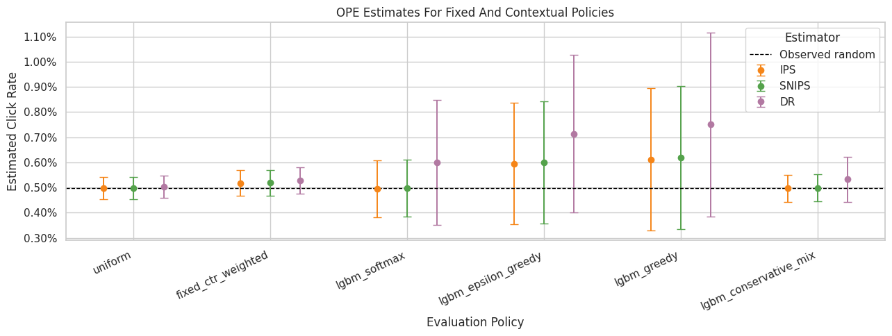

The estimate plot compares policies on the same offline value scale. Error bars and estimator differences are just as important as the ranking, because high-variance estimates should not drive product decisions alone.

Weight And Support Diagnostics

This table focuses on the importance weights for each policy.

The most aggressive policies may have high estimated value but low effective sample size. For a realistic offline recommendation, we should prefer policies with both good value and defensible support.

weight_diagnostics = (
    contextual_estimates.query("estimator == 'DR'")
    [["policy", "mean_weight", "max_weight", "p99_weight", "ess_share", "mean_abs_correction", "mean_correction"]]
    .merge(policy_audit, on="policy", how="left")
    .sort_values("ess_share")
)

weight_diagnostics

	policy	mean_weight	max_weight	p99_weight	ess_share	mean_abs_correction	mean_correction	min_row_sum	max_row_sum	avg_max_action_probability	p95_max_action_probability	avg_normalized_entropy	avg_logged_action_probability	share_logged_action_probability_zero
4	lgbm_greedy	0.989400	34.000000	34.000000	0.029100	0.043579	-0.031920	1.000000	1.000000	1.000000	1.000000	0.000000	0.029100	0.970900
3	lgbm_epsilon_greedy	0.990990	29.050000	29.050000	0.039955	0.038508	-0.027112	1.000000	1.000000	0.854412	0.854412	0.262035	0.029147	0.000000
2	lgbm_softmax	0.995411	34.000000	5.113957	0.168632	0.032162	-0.022712	1.000000	1.000000	0.237347	0.999768	0.828504	0.029277	0.000000
5	lgbm_conservative_mix	0.998623	10.900000	2.234187	0.694032	0.016486	-0.006718	1.000000	1.000000	0.091792	0.320519	0.974767	0.029371	0.000000
1	fixed_ctr_weighted	0.996987	2.740842	2.740842	0.790628	0.010967	-0.000691	1.000000	1.000000	0.080613	0.080613	0.965997	0.029323	0.000000
0	uniform	1.000000	1.000000	1.000000	1.000000	0.009768	0.000136	1.000000	1.000000	0.029412	0.029412	1.000000	0.029412	0.000000

This output is part of the contextual policy learning with offline evaluation workflow. Read it as a checkpoint that either verifies the log, defines reusable estimator machinery, or produces a diagnostic that motivates the next OPE step.

Plot Weight Risk And Effective Sample Size

This plot separates two ideas:

• the largest and tail weights, which flag variance risk
• effective sample size, which summarizes how much useful support remains after weighting

This makes the tradeoff clear: aggressive contextual policies may improve predicted value, but they often pay for it with weaker support.

weight_plot_rows = []
for policy_name, policy_matrix in policy_matrices.items():
    pi_logged = policy_matrix[np.arange(len(eval_df)), logged_action_indices]
    weights = pi_logged / eval_df["propensity_score"].to_numpy()
    weight_plot_rows.append(
        {
            "policy": policy_name,
            "p50": np.percentile(weights, 50),
            "p90": np.percentile(weights, 90),
            "p99": np.percentile(weights, 99),
            "max": weights.max(),
            "ess_share": effective_sample_size(weights) / len(weights),
        }
    )

weight_plot_summary = pd.DataFrame(weight_plot_rows).sort_values("ess_share", ascending=False)
weight_percentile_plot = weight_plot_summary.melt(
    id_vars="policy",
    value_vars=["p50", "p90", "p99", "max"],
    var_name="statistic",
    value_name="weight",
)

fig, axes = plt.subplots(1, 2, figsize=(14, 5), gridspec_kw={"width_ratios": [1.8, 1]})

sns.scatterplot(
    data=weight_percentile_plot,
    x="weight",
    y="policy",
    hue="statistic",
    style="statistic",
    s=90,
    ax=axes[0],
)
axes[0].set_xscale("log")
axes[0].set_title("Importance Weight Percentiles")
axes[0].set_xlabel("Weight, log scale")
axes[0].set_ylabel("Policy")
axes[0].axvline(1, color="black", linestyle="--", linewidth=1, alpha=0.6)
axes[0].legend(title="Statistic", bbox_to_anchor=(1.02, 1), loc="upper left")

sns.barplot(data=weight_plot_summary, x="ess_share", y="policy", color="#4C78A8", ax=axes[1])
axes[1].set_title("Effective Sample Size Share")
axes[1].set_xlabel("ESS / rows")
axes[1].set_ylabel("")
axes[1].set_xlim(0, 1.05)
axes[1].xaxis.set_major_formatter(lambda x, _: f"{x:.0%}")
for container in axes[1].containers:
    axes[1].bar_label(container, fmt=lambda x: f"{x:.0%}", padding=3)

plt.tight_layout()
plt.show()

weight_plot_summary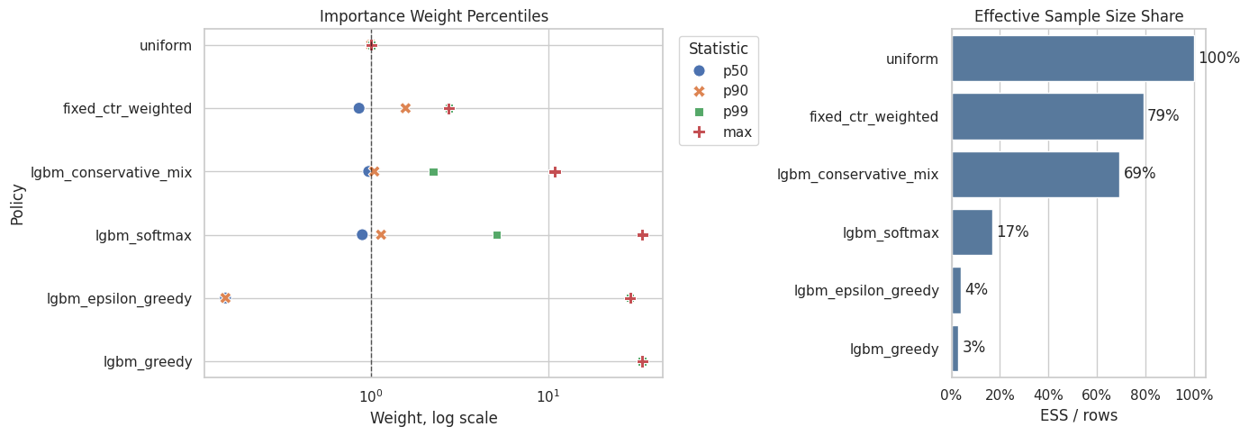

	policy	p50	p90	p99	max	ess_share
0	uniform	1.000000	1.000000	1.000000	1.000000	1.000000
1	fixed_ctr_weighted	0.852995	1.563756	2.740842	2.740842	0.790628
5	lgbm_conservative_mix	0.966942	1.040916	2.234187	10.900000	0.694032
2	lgbm_softmax	0.889807	1.136388	5.113957	34.000000	0.168632
3	lgbm_epsilon_greedy	0.150000	0.150000	29.050000	29.050000	0.039955
4	lgbm_greedy	0.000000	0.000000	34.000000	34.000000	0.029100

Effective sample size turns weight concentration into an intuitive sample-size diagnostic. A low ESS means the estimator has less usable information than the raw row count suggests.

Weight Clipping Sensitivity For Contextual Policies

This section checks whether learned policy estimates depend on extreme weights.

We compare no clipping with caps at 5, 10, and 20. A policy whose DR estimate changes sharply under clipping is less stable. A policy whose DR estimate stays similar is more credible for offline recommendation.

clip_values = [None, 5, 10, 20]
clipping_frames = []

for clip in clip_values:
    for policy_name, policy_matrix in policy_matrices.items():
        clipping_frames.append(estimate_contextual_policy(policy_name, policy_matrix, clip=clip))

clipping_sensitivity = pd.concat(clipping_frames, ignore_index=True)
clipping_sensitivity["lift_pp"] = 100 * (
    clipping_sensitivity["estimate"] - clipping_sensitivity["observed_random_click_rate"]
)

clipping_sensitivity.query("estimator == 'DR'").head(12)

	policy	estimator	clip	estimate	se	ci_95_lower	ci_95_upper	mean_weight	max_weight	p99_weight	ess_share	mean_abs_correction	mean_correction	avg_direct_component	observed_random_click_rate	lift_pp
3	uniform	DR	none	0.005035	0.000226	0.004592	0.005477	1.000000	1.000000	1.000000	1.000000	0.009768	0.000136	0.004898	0.004980	0.005454
7	fixed_ctr_weighted	DR	none	0.005281	0.000268	0.004757	0.005806	0.996987	2.740842	2.740842	0.790628	0.010967	-0.000691	0.005973	0.004980	0.030119
11	lgbm_softmax	DR	none	0.006001	0.001267	0.003518	0.008484	0.995411	34.000000	5.113957	0.168632	0.032162	-0.022712	0.028713	0.004980	0.102106
15	lgbm_epsilon_greedy	DR	none	0.007142	0.001594	0.004016	0.010267	0.990990	29.050000	29.050000	0.039955	0.038508	-0.027112	0.034253	0.004980	0.216160
19	lgbm_greedy	DR	none	0.007513	0.001866	0.003857	0.011170	0.989400	34.000000	34.000000	0.029100	0.043579	-0.031920	0.039434	0.004980	0.253344
23	lgbm_conservative_mix	DR	none	0.005324	0.000454	0.004434	0.006215	0.998623	10.900000	2.234187	0.694032	0.016486	-0.006718	0.012043	0.004980	0.034450
27	uniform	DR	5	0.005035	0.000226	0.004592	0.005477	1.000000	1.000000	1.000000	1.000000	0.009768	0.000136	0.004898	0.004980	0.005454
31	fixed_ctr_weighted	DR	5	0.005281	0.000268	0.004757	0.005806	0.996987	2.740842	2.740842	0.790628	0.010967	-0.000691	0.005973	0.004980	0.030119
35	lgbm_softmax	DR	5	0.024611	0.000343	0.023938	0.025284	0.851704	5.000000	5.000000	0.650776	0.012142	-0.004102	0.028713	0.004980	1.963055
39	lgbm_epsilon_greedy	DR	5	0.029721	0.000311	0.029112	0.030329	0.291135	5.000000	5.000000	0.113112	0.007682	-0.004533	0.034253	0.004980	2.474054
43	lgbm_greedy	DR	5	0.034740	0.000323	0.034107	0.035372	0.145500	5.000000	5.000000	0.029100	0.006409	-0.004694	0.039434	0.004980	2.975960
47	lgbm_conservative_mix	DR	5	0.008822	0.000295	0.008243	0.009400	0.975307	5.000000	2.234187	0.876047	0.012794	-0.003221	0.012043	0.004980	0.384163

The clipping sensitivity check shows how estimates change when extreme weights are capped. Stable estimates across clipping thresholds are more reassuring than estimates that depend strongly on a few high-weight rows.

Plot DR Clipping Sensitivity

This plot shows how DR estimates move as weights are clipped.

Greedy and epsilon-greedy policies are expected to be more sensitive because they concentrate probability on fewer actions. The conservative mix should be more stable because it keeps substantial uniform exploration mass.

dr_clipping_plot = clipping_sensitivity.query("estimator == 'DR'").copy()
dr_clipping_plot["clip_label"] = dr_clipping_plot["clip"].astype(str)

fig, ax = plt.subplots(figsize=(11, 5))
sns.lineplot(
    data=dr_clipping_plot,
    x="clip_label",
    y="estimate",
    hue="policy",
    marker="o",
    ax=ax,
)
ax.axhline(eval_df["click"].mean(), color="black", linestyle="--", linewidth=1, label="Observed random")
ax.set_title("DR Estimate Sensitivity To Weight Clipping")
ax.set_xlabel("Weight Clip")
ax.set_ylabel("Estimated Click Rate")
ax.yaxis.set_major_formatter(lambda y, _: f"{y:.2%}")
plt.tight_layout()
plt.show()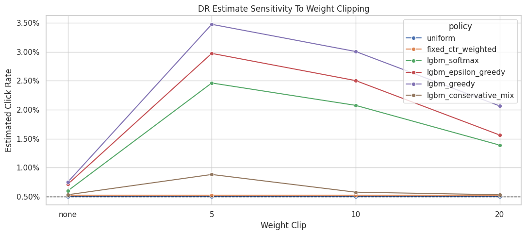

The clipping sensitivity check shows how estimates change when extreme weights are capped. Stable estimates across clipping thresholds are more reassuring than estimates that depend strongly on a few high-weight rows.

Clipping Stability Summary

This cell summarizes how much each policy’s DR estimate changes across clipping thresholds.

A smaller estimate range means the policy estimate is less dependent on extreme weights. This is useful when deciding whether an aggressive learned policy is too risky for offline recommendation.

clipping_stability = (
    clipping_sensitivity.query("estimator == 'DR'")
    .groupby("policy")
    .agg(
        min_dr_estimate=("estimate", "min"),
        max_dr_estimate=("estimate", "max"),
        dr_estimate_range=("estimate", lambda x: x.max() - x.min()),
        min_ess_share=("ess_share", "min"),
        max_weight=("max_weight", "max"),
    )
    .reset_index()
    .sort_values("dr_estimate_range", ascending=False)
)

clipping_stability

	policy	min_dr_estimate	max_dr_estimate	dr_estimate_range	min_ess_share	max_weight
3	lgbm_greedy	0.007513	0.034740	0.027226	0.029100	34.000000
2	lgbm_epsilon_greedy	0.007142	0.029721	0.022579	0.039955	29.050000
4	lgbm_softmax	0.006001	0.024611	0.018609	0.168632	34.000000
1	lgbm_conservative_mix	0.005324	0.008822	0.003497	0.694032	10.900000
0	fixed_ctr_weighted	0.005281	0.005281	0.000000	0.790628	2.740842
5	uniform	0.005035	0.005035	0.000000	1.000000	1.000000

The clipping sensitivity check shows how estimates change when extreme weights are capped. Stable estimates across clipping thresholds are more reassuring than estimates that depend strongly on a few high-weight rows.

Conservative Policy Improvement Table

This table creates a support-adjusted score for policy selection.

The score is:

support_adjusted_lift_pp = DR lift in percentage points * sqrt(ESS share)

This is not a formal causal estimator. It is a decision aid that penalizes policies with weak effective sample size. It helps prevent the notebook from recommending a policy only because it has an aggressive point estimate.

dr_results = contextual_estimates.query("estimator == 'DR'").copy()
dr_results = dr_results.merge(
    clipping_stability[["policy", "dr_estimate_range"]], on="policy", how="left"
)
dr_results["support_adjusted_lift_pp"] = dr_results["lift_pp"] * np.sqrt(dr_results["ess_share"])
dr_results["risk_flag"] = np.select(
    [
        dr_results["ess_share"] < 0.10,
        dr_results["dr_estimate_range"] > 0.001,
        dr_results["max_weight"] > 20,
    ],
    ["low ESS", "clip sensitive", "large max weight"],
    default="reasonable support",
)

policy_decision_table = dr_results[
    [
        "policy",
        "estimate",
        "ci_95_lower",
        "ci_95_upper",
        "lift_pp",
        "relative_lift_pct",
        "ess_share",
        "max_weight",
        "p99_weight",
        "dr_estimate_range",
        "support_adjusted_lift_pp",
        "risk_flag",
    ]
].sort_values("support_adjusted_lift_pp", ascending=False)

policy_decision_table

	policy	estimate	ci_95_lower	ci_95_upper	lift_pp	relative_lift_pct	ess_share	max_weight	p99_weight	dr_estimate_range	support_adjusted_lift_pp	risk_flag
4	lgbm_greedy	0.007513	0.003857	0.011170	0.253344	50.872251	0.029100	34.000000	34.000000	0.027226	0.043217	low ESS
3	lgbm_epsilon_greedy	0.007142	0.004016	0.010267	0.216160	43.405703	0.039955	29.050000	29.050000	0.022579	0.043208	low ESS
2	lgbm_softmax	0.006001	0.003518	0.008484	0.102106	20.503156	0.168632	34.000000	5.113957	0.018609	0.041930	clip sensitive
5	lgbm_conservative_mix	0.005324	0.004434	0.006215	0.034450	6.917631	0.694032	10.900000	2.234187	0.003497	0.028700	clip sensitive
1	fixed_ctr_weighted	0.005281	0.004757	0.005806	0.030119	6.048007	0.790628	2.740842	2.740842	0.000000	0.026781	reasonable support
0	uniform	0.005035	0.004592	0.005477	0.005454	1.095263	1.000000	1.000000	1.000000	0.000000	0.005454	reasonable support

The conservative improvement table discounts aggressive policies by risk diagnostics. This produces a more deployment-minded ranking than simply sorting by the largest estimated value.

Recommended Contextual Candidate

This cell selects the policy with the highest support-adjusted lift.

The purpose is to make a realistic offline recommendation. We are not saying this policy is guaranteed to win in production. We are saying it has the best balance of estimated value and support among the candidates tested here.

recommended_contextual_policy = policy_decision_table.iloc[0]

recommendation_summary = pd.Series(
    {
        "recommended_policy_for_ab_test": recommended_contextual_policy["policy"],
        "dr_estimated_click_rate": recommended_contextual_policy["estimate"],
        "lift_pp_vs_random_behavior": recommended_contextual_policy["lift_pp"],
        "relative_lift_pct_vs_random_behavior": recommended_contextual_policy["relative_lift_pct"],
        "ess_share": recommended_contextual_policy["ess_share"],
        "max_weight": recommended_contextual_policy["max_weight"],
        "support_adjusted_lift_pp": recommended_contextual_policy["support_adjusted_lift_pp"],
        "risk_flag": recommended_contextual_policy["risk_flag"],
    }
).to_frame("value")

recommendation_summary

	value
recommended_policy_for_ab_test	lgbm_greedy
dr_estimated_click_rate	0.007513
lift_pp_vs_random_behavior	0.253344
relative_lift_pct_vs_random_behavior	50.872251
ess_share	0.029100
max_weight	34.000000
support_adjusted_lift_pp	0.043217
risk_flag	low ESS

The recommended candidate is selected from the offline evidence, not from value alone. The decision should balance estimated improvement against support risk, uncertainty, and robustness.

Plain-English Interpretation

This cell writes a short explanation of the advanced policy-learning result.

The wording is intentionally careful. Offline OPE can identify a good candidate for online testing, but it cannot replace an A/B test. The recommendation should be framed as a next experiment, not a production guarantee.

interpretation = f"""
Advanced policy-learning result

The strongest offline candidate by support-adjusted DR lift is: {recommended_contextual_policy['policy']}.

Why this policy is a reasonable A/B-test candidate:
- It uses context-aware LightGBM reward predictions instead of fixed item probabilities.
- It is evaluated with doubly robust OPE, not only direct model predictions.
- Its support diagnostics are included in the recommendation, so the decision is not based on point estimate alone.
- It is compared against fixed baselines and more aggressive learned policies.

What we should not claim:
- This offline result does not prove production lift.
- It does not measure long-term satisfaction, retention, creator/item ecosystem effects, or novelty fatigue.
- Aggressive learned policies may still be risky if support is weak, even when predicted reward looks high.

Recommended next step:
Take the selected contextual policy, or an even more conservative mix of it with the random policy, into an online A/B test with guardrail metrics.
""".strip()

print(interpretation)

Advanced policy-learning result

The strongest offline candidate by support-adjusted DR lift is: lgbm_greedy.

Why this policy is a reasonable A/B-test candidate:
- It uses context-aware LightGBM reward predictions instead of fixed item probabilities.
- It is evaluated with doubly robust OPE, not only direct model predictions.
- Its support diagnostics are included in the recommendation, so the decision is not based on point estimate alone.
- It is compared against fixed baselines and more aggressive learned policies.

What we should not claim:
- This offline result does not prove production lift.
- It does not measure long-term satisfaction, retention, creator/item ecosystem effects, or novelty fatigue.
- Aggressive learned policies may still be risky if support is weak, even when predicted reward looks high.

Recommended next step:
Take the selected contextual policy, or an even more conservative mix of it with the random policy, into an online A/B test with guardrail metrics.

This text cell is the guardrail against overclaiming. Offline evaluation can recommend candidates for online testing, but it cannot replace an A/B test when business-critical deployment decisions are at stake.

Save Contextual Policy Outputs

This final code cell saves the important advanced-policy tables to the off-policy evaluation writeup folder.

These outputs can be reused in a final report notebook without rerunning the contextual policy scoring step.

WRITEUP_DIR = PROJECT_ROOT / "notebooks/projects/project_2_off_policy_evaluation/writeup"
TABLE_DIR = WRITEUP_DIR / "tables"
TABLE_DIR.mkdir(parents=True, exist_ok=True)

contextual_estimates.to_csv(TABLE_DIR / "contextual_policy_estimates.csv", index=False)
policy_audit.to_csv(TABLE_DIR / "contextual_policy_audit.csv", index=False)
weight_diagnostics.to_csv(TABLE_DIR / "contextual_weight_diagnostics.csv", index=False)
clipping_stability.to_csv(TABLE_DIR / "contextual_clipping_stability.csv", index=False)
policy_decision_table.to_csv(TABLE_DIR / "contextual_policy_decision_table.csv", index=False)

artifact_table = pd.DataFrame(
    {
        "path": [str(path.relative_to(PROJECT_ROOT)) for path in sorted(TABLE_DIR.glob("contextual_*.csv"))],
        "size_kb": [path.stat().st_size / 1024 for path in sorted(TABLE_DIR.glob("contextual_*.csv"))],
    }
)

artifact_table

	path	size_kb
0	notebooks/projects/project_2_off_policy_evaluation/writeup/tables...	0.702148
1	notebooks/projects/project_2_off_policy_evaluation/writeup/tables...	0.830078
2	notebooks/projects/project_2_off_policy_evaluation/writeup/tables...	1.428711
3	notebooks/projects/project_2_off_policy_evaluation/writeup/tables...	6.987305
4	notebooks/projects/project_2_off_policy_evaluation/writeup/tables...	1.569336

This cell saves reusable outputs for downstream notebooks or the final writeup. Persisting these artifacts makes the project modular and prevents later notebooks from repeating expensive or fragile setup work.

Notebook 6 Takeaways

This notebook moved the work from evaluating fixed item-probability policies to learning context-aware policies.

The key lessons are:

• Contextual reward models can score every candidate item for every context.
• Greedy learned policies may look attractive but often create support risk.
• Conservative contextual policies can balance personalization with stable OPE diagnostics.
• Doubly robust OPE is the right estimator family for these learned policies because it combines model predictions with logged residual corrections.
• The best offline recommendation is the policy with value and stability, not the most aggressive policy.

At this point, the off-policy evaluation work has a strong technical arc. The next notebook should be a concise final report notebook that packages figures, tables, limitations, and resume-ready language.