05 Policy Comparison And Sensitivity

This notebook is the final technical notebook for Off-Policy Evaluation of Recommendation Systems.

Notebook 3 introduced IPS and SNIPS. Notebook 4 added direct method and doubly robust OPE. Those estimates are useful, but a good offline policy recommendation should not depend on one exact modeling choice.

This notebook asks the decision-quality question:

Are the policy conclusions stable enough to recommend a policy for online A/B testing?

We stress-test the conclusions across three dimensions:

• weight clipping sensitivity: do estimates change when extreme weights are capped?
• reward model sensitivity: do DR estimates agree across logistic regression and LightGBM?
• time split sensitivity: does the same policy look good across different train/evaluation windows?

The goal is not to claim that offline OPE proves a production winner. The goal is to identify the most credible candidate for online experimentation and document the remaining risks.

Project Recap

The causal setup is a logged contextual bandit problem.

For each recommendation event, we observe context X, logged action A, reward Y, and behavior-policy propensity pi_b(A|X). We define candidate evaluation policies pi_e and estimate their values offline.

The estimators so far are:

• IPS: averages pi_e / pi_b * Y
• SNIPS: normalizes IPS weights by total weight
• Direct Method: averages reward model predictions under each policy
• Doubly Robust: direct method plus an importance-weighted residual correction

This notebook compares those estimators through the lens of stability. A policy with a slightly lower estimate but much stronger support may be a better A/B-test candidate than a policy with a high but fragile offline estimate.

Notebook Setup

This cell imports the libraries needed for sensitivity analysis. It also suppresses one known LightGBM/sklearn feature-name metadata warning so repeated model scoring does not clutter the notebook output.

The notebook uses the same modeling stack as Notebook 4: logistic regression and LightGBM reward models. We keep implementation explicit rather than relying on an OPE package so every estimate can be traced back to the formula.

from pathlib import Path
import warnings

import lightgbm as lgb
import matplotlib.pyplot as plt
import numpy as np
import pandas as pd
import seaborn as sns
from sklearn.compose import ColumnTransformer
from sklearn.linear_model import LogisticRegression
from sklearn.metrics import average_precision_score, brier_score_loss, log_loss, roc_auc_score
from sklearn.pipeline import Pipeline
from sklearn.preprocessing import OneHotEncoder, StandardScaler

pd.set_option("display.max_columns", 140)
pd.set_option("display.max_rows", 140)
pd.set_option("display.float_format", "{:.6f}".format)

sns.set_theme(style="whitegrid", context="notebook")

warnings.filterwarnings(
    "ignore",
    message="X does not have valid feature names, but LGBMClassifier was fitted with feature names",
    category=UserWarning,
)

This cell prepares the notebook environment for policy comparison and sensitivity analysis. There is no estimator output yet; the main value is that the imports, display settings, and plotting defaults are ready for the OPE diagnostics that follow.

Load The Random Open Bandit Sample

This cell loads the cached random/men sample used throughout the off-policy evaluation notebooks.

We keep the random log as the primary source for policy comparison because earlier notebooks showed that it has broad action support and stable logged propensities. That makes it the cleanest log for comparing evaluation policies.

RANDOM_SAMPLE_RELATIVE_PATH = Path("data/processed/open_bandit_random_men_sample.parquet")
PROJECT_ROOT = next(
    path
    for path in [Path.cwd(), *Path.cwd().parents]
    if (path / RANDOM_SAMPLE_RELATIVE_PATH).exists()
)

RANDOM_SAMPLE_PATH = PROJECT_ROOT / RANDOM_SAMPLE_RELATIVE_PATH
random_df = pd.read_parquet(RANDOM_SAMPLE_PATH).sort_values("timestamp").reset_index(drop=True)

pd.Series(
    {
        "project_root": PROJECT_ROOT,
        "random_sample_path": RANDOM_SAMPLE_PATH,
        "rows": len(random_df),
        "columns": random_df.shape[1],
        "observed_click_rate": random_df["click"].mean(),
    }
).to_frame("value")

	value
project_root	/home/apex/Documents/ranking_sys
random_sample_path	/home/apex/Documents/ranking_sys/data/processe...
rows	200000
columns	50
observed_click_rate	0.005190

The loaded table shape and preview confirm that the expected cached data is available. This check matters because all later OPE estimates depend on using the correct logged actions, rewards, contexts, and behavior propensities.

Define Shared Feature Groups

This cell defines the action space and reward-model feature groups.

The reward model features mirror Notebook 4. The most important engineered feature is selected_affinity, which selects the user-item affinity column corresponding to the candidate item being scored. This lets the same feature function work for logged actions and counterfactual candidate actions.

action_space = np.array(sorted(random_df["item_id"].unique()))
n_actions = len(action_space)

user_feature_cols = [col for col in random_df.columns if col.startswith("user_feature_")]
affinity_cols_by_action = [f"user-item_affinity_{item_id}" for item_id in action_space]
item_feature_cols = [col for col in random_df.columns if col.startswith("item_feature_")]

categorical_features = [
    "position",
    "hour",
    "item_id",
    *user_feature_cols,
    "item_feature_1",
    "item_feature_2",
    "item_feature_3",
]
numeric_features = ["selected_affinity", "item_feature_0"]
feature_cols = categorical_features + numeric_features

item_context = (
    random_df[["item_id", *item_feature_cols]]
    .drop_duplicates("item_id")
    .set_index("item_id")
    .sort_index()
)

pd.DataFrame(
    {
        "object": ["actions", "user features", "affinity columns", "item features", "model features"],
        "count": [n_actions, len(user_feature_cols), len(affinity_cols_by_action), len(item_feature_cols), len(feature_cols)],
    }
)

	object	count
0	actions	34
1	user features	4
2	affinity columns	34
3	item features	4
4	model features	12

These feature-building cells define the context used by reward models. Reward models need both user context and candidate item context so they can predict counterfactual rewards for actions that were not logged.

Define Reusable Feature Builders

This cell defines helper functions for reward-model feature construction.

make_logged_feature_frame creates features for the action that was actually logged. make_candidate_feature_frame creates features for every candidate action in each context row. The second function is what makes direct method and doubly robust OPE possible: it lets the reward model predict outcomes for actions we did not observe in that row.

def make_logged_feature_frame(df):
    """Create reward-model features for each row's logged action."""
    frame = df.copy()
    affinity_matrix = frame[affinity_cols_by_action].to_numpy()
    item_positions = frame["item_id"].map({item_id: idx for idx, item_id in enumerate(action_space)}).to_numpy()
    frame["selected_affinity"] = affinity_matrix[np.arange(len(frame)), item_positions]
    return frame[feature_cols]


def make_candidate_feature_frame(context_df):
    """Create reward-model features for every candidate action in each context row."""
    n_contexts = len(context_df)
    tiled_actions = np.tile(action_space, n_contexts)

    frame = pd.DataFrame(
        {
            "position": np.repeat(context_df["position"].to_numpy(), n_actions),
            "hour": np.repeat(context_df["hour"].to_numpy(), n_actions),
            "item_id": tiled_actions,
        }
    )

    for col in user_feature_cols:
        frame[col] = np.repeat(context_df[col].to_numpy(), n_actions)

    affinity_matrix = context_df[affinity_cols_by_action].to_numpy()
    frame["selected_affinity"] = affinity_matrix.reshape(-1)

    repeated_item_context = item_context.loc[tiled_actions, item_feature_cols].reset_index(drop=True)
    frame = pd.concat([frame, repeated_item_context], axis=1)

    return frame[feature_cols]

make_logged_feature_frame(random_df.head(3))

	position	hour	item_id	user_feature_0	user_feature_1	user_feature_2	user_feature_3	item_feature_1	item_feature_2	item_feature_3	selected_affinity	item_feature_0
0	1	0	0	cef3390ed299c09874189c387777674a	03a5648a76832f83c859d46bc06cb64a	2723d2eb8bba04e0362098011fa3997b	c39b0c7dd5d4eb9a18e7db6ba2f258f8	ce58bf66d7e62186e6ce01bafeea9d39	7c5498711d69681385d21c0e26923e7e	bbf748c6c978938bc63d432efa60191c	0.000000	-0.677183
1	3	0	25	cef3390ed299c09874189c387777674a	03a5648a76832f83c859d46bc06cb64a	2723d2eb8bba04e0362098011fa3997b	c39b0c7dd5d4eb9a18e7db6ba2f258f8	9874ffb54e9b0a269e29bbb2f5328735	7c5498711d69681385d21c0e26923e7e	bbf748c6c978938bc63d432efa60191c	0.000000	-0.461600
2	2	0	23	cef3390ed299c09874189c387777674a	03a5648a76832f83c859d46bc06cb64a	2723d2eb8bba04e0362098011fa3997b	c39b0c7dd5d4eb9a18e7db6ba2f258f8	55fe518d85813954c7d9b8a875ff2453	cc75031396a5aa830885915aa93f49d0	b61cfaadd526b816e3aeb9b7be4b4759	0.000000	-0.569392

These feature-building cells define the context used by reward models. Reward models need both user context and candidate item context so they can predict counterfactual rewards for actions that were not logged.

Define Evaluation Policy Builder

This helper recreates the candidate policies from Notebooks 3 and 4 using only the training split.

The candidate policies are intentionally simple:

• uniform: equal probability across items
• exposure_popularity: probability proportional to training exposure
• ctr_weighted: probability proportional to smoothed training CTR
• epsilon_greedy_top_ctr: most probability on the top smoothed-CTR item, with exploration mass elsewhere

Using the same policies keeps the notebook sequence coherent and lets us focus on sensitivity, not policy invention.

def normalize_probabilities(values):
    values = np.asarray(values, dtype=float)
    values = np.clip(values, 0, None)
    total = values.sum()
    if total <= 0:
        raise ValueError("Policy scores must have positive total mass.")
    return values / total


def build_policy_probabilities(train_df, smoothing_alpha=50, epsilon=0.15):
    train_global_ctr = train_df["click"].mean()
    item_stats = (
        train_df.groupby("item_id")
        .agg(train_impressions=("click", "size"), train_clicks=("click", "sum"), train_ctr=("click", "mean"))
        .reindex(action_space, fill_value=0)
        .rename_axis("item_id")
        .reset_index()
    )
    item_stats["smoothed_ctr"] = (
        item_stats["train_clicks"] + smoothing_alpha * train_global_ctr
    ) / (item_stats["train_impressions"] + smoothing_alpha)
    item_stats["train_exposure_share"] = item_stats["train_impressions"] / item_stats["train_impressions"].sum()

    uniform_probs = np.full(n_actions, 1 / n_actions)
    exposure_popularity_probs = normalize_probabilities(item_stats["train_exposure_share"].to_numpy())
    ctr_weighted_probs = normalize_probabilities(item_stats["smoothed_ctr"].to_numpy())

    epsilon_greedy_probs = np.full(n_actions, epsilon / n_actions)
    top_ctr_index = int(item_stats["smoothed_ctr"].to_numpy().argmax())
    epsilon_greedy_probs[top_ctr_index] += 1 - epsilon

    policy_probability_df = pd.DataFrame(
        {
            "item_id": action_space,
            "uniform": uniform_probs,
            "exposure_popularity": exposure_popularity_probs,
            "ctr_weighted": ctr_weighted_probs,
            "epsilon_greedy_top_ctr": epsilon_greedy_probs,
        }
    )
    return item_stats, policy_probability_df

The policy definitions create several offline candidates with different levels of targeting. Comparing simple policies first makes it easier to understand IPS, SNIPS, and DR behavior before moving to contextual policies.

Define Reward Model Builders

This helper returns a fresh reward-model pipeline for each sensitivity run.

A fresh pipeline matters because each split should be independent. Reusing fitted preprocessors or fitted models across splits would leak information and make the sensitivity analysis less trustworthy.

def build_preprocessor():
    return ColumnTransformer(
        transformers=[
            ("categorical", OneHotEncoder(handle_unknown="ignore"), categorical_features),
            ("numeric", StandardScaler(), numeric_features),
        ],
        remainder="drop",
    )


def build_reward_model(model_name):
    if model_name == "logistic":
        model = LogisticRegression(max_iter=500, solver="lbfgs")
    elif model_name == "lightgbm":
        model = lgb.LGBMClassifier(
            n_estimators=180,
            learning_rate=0.05,
            num_leaves=31,
            min_child_samples=100,
            subsample=0.85,
            colsample_bytree=0.85,
            random_state=42,
            verbose=-1,
        )
    elif model_name == "lightgbm_shallow":
        model = lgb.LGBMClassifier(
            n_estimators=120,
            learning_rate=0.06,
            num_leaves=15,
            min_child_samples=200,
            subsample=0.85,
            colsample_bytree=0.85,
            random_state=42,
            verbose=-1,
        )
    else:
        raise ValueError(f"Unknown reward model: {model_name}")

    return Pipeline(steps=[("preprocess", build_preprocessor()), ("model", model)])

The preprocessing and model-builder definitions make reward modeling reusable across policies, splits, and sensitivity checks. This helps ensure that estimator differences come from policy or model choices rather than inconsistent data preparation.

Define OPE Helper Functions

This cell defines the estimator machinery used throughout the notebook.

The helper functions compute effective sample size, large-sample confidence intervals, IPS, SNIPS, direct method, and doubly robust estimates. They also support weight clipping for sensitivity analysis. Clipping is applied to the importance-weighted terms, not to the direct-method prediction.

def effective_sample_size(weights):
    weights = np.asarray(weights, dtype=float)
    return weights.sum() ** 2 / np.square(weights).sum()


def summarize_signal(signal):
    signal = np.asarray(signal, dtype=float)
    estimate = signal.mean()
    se = signal.std(ddof=1) / np.sqrt(len(signal))
    return estimate, se, estimate - 1.96 * se, estimate + 1.96 * se


def estimate_policy_values(reward, weight, q_logged, direct_component, clip=None):
    reward = np.asarray(reward, dtype=float)
    raw_weight = np.asarray(weight, dtype=float)
    weight = raw_weight if clip is None else np.minimum(raw_weight, clip)
    q_logged = np.asarray(q_logged, dtype=float)
    direct_component = np.asarray(direct_component, dtype=float)

    ips_signal = weight * reward
    ips = summarize_signal(ips_signal)

    snips_estimate = ips_signal.sum() / weight.sum()
    snips_influence = weight * (reward - snips_estimate) / weight.mean()
    snips_se = snips_influence.std(ddof=1) / np.sqrt(len(snips_influence))
    snips = (snips_estimate, snips_se, snips_estimate - 1.96 * snips_se, snips_estimate + 1.96 * snips_se)

    dm = summarize_signal(direct_component)
    correction = weight * (reward - q_logged)
    dr_signal = direct_component + correction
    dr = summarize_signal(dr_signal)

    return {
        "IPS": ips,
        "SNIPS": snips,
        "DM": dm,
        "DR": dr,
        "ess_share": effective_sample_size(weight) / len(weight),
        "mean_weight": weight.mean(),
        "max_weight": weight.max(),
        "p99_weight": np.percentile(weight, 99),
        "mean_abs_correction": np.abs(correction).mean(),
        "mean_correction": correction.mean(),
    }

The helper functions encode the estimator formulas and diagnostics used repeatedly in the notebook. Defining them once keeps the later policy comparisons consistent and easier to audit.

Define Candidate-Action Scoring Helper

This helper computes direct-method components for every policy in batches.

For each evaluation context, it predicts q_hat(x, a) for all candidate actions. It then multiplies those predictions by each policy’s action probabilities. The output is one direct-method component per context and policy.

def compute_direct_components(model, contexts_df, policy_probability_df, batch_size=12_000):
    policy_cols = [col for col in policy_probability_df.columns if col != "item_id"]
    policy_probability_matrix = policy_probability_df[policy_cols].to_numpy()
    component_batches = []

    for start in range(0, len(contexts_df), batch_size):
        context_batch = contexts_df.iloc[start : start + batch_size]
        candidate_features = make_candidate_feature_frame(context_batch)
        q_hat = model.predict_proba(candidate_features)[:, 1].reshape(len(context_batch), n_actions)
        component_batches.append(q_hat @ policy_probability_matrix)

    components = np.vstack(component_batches)
    return pd.DataFrame(components, columns=policy_cols, index=contexts_df.index)

These cells score candidate actions under the reward model, which is what lets the direct method estimate values for policies that choose actions different from the logged one. This is the model-based complement to importance weighting.

Define One End-To-End Evaluation Function

This cell defines the core analysis function used by the sensitivity sections.

For a given train/evaluation split and reward model, it:

1. builds evaluation policies from the training split
2. trains a reward model on logged training rows
3. scores logged evaluation rows
4. scores all candidate actions for direct method
5. computes IPS, SNIPS, DM, and DR estimates
6. returns policy estimates, reward-model metrics, and policy probabilities

Having this in one function reduces copy-paste risk across the sensitivity analysis.

def run_ope_for_split(train_df, eval_df, model_name="lightgbm", split_name="main", clip=None):
    item_stats, policy_probability_df = build_policy_probabilities(train_df)
    policy_cols = [col for col in policy_probability_df.columns if col != "item_id"]

    X_train = make_logged_feature_frame(train_df)
    y_train = train_df["click"].astype(int)
    X_eval_logged = make_logged_feature_frame(eval_df)
    y_eval = eval_df["click"].astype(int)

    model = build_reward_model(model_name)
    model.fit(X_train, y_train)

    q_logged = model.predict_proba(X_eval_logged)[:, 1]
    direct_components = compute_direct_components(model, eval_df, policy_probability_df)

    model_metrics = {
        "split_name": split_name,
        "reward_model": model_name,
        "train_rows": len(train_df),
        "eval_rows": len(eval_df),
        "auc": roc_auc_score(y_eval, q_logged),
        "average_precision": average_precision_score(y_eval, q_logged),
        "log_loss": log_loss(y_eval, q_logged, labels=[0, 1]),
        "brier_score": brier_score_loss(y_eval, q_logged),
        "mean_prediction": q_logged.mean(),
        "observed_click_rate": y_eval.mean(),
    }

    eval_scored = eval_df[["timestamp", "item_id", "position", "click", "propensity_score"]].copy()
    result_rows = []
    reward = eval_scored["click"].to_numpy()

    for policy in policy_cols:
        probability_map = policy_probability_df.set_index("item_id")[policy]
        pi_e = eval_scored["item_id"].map(probability_map).to_numpy()
        weight = pi_e / eval_scored["propensity_score"].to_numpy()
        estimates = estimate_policy_values(
            reward=reward,
            weight=weight,
            q_logged=q_logged,
            direct_component=direct_components[policy].to_numpy(),
            clip=clip,
        )

        for estimator in ["IPS", "SNIPS", "DM", "DR"]:
            estimate, se, lower, upper = estimates[estimator]
            result_rows.append(
                {
                    "split_name": split_name,
                    "reward_model": model_name,
                    "policy": policy,
                    "estimator": estimator,
                    "clip": "none" if clip is None else clip,
                    "estimate": estimate,
                    "se": se,
                    "ci_95_lower": lower,
                    "ci_95_upper": upper,
                    "ess_share": estimates["ess_share"],
                    "mean_weight": estimates["mean_weight"],
                    "max_weight": estimates["max_weight"],
                    "p99_weight": estimates["p99_weight"],
                    "mean_abs_correction": estimates["mean_abs_correction"],
                    "mean_correction": estimates["mean_correction"],
                    "eval_observed_click_rate": y_eval.mean(),
                }
            )

    return pd.DataFrame(result_rows), pd.DataFrame([model_metrics]), policy_probability_df, item_stats

The end-to-end evaluation function packages splitting, reward modeling, policy scoring, and OPE estimation into one repeatable workflow. This makes sensitivity analysis possible without rewriting estimator logic each time.

Create The Main Split

This cell recreates the primary 50/50 time split from Notebooks 3 and 4.

The main split is used for detailed clipping and reward-model sensitivity. Later, split sensitivity uses several shorter evaluation windows to test whether conclusions hold across time.

MAIN_SPLIT_FRACTION = 0.50
main_split_idx = int(len(random_df) * MAIN_SPLIT_FRACTION)

main_train_df = random_df.iloc[:main_split_idx].copy()
main_eval_df = random_df.iloc[main_split_idx:].copy()

main_split_summary = pd.DataFrame(
    {
        "split": ["train", "evaluation"],
        "rows": [len(main_train_df), len(main_eval_df)],
        "min_timestamp": [main_train_df["timestamp"].min(), main_eval_df["timestamp"].min()],
        "max_timestamp": [main_train_df["timestamp"].max(), main_eval_df["timestamp"].max()],
        "click_rate": [main_train_df["click"].mean(), main_eval_df["click"].mean()],
    }
)

main_split_summary

	split	rows	min_timestamp	max_timestamp	click_rate
0	train	100000	2019-11-24 00:00:03.800821+00:00	2019-11-25 10:01:18.392921+00:00	0.005400
1	evaluation	100000	2019-11-25 10:01:18.393450+00:00	2019-11-27 02:50:16.027289+00:00	0.004980

The split separates policy construction from policy evaluation. This prevents using the same rows to design a policy and evaluate it, which would make the offline result too optimistic.

Run Main LightGBM OPE Estimates

This cell runs the main OPE estimate using the LightGBM reward model and no weight clipping.

This is the baseline result that the sensitivity sections will stress-test. It includes IPS, SNIPS, direct method, and doubly robust estimates for every candidate policy.

main_lgbm_estimates, main_lgbm_metrics, main_policy_probability_df, main_item_stats = run_ope_for_split(
    main_train_df,
    main_eval_df,
    model_name="lightgbm",
    split_name="main_50_50",
    clip=None,
)

main_lgbm_metrics

	split_name	reward_model	train_rows	eval_rows	auc	average_precision	log_loss	brier_score	mean_prediction	observed_click_rate
0	main_50_50	lightgbm	100000	100000	0.534265	0.005821	0.034100	0.005096	0.004932	0.004980

The main LightGBM OPE estimates serve as the reference result for policy comparison. Later sensitivity checks ask whether the same policy ranking survives changes in clipping, reward model, and time split.

Main Estimate Table

This cell displays the main LightGBM estimates. The table is sorted by estimator and estimated value so the strongest policies under each estimator are easy to inspect.

The main comparison to watch is between IPS/SNIPS and DR. If they agree directionally, that strengthens confidence. If they disagree, the final recommendation should be more cautious.

main_lgbm_table = main_lgbm_estimates.copy()
main_lgbm_table["lift_pp"] = 100 * (main_lgbm_table["estimate"] - main_lgbm_table["eval_observed_click_rate"])
main_lgbm_table["relative_lift_pct"] = 100 * (
    main_lgbm_table["estimate"] / main_lgbm_table["eval_observed_click_rate"] - 1
)

main_lgbm_table.sort_values(["estimator", "estimate"], ascending=[True, False])

	split_name	reward_model	policy	estimator	clip	estimate	se	ci_95_lower	ci_95_upper	ess_share	mean_weight	max_weight	p99_weight	mean_abs_correction	mean_correction	eval_observed_click_rate	lift_pp	relative_lift_pct
14	main_50_50	lightgbm	epsilon_greedy_top_ctr	DM	none	0.011638	0.000065	0.011510	0.011765	0.040290	1.001105	29.050000	29.050000	0.017369	-0.005016	0.004980	0.665769	133.688460
10	main_50_50	lightgbm	ctr_weighted	DM	none	0.006048	0.000016	0.006017	0.006078	0.790628	0.996987	2.740842	2.740842	0.011042	-0.000766	0.004980	0.106781	21.441995
2	main_50_50	lightgbm	uniform	DM	none	0.004986	0.000013	0.004961	0.005010	1.000000	1.000000	1.000000	1.000000	0.009856	0.000048	0.004980	0.000564	0.113302
6	main_50_50	lightgbm	exposure_popularity	DM	none	0.004956	0.000013	0.004931	0.004980	0.996399	1.000591	1.132200	1.132200	0.009821	0.000064	0.004980	-0.002441	-0.490126
15	main_50_50	lightgbm	epsilon_greedy_top_ctr	DR	none	0.006622	0.001320	0.004035	0.009209	0.040290	1.001105	29.050000	29.050000	0.017369	-0.005016	0.004980	0.164171	32.966042
11	main_50_50	lightgbm	ctr_weighted	DR	none	0.005282	0.000267	0.004759	0.005805	0.790628	0.996987	2.740842	2.740842	0.011042	-0.000766	0.004980	0.030172	6.058681
3	main_50_50	lightgbm	uniform	DR	none	0.005034	0.000226	0.004592	0.005476	1.000000	1.000000	1.000000	1.000000	0.009856	0.000048	0.004980	0.005411	1.086540
7	main_50_50	lightgbm	exposure_popularity	DR	none	0.005020	0.000226	0.004578	0.005462	0.996399	1.000591	1.132200	1.132200	0.009821	0.000064	0.004980	0.003997	0.802658
12	main_50_50	lightgbm	epsilon_greedy_top_ctr	IPS	none	0.006238	0.001267	0.003756	0.008720	0.040290	1.001105	29.050000	29.050000	0.017369	-0.005016	0.004980	0.125800	25.261044
8	main_50_50	lightgbm	ctr_weighted	IPS	none	0.005172	0.000261	0.004660	0.005685	0.790628	0.996987	2.740842	2.740842	0.011042	-0.000766	0.004980	0.019244	3.864167
0	main_50_50	lightgbm	uniform	IPS	none	0.004980	0.000223	0.004544	0.005416	1.000000	1.000000	1.000000	1.000000	0.009856	0.000048	0.004980	0.000000	0.000000
4	main_50_50	lightgbm	exposure_popularity	IPS	none	0.004971	0.000223	0.004535	0.005407	0.996399	1.000591	1.132200	1.132200	0.009821	0.000064	0.004980	-0.000904	-0.181598
13	main_50_50	lightgbm	epsilon_greedy_top_ctr	SNIPS	none	0.006231	0.001261	0.003759	0.008703	0.040290	1.001105	29.050000	29.050000	0.017369	-0.005016	0.004980	0.125111	25.122784
9	main_50_50	lightgbm	ctr_weighted	SNIPS	none	0.005188	0.000262	0.004675	0.005701	0.790628	0.996987	2.740842	2.740842	0.011042	-0.000766	0.004980	0.020806	4.178004
1	main_50_50	lightgbm	uniform	SNIPS	none	0.004980	0.000223	0.004544	0.005416	1.000000	1.000000	1.000000	1.000000	0.009856	0.000048	0.004980	0.000000	0.000000
5	main_50_50	lightgbm	exposure_popularity	SNIPS	none	0.004968	0.000223	0.004532	0.005404	0.996399	1.000591	1.132200	1.132200	0.009821	0.000064	0.004980	-0.001198	-0.240522

The reshaped table puts policy values, uncertainty, and diagnostics into a comparison-friendly format. This is the table that later plots and recommendation decisions build from.

Plot Main Policy Estimates

This plot compares IPS, SNIPS, and DR estimates from the main split. Direct method is omitted from this plot so the visual stays focused on estimators that use logged propensities.

The confidence intervals are approximate large-sample intervals. They should be read as uncertainty diagnostics, not as a final product decision by themselves.

main_plot = main_lgbm_table.query("estimator in ['IPS', 'SNIPS', 'DR']").copy()
main_plot["lower_error"] = main_plot["estimate"] - main_plot["ci_95_lower"]
main_plot["upper_error"] = main_plot["ci_95_upper"] - main_plot["estimate"]

policy_order = main_plot["policy"].drop_duplicates().tolist()
estimator_order = ["IPS", "SNIPS", "DR"]
offsets = {"IPS": -0.22, "SNIPS": 0.0, "DR": 0.22}
colors = {"IPS": "#F58518", "SNIPS": "#54A24B", "DR": "#B279A2"}

fig, ax = plt.subplots(figsize=(11, 5))
for estimator in estimator_order:
    subset = main_plot[main_plot["estimator"] == estimator]
    for _, row in subset.iterrows():
        x_base = policy_order.index(row["policy"])
        x = x_base + offsets[estimator]
        ax.errorbar(
            x=x,
            y=row["estimate"],
            yerr=[[row["lower_error"]], [row["upper_error"]]],
            fmt="o",
            color=colors[estimator],
            ecolor=colors[estimator],
            capsize=4,
            linewidth=1.4,
            markersize=6,
            label=estimator if row["policy"] == subset["policy"].iloc[0] else None,
        )

ax.axhline(main_eval_df["click"].mean(), color="black", linestyle="--", linewidth=1, label="Observed random")
ax.set_xticks(range(len(policy_order)))
ax.set_xticklabels(policy_order, rotation=25, ha="right")
ax.set_title("Main Policy Value Estimates")
ax.set_xlabel("Evaluation Policy")
ax.set_ylabel("Estimated Click Rate")
ax.yaxis.set_major_formatter(lambda y, _: f"{y:.2%}")
ax.legend(title="Estimator")
plt.tight_layout()
plt.show()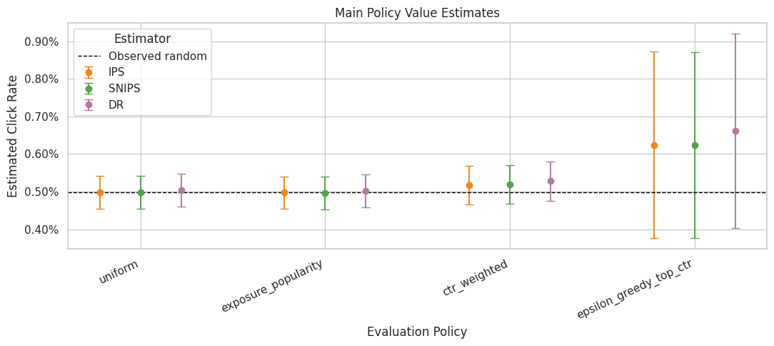

The estimate plot compares policies on the same offline value scale. Error bars and estimator differences are just as important as the ranking, because high-variance estimates should not drive product decisions alone.

Weight Clipping Sensitivity

This section checks whether conclusions depend on extreme importance weights.

We estimate the same policies with no clipping and with weight caps at 5, 10, and 20. Clipping can reduce variance, but it also changes the estimand by shrinking the influence of rare high-weight rows. A robust policy conclusion should not flip wildly across reasonable clipping thresholds.

clip_values = [None, 5, 10, 20]
clipping_frames = []
for clip in clip_values:
    estimates, metrics, _, _ = run_ope_for_split(
        main_train_df,
        main_eval_df,
        model_name="lightgbm",
        split_name="main_50_50",
        clip=clip,
    )
    clipping_frames.append(estimates)

clipping_sensitivity = pd.concat(clipping_frames, ignore_index=True)
clipping_sensitivity["lift_pp"] = 100 * (
    clipping_sensitivity["estimate"] - clipping_sensitivity["eval_observed_click_rate"]
)

clipping_sensitivity.query("estimator in ['IPS', 'SNIPS', 'DR']").head(12)

	split_name	reward_model	policy	estimator	clip	estimate	se	ci_95_lower	ci_95_upper	ess_share	mean_weight	max_weight	p99_weight	mean_abs_correction	mean_correction	eval_observed_click_rate	lift_pp
0	main_50_50	lightgbm	uniform	IPS	none	0.004980	0.000223	0.004544	0.005416	1.000000	1.000000	1.000000	1.000000	0.009856	0.000048	0.004980	0.000000
1	main_50_50	lightgbm	uniform	SNIPS	none	0.004980	0.000223	0.004544	0.005416	1.000000	1.000000	1.000000	1.000000	0.009856	0.000048	0.004980	0.000000
3	main_50_50	lightgbm	uniform	DR	none	0.005034	0.000226	0.004592	0.005476	1.000000	1.000000	1.000000	1.000000	0.009856	0.000048	0.004980	0.005411
4	main_50_50	lightgbm	exposure_popularity	IPS	none	0.004971	0.000223	0.004535	0.005407	0.996399	1.000591	1.132200	1.132200	0.009821	0.000064	0.004980	-0.000904
5	main_50_50	lightgbm	exposure_popularity	SNIPS	none	0.004968	0.000223	0.004532	0.005404	0.996399	1.000591	1.132200	1.132200	0.009821	0.000064	0.004980	-0.001198
7	main_50_50	lightgbm	exposure_popularity	DR	none	0.005020	0.000226	0.004578	0.005462	0.996399	1.000591	1.132200	1.132200	0.009821	0.000064	0.004980	0.003997
8	main_50_50	lightgbm	ctr_weighted	IPS	none	0.005172	0.000261	0.004660	0.005685	0.790628	0.996987	2.740842	2.740842	0.011042	-0.000766	0.004980	0.019244
9	main_50_50	lightgbm	ctr_weighted	SNIPS	none	0.005188	0.000262	0.004675	0.005701	0.790628	0.996987	2.740842	2.740842	0.011042	-0.000766	0.004980	0.020806
11	main_50_50	lightgbm	ctr_weighted	DR	none	0.005282	0.000267	0.004759	0.005805	0.790628	0.996987	2.740842	2.740842	0.011042	-0.000766	0.004980	0.030172
12	main_50_50	lightgbm	epsilon_greedy_top_ctr	IPS	none	0.006238	0.001267	0.003756	0.008720	0.040290	1.001105	29.050000	29.050000	0.017369	-0.005016	0.004980	0.125800
13	main_50_50	lightgbm	epsilon_greedy_top_ctr	SNIPS	none	0.006231	0.001261	0.003759	0.008703	0.040290	1.001105	29.050000	29.050000	0.017369	-0.005016	0.004980	0.125111
15	main_50_50	lightgbm	epsilon_greedy_top_ctr	DR	none	0.006622	0.001320	0.004035	0.009209	0.040290	1.001105	29.050000	29.050000	0.017369	-0.005016	0.004980	0.164171

The clipping sensitivity check shows how estimates change when extreme weights are capped. Stable estimates across clipping thresholds are more reassuring than estimates that depend strongly on a few high-weight rows.

Plot Clipping Sensitivity

This plot shows how the estimated policy value changes as the clipping threshold changes.

The most important line is the DR line, because DR is the preferred estimator after Notebook 4. IPS is included to show why clipping matters more for pure importance weighting. SNIPS is included as a stabilizing benchmark.

clipping_plot = clipping_sensitivity.query("estimator in ['IPS', 'SNIPS', 'DR']").copy()
clipping_plot["clip_label"] = clipping_plot["clip"].astype(str)

fig, ax = plt.subplots(figsize=(11, 5))
sns.lineplot(
    data=clipping_plot,
    x="clip_label",
    y="estimate",
    hue="policy",
    style="estimator",
    marker="o",
    ax=ax,
)
ax.set_title("Policy Value Sensitivity To Weight Clipping")
ax.set_xlabel("Weight Clip")
ax.set_ylabel("Estimated Click Rate")
ax.yaxis.set_major_formatter(lambda y, _: f"{y:.2%}")
plt.tight_layout()
plt.show()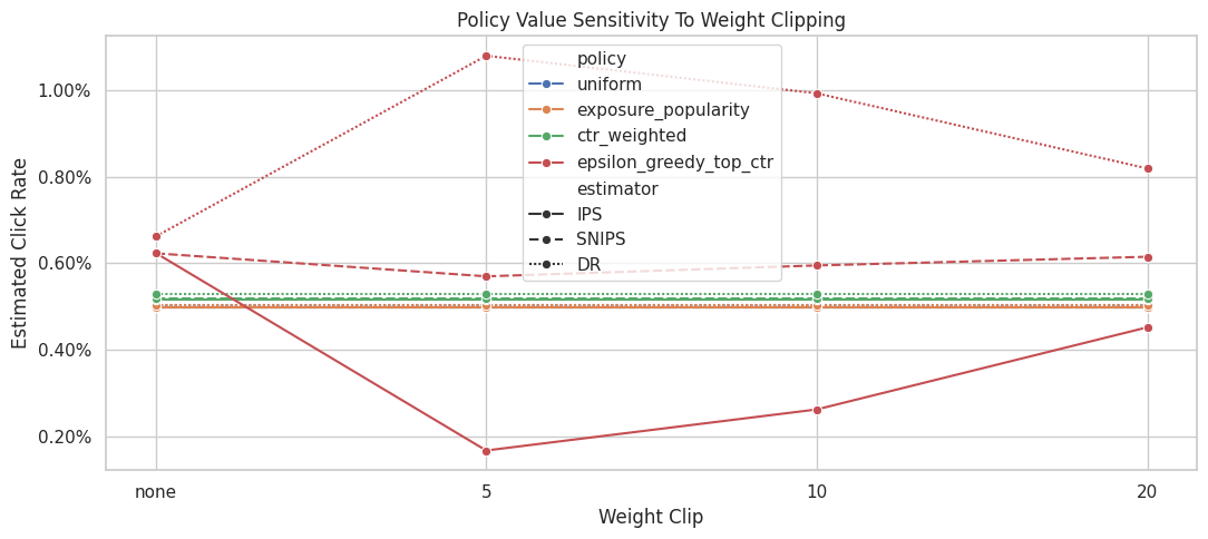

The clipping sensitivity check shows how estimates change when extreme weights are capped. Stable estimates across clipping thresholds are more reassuring than estimates that depend strongly on a few high-weight rows.

Clipping Stability Summary

This cell summarizes how much each policy-estimator estimate moves across clipping thresholds.

estimate_range is the difference between the largest and smallest estimate across the clipping settings. Smaller ranges indicate more stable estimates. Large ranges indicate that extreme weights are influencing the result.

clipping_stability = (
    clipping_sensitivity.query("estimator in ['IPS', 'SNIPS', 'DR']")
    .groupby(["policy", "estimator"])
    .agg(
        min_estimate=("estimate", "min"),
        max_estimate=("estimate", "max"),
        estimate_range=("estimate", lambda x: x.max() - x.min()),
        min_ess_share=("ess_share", "min"),
        max_weight=("max_weight", "max"),
    )
    .reset_index()
    .sort_values("estimate_range", ascending=False)
)

clipping_stability

	policy	estimator	min_estimate	max_estimate	estimate_range	min_ess_share	max_weight
4	epsilon_greedy_top_ctr	IPS	0.001669	0.006238	0.004570	0.040290	29.050000
3	epsilon_greedy_top_ctr	DR	0.006622	0.010802	0.004180	0.040290	29.050000
5	epsilon_greedy_top_ctr	SNIPS	0.005698	0.006231	0.000533	0.040290	29.050000
0	ctr_weighted	DR	0.005282	0.005282	0.000000	0.790628	2.740842
2	ctr_weighted	SNIPS	0.005188	0.005188	0.000000	0.790628	2.740842
1	ctr_weighted	IPS	0.005172	0.005172	0.000000	0.790628	2.740842
6	exposure_popularity	DR	0.005020	0.005020	0.000000	0.996399	1.132200
7	exposure_popularity	IPS	0.004971	0.004971	0.000000	0.996399	1.132200
8	exposure_popularity	SNIPS	0.004968	0.004968	0.000000	0.996399	1.132200
9	uniform	DR	0.005034	0.005034	0.000000	1.000000	1.000000
10	uniform	IPS	0.004980	0.004980	0.000000	1.000000	1.000000
11	uniform	SNIPS	0.004980	0.004980	0.000000	1.000000	1.000000

The clipping sensitivity check shows how estimates change when extreme weights are capped. Stable estimates across clipping thresholds are more reassuring than estimates that depend strongly on a few high-weight rows.

Reward Model Sensitivity

This section checks whether doubly robust estimates depend heavily on the reward model.

We compare three reward-model specifications:

• logistic regression
• a shallow LightGBM model
• the main LightGBM model

If DR estimates are broadly consistent across these models, that supports the policy conclusion. If rankings change sharply, the final recommendation should be framed as more tentative.

reward_model_names = ["logistic", "lightgbm_shallow", "lightgbm"]
reward_model_estimate_frames = []
reward_model_metric_frames = []

for model_name in reward_model_names:
    estimates, metrics, _, _ = run_ope_for_split(
        main_train_df,
        main_eval_df,
        model_name=model_name,
        split_name="main_50_50",
        clip=None,
    )
    reward_model_estimate_frames.append(estimates)
    reward_model_metric_frames.append(metrics)

reward_model_sensitivity = pd.concat(reward_model_estimate_frames, ignore_index=True)
reward_model_metrics = pd.concat(reward_model_metric_frames, ignore_index=True)

reward_model_metrics.sort_values("log_loss")

	split_name	reward_model	train_rows	eval_rows	auc	average_precision	log_loss	brier_score	mean_prediction	observed_click_rate
0	main_50_50	logistic	100000	100000	0.539928	0.006395	0.032528	0.005081	0.005774	0.004980
1	main_50_50	lightgbm_shallow	100000	100000	0.541724	0.006571	0.032535	0.005020	0.005315	0.004980
2	main_50_50	lightgbm	100000	100000	0.534265	0.005821	0.034100	0.005096	0.004932	0.004980

Reward-model sensitivity checks whether DR conclusions depend on a particular predictive model. Stable rankings across model classes make the recommendation more credible.

Plot Reward Model Sensitivity For DR

This plot compares DR estimates across reward models.

The DR estimator still uses the same logged propensities and the same evaluation policies. The only changing ingredient is the reward model used for the direct component and residual prediction. Stable DR estimates across models are a good sign.

dr_model_plot = reward_model_sensitivity.query("estimator == 'DR'").copy()

fig, ax = plt.subplots(figsize=(10, 5))
sns.pointplot(
    data=dr_model_plot,
    x="policy",
    y="estimate",
    hue="reward_model",
    dodge=0.35,
    errorbar=None,
    ax=ax,
)
ax.axhline(main_eval_df["click"].mean(), color="black", linestyle="--", linewidth=1, label="Observed random")
ax.set_title("DR Estimate Sensitivity To Reward Model")
ax.set_xlabel("Evaluation Policy")
ax.set_ylabel("Estimated Click Rate")
ax.tick_params(axis="x", rotation=25)
ax.yaxis.set_major_formatter(lambda y, _: f"{y:.2%}")
plt.tight_layout()
plt.show()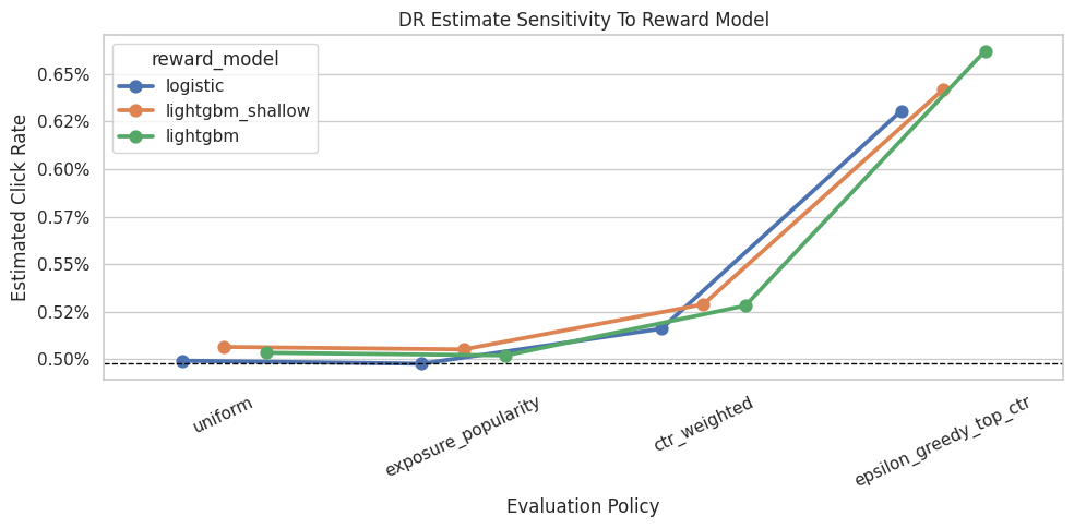

Reward-model sensitivity checks whether DR conclusions depend on a particular predictive model. Stable rankings across model classes make the recommendation more credible.

Reward Model Ranking Stability

This cell converts reward-model sensitivity into policy ranks.

Rank 1 is the highest DR estimate within a reward model. If the same policy remains near the top across reward models, the recommendation is more robust. If the top policy changes completely, we should be cautious.

reward_model_rank_stability = dr_model_plot.copy()
reward_model_rank_stability["rank_within_model"] = reward_model_rank_stability.groupby("reward_model")["estimate"].rank(
    ascending=False, method="min"
)

reward_model_rank_summary = (
    reward_model_rank_stability.groupby("policy")
    .agg(
        avg_rank_across_models=("rank_within_model", "mean"),
        best_rank_across_models=("rank_within_model", "min"),
        worst_rank_across_models=("rank_within_model", "max"),
        estimate_range_across_models=("estimate", lambda x: x.max() - x.min()),
    )
    .reset_index()
    .sort_values(["avg_rank_across_models", "estimate_range_across_models"])
)

reward_model_rank_summary

	policy	avg_rank_across_models	best_rank_across_models	worst_rank_across_models	estimate_range_across_models
1	epsilon_greedy_top_ctr	1.000000	1.000000	1.000000	0.000315
0	ctr_weighted	2.000000	2.000000	2.000000	0.000128
3	uniform	3.000000	3.000000	3.000000	0.000073
2	exposure_popularity	4.000000	4.000000	4.000000	0.000075

The stability summary focuses on whether policy rankings change under reasonable analysis choices. A policy that remains near the top across checks is a stronger offline candidate than one that wins only under one specification.

Time Split Sensitivity

This section repeats the DR analysis across different time windows.

Each split uses an earlier block of data for training and a later block for evaluation. This tests whether the best policy is stable across time or whether it only looks good in one particular held-out window.

To keep runtime reasonable, the evaluation windows are shorter than the main 50/50 evaluation split.

split_specs = [
    {"split_name": "early_window", "train_start": 0.00, "train_end": 0.40, "eval_start": 0.40, "eval_end": 0.55},
    {"split_name": "middle_window", "train_start": 0.00, "train_end": 0.50, "eval_start": 0.50, "eval_end": 0.65},
    {"split_name": "late_window", "train_start": 0.00, "train_end": 0.60, "eval_start": 0.60, "eval_end": 0.75},
]

split_plan = []
for spec in split_specs:
    n = len(random_df)
    train_start = int(n * spec["train_start"])
    train_end = int(n * spec["train_end"])
    eval_start = int(n * spec["eval_start"])
    eval_end = int(n * spec["eval_end"])
    split_plan.append(
        {
            "split_name": spec["split_name"],
            "train_rows": train_end - train_start,
            "eval_rows": eval_end - eval_start,
            "train_start_time": random_df.iloc[train_start]["timestamp"],
            "train_end_time": random_df.iloc[train_end - 1]["timestamp"],
            "eval_start_time": random_df.iloc[eval_start]["timestamp"],
            "eval_end_time": random_df.iloc[eval_end - 1]["timestamp"],
        }
    )

pd.DataFrame(split_plan)

	split_name	train_rows	eval_rows	train_start_time	train_end_time	eval_start_time	eval_end_time
0	early_window	80000	30000	2019-11-24 00:00:03.800821+00:00	2019-11-25 01:13:20.340362+00:00	2019-11-25 01:13:23.467887+00:00	2019-11-25 12:31:38.942417+00:00
1	middle_window	100000	30000	2019-11-24 00:00:03.800821+00:00	2019-11-25 10:01:18.392921+00:00	2019-11-25 10:01:18.393450+00:00	2019-11-25 19:24:35.095071+00:00
2	late_window	120000	30000	2019-11-24 00:00:03.800821+00:00	2019-11-25 14:22:22.600427+00:00	2019-11-25 14:22:22.600570+00:00	2019-11-26 06:51:42.575935+00:00

Time-split sensitivity checks whether the offline conclusion changes across different train/evaluation windows. This is important because recommendation environments can drift over time.

Run Split Sensitivity Estimates

This cell runs LightGBM DR estimates for each time split.

The split loop rebuilds policies and retrains the reward model inside each time window. That is intentional: it tests the full workflow, not just the final estimator on a fixed policy.

split_estimate_frames = []
split_metric_frames = []

for spec in split_specs:
    n = len(random_df)
    train_df = random_df.iloc[int(n * spec["train_start"]) : int(n * spec["train_end"])].copy()
    eval_df = random_df.iloc[int(n * spec["eval_start"]) : int(n * spec["eval_end"])].copy()

    estimates, metrics, _, _ = run_ope_for_split(
        train_df,
        eval_df,
        model_name="lightgbm",
        split_name=spec["split_name"],
        clip=None,
    )
    split_estimate_frames.append(estimates)
    split_metric_frames.append(metrics)

split_sensitivity = pd.concat(split_estimate_frames, ignore_index=True)
split_model_metrics = pd.concat(split_metric_frames, ignore_index=True)

split_model_metrics

	split_name	reward_model	train_rows	eval_rows	auc	average_precision	log_loss	brier_score	mean_prediction	observed_click_rate
0	early_window	lightgbm	80000	30000	0.540994	0.004299	0.027959	0.004138	0.004624	0.003967
1	middle_window	lightgbm	100000	30000	0.572556	0.009731	0.034497	0.005294	0.005305	0.005167
2	late_window	lightgbm	120000	30000	0.507023	0.006752	0.036425	0.005458	0.004942	0.005367

Time-split sensitivity checks whether the offline conclusion changes across different train/evaluation windows. This is important because recommendation environments can drift over time.

Plot Split Sensitivity For DR

This plot shows DR estimates across time windows.

A stable policy should remain competitive across early, middle, and late windows. A policy that only wins in one split may still be interesting, but it is a weaker candidate for a confident offline recommendation.

split_dr_plot = split_sensitivity.query("estimator == 'DR'").copy()

fig, ax = plt.subplots(figsize=(10, 5))
sns.lineplot(
    data=split_dr_plot,
    x="split_name",
    y="estimate",
    hue="policy",
    marker="o",
    ax=ax,
)
ax.set_title("DR Estimate Stability Across Time Splits")
ax.set_xlabel("Time Split")
ax.set_ylabel("Estimated Click Rate")
ax.yaxis.set_major_formatter(lambda y, _: f"{y:.2%}")
plt.tight_layout()
plt.show()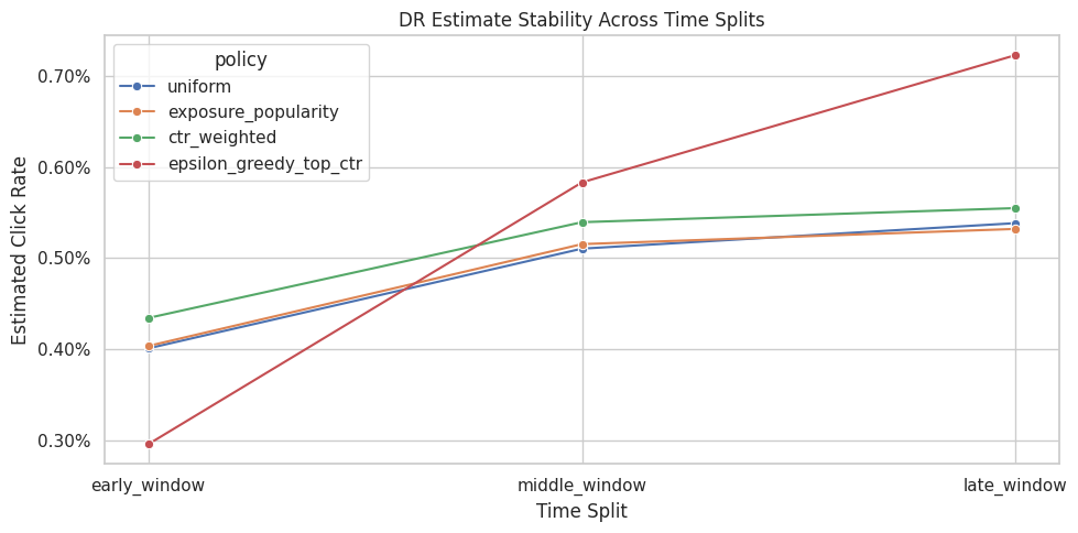

Time-split sensitivity checks whether the offline conclusion changes across different train/evaluation windows. This is important because recommendation environments can drift over time.

Split Ranking Stability

This cell ranks policies within each time split using the LightGBM DR estimate.

The rank summary is more robust than staring only at point estimates. A policy with average rank near 1 and low rank standard deviation is a stable offline winner.

split_rank_table = split_dr_plot.copy()
split_rank_table["rank_within_split"] = split_rank_table.groupby("split_name")["estimate"].rank(
    ascending=False, method="min"
)

split_rank_summary = (
    split_rank_table.groupby("policy")
    .agg(
        avg_rank_across_splits=("rank_within_split", "mean"),
        rank_std_across_splits=("rank_within_split", "std"),
        best_rank_across_splits=("rank_within_split", "min"),
        worst_rank_across_splits=("rank_within_split", "max"),
        mean_dr_estimate_across_splits=("estimate", "mean"),
        dr_estimate_range_across_splits=("estimate", lambda x: x.max() - x.min()),
    )
    .reset_index()
    .sort_values(["avg_rank_across_splits", "dr_estimate_range_across_splits"])
)

split_rank_summary

	policy	avg_rank_across_splits	rank_std_across_splits	best_rank_across_splits	worst_rank_across_splits	mean_dr_estimate_across_splits	dr_estimate_range_across_splits
0	ctr_weighted	1.666667	0.577350	1.000000	2.000000	0.005094	0.001205
1	epsilon_greedy_top_ctr	2.000000	1.732051	1.000000	4.000000	0.005338	0.004269
2	exposure_popularity	3.000000	1.000000	2.000000	4.000000	0.004836	0.001285
3	uniform	3.333333	0.577350	3.000000	4.000000	0.004831	0.001374

The split separates policy construction from policy evaluation. This prevents using the same rows to design a policy and evaluate it, which would make the offline result too optimistic.

Build A Policy Risk Table

This cell combines the main LightGBM DR estimate with support, clipping stability, reward-model stability, and split stability.

This is the most decision-oriented table in the notebook. It tries to answer: which policy has strong estimated value and enough stability to justify an online experiment?

main_dr = main_lgbm_table.query("estimator == 'DR'").copy()
main_dr = main_dr[
    [
        "policy",
        "estimate",
        "ci_95_lower",
        "ci_95_upper",
        "lift_pp",
        "relative_lift_pct",
        "ess_share",
        "mean_weight",
        "max_weight",
        "p99_weight",
        "mean_abs_correction",
    ]
]

clip_dr_stability = clipping_stability.query("estimator == 'DR'")[["policy", "estimate_range"]].rename(
    columns={"estimate_range": "dr_clip_estimate_range"}
)

policy_risk_table = (
    main_dr.merge(clip_dr_stability, on="policy", how="left")
    .merge(reward_model_rank_summary, on="policy", how="left")
    .merge(split_rank_summary, on="policy", how="left")
)

policy_risk_table["decision_score"] = (
    policy_risk_table["lift_pp"]
    - 0.25 * policy_risk_table["avg_rank_across_splits"]
    - 100 * policy_risk_table["dr_clip_estimate_range"]
    - 0.10 * policy_risk_table["max_weight"]
)

policy_risk_table.sort_values("decision_score", ascending=False)

	policy	estimate	ci_95_lower	ci_95_upper	lift_pp	relative_lift_pct	ess_share	mean_weight	max_weight	p99_weight	mean_abs_correction	dr_clip_estimate_range	avg_rank_across_models	best_rank_across_models	worst_rank_across_models	estimate_range_across_models	avg_rank_across_splits	rank_std_across_splits	best_rank_across_splits	worst_rank_across_splits	mean_dr_estimate_across_splits	dr_estimate_range_across_splits	decision_score
2	ctr_weighted	0.005282	0.004759	0.005805	0.030172	6.058681	0.790628	0.996987	2.740842	2.740842	0.011042	0.000000	2.000000	2.000000	2.000000	0.000128	1.666667	0.577350	1.000000	2.000000	0.005094	0.001205	-0.660579
1	exposure_popularity	0.005020	0.004578	0.005462	0.003997	0.802658	0.996399	1.000591	1.132200	1.132200	0.009821	0.000000	4.000000	4.000000	4.000000	0.000075	3.000000	1.000000	2.000000	4.000000	0.004836	0.001285	-0.859223
0	uniform	0.005034	0.004592	0.005476	0.005411	1.086540	1.000000	1.000000	1.000000	1.000000	0.009856	0.000000	3.000000	3.000000	3.000000	0.000073	3.333333	0.577350	3.000000	4.000000	0.004831	0.001374	-0.927922
3	epsilon_greedy_top_ctr	0.006622	0.004035	0.009209	0.164171	32.966042	0.040290	1.001105	29.050000	29.050000	0.017369	0.004180	1.000000	1.000000	1.000000	0.000315	2.000000	1.732051	1.000000	4.000000	0.005338	0.004269	-3.658854

The policy-risk table combines value, lift, support, and stability into a decision-oriented view. This is closer to how an experimentation team would decide what is safe enough to test online.

Choose An Offline Candidate For A/B Testing

This cell selects a candidate policy using the policy risk table.

The selection is intentionally conservative. It does not simply choose the highest point estimate. It sorts by a decision score that rewards estimated lift and penalizes poor split rank, clipping instability, and large maximum weights.

This is not an automated production rule. It is a transparent way to make the offline recommendation auditable.

recommended_policy_row = policy_risk_table.sort_values("decision_score", ascending=False).iloc[0]
recommended_policy = recommended_policy_row["policy"]

recommendation_summary = pd.Series(
    {
        "recommended_policy_for_ab_test": recommended_policy,
        "dr_estimated_click_rate": recommended_policy_row["estimate"],
        "lift_pp_vs_random_behavior": recommended_policy_row["lift_pp"],
        "relative_lift_pct_vs_random_behavior": recommended_policy_row["relative_lift_pct"],
        "ess_share": recommended_policy_row["ess_share"],
        "max_weight": recommended_policy_row["max_weight"],
        "avg_rank_across_splits": recommended_policy_row["avg_rank_across_splits"],
        "avg_rank_across_reward_models": recommended_policy_row["avg_rank_across_models"],
        "decision_score": recommended_policy_row["decision_score"],
    }
).to_frame("value")

recommendation_summary

	value
recommended_policy_for_ab_test	ctr_weighted
dr_estimated_click_rate	0.005282
lift_pp_vs_random_behavior	0.030172
relative_lift_pct_vs_random_behavior	6.058681
ess_share	0.790628
max_weight	2.740842
avg_rank_across_splits	1.666667
avg_rank_across_reward_models	2.000000
decision_score	-0.660579

The recommended candidate is selected from the offline evidence, not from value alone. The decision should balance estimated improvement against support risk, uncertainty, and robustness.

What We Would And Would Not Claim

This cell writes the final interpretation in plain English.

A strong portfolio project should be explicit about limitations. Offline OPE can recommend which policy is worth testing, but it should not be framed as proof that the policy will win in production. Online experimentation is still needed.

interpretation_text = f"""
Recommended offline candidate: {recommended_policy}

Why this policy is credible:
- It has a competitive LightGBM doubly robust estimate on the main held-out split.
- Its effective sample size and maximum weight are part of the decision table, so the recommendation is not based on point estimate alone.
- It was compared across clipping thresholds, reward-model choices, and time windows.

What this does not prove:
- It does not prove the policy would win in production.
- It does not account for long-term user effects, novelty fatigue, marketplace effects, or interference across items.
- It assumes the Open Bandit logged propensities are correct and that the random log has support for the evaluation policies.

Operational recommendation:
Use this policy as the strongest offline candidate for an online A/B test, with guardrail metrics for click quality, downstream engagement, and user experience.
""".strip()

print(interpretation_text)

Recommended offline candidate: ctr_weighted

Why this policy is credible:
- It has a competitive LightGBM doubly robust estimate on the main held-out split.
- Its effective sample size and maximum weight are part of the decision table, so the recommendation is not based on point estimate alone.
- It was compared across clipping thresholds, reward-model choices, and time windows.

What this does not prove:
- It does not prove the policy would win in production.
- It does not account for long-term user effects, novelty fatigue, marketplace effects, or interference across items.
- It assumes the Open Bandit logged propensities are correct and that the random log has support for the evaluation policies.

Operational recommendation:
Use this policy as the strongest offline candidate for an online A/B test, with guardrail metrics for click quality, downstream engagement, and user experience.

This text cell is the guardrail against overclaiming. Offline evaluation can recommend candidates for online testing, but it cannot replace an A/B test when business-critical deployment decisions are at stake.

Save Sensitivity Tables

This final code cell saves the most important sensitivity outputs to a small writeup folder inside the off-policy evaluation notebook directory.

These tables make it easier to build a final report later without rerunning the full notebook every time.

WRITEUP_DIR = PROJECT_ROOT / "notebooks/projects/project_2_off_policy_evaluation/writeup"
TABLE_DIR = WRITEUP_DIR / "tables"
TABLE_DIR.mkdir(parents=True, exist_ok=True)

main_lgbm_table.to_csv(TABLE_DIR / "main_lgbm_ope_estimates.csv", index=False)
clipping_stability.to_csv(TABLE_DIR / "clipping_stability.csv", index=False)
reward_model_rank_summary.to_csv(TABLE_DIR / "reward_model_rank_stability.csv", index=False)
split_rank_summary.to_csv(TABLE_DIR / "split_rank_stability.csv", index=False)
policy_risk_table.to_csv(TABLE_DIR / "policy_risk_table.csv", index=False)

artifact_table = pd.DataFrame(
    {
        "path": [str(path.relative_to(PROJECT_ROOT)) for path in sorted(TABLE_DIR.glob("*.csv"))],
        "size_kb": [path.stat().st_size / 1024 for path in sorted(TABLE_DIR.glob("*.csv"))],
    }
)

artifact_table

	path	size_kb
0	notebooks/projects/project_2_off_policy_evaluation/writeup/tables...	1.283203
1	notebooks/projects/project_2_off_policy_evaluation/writeup/tables...	4.750000
2	notebooks/projects/project_2_off_policy_evaluation/writeup/tables...	1.785156
3	notebooks/projects/project_2_off_policy_evaluation/writeup/tables...	0.300781
4	notebooks/projects/project_2_off_policy_evaluation/writeup/tables...	0.527344

This cell saves reusable outputs for downstream notebooks or the final writeup. Persisting these artifacts makes the project modular and prevents later notebooks from repeating expensive or fragile setup work.

Notebook 5 Takeaways

This notebook stress-tested the policy recommendation rather than trusting one estimator run.

The decision process now includes:

• main LightGBM DR estimates
• IPS and SNIPS benchmarks
• clipping sensitivity
• reward-model sensitivity
• time-split sensitivity
• policy support diagnostics
• a policy risk table

The final offline output should be framed as: which policy is most justified for an online A/B test, not which policy is guaranteed to be best in production.

A good next step would be a short final report notebook that turns the off-policy evaluation results into clean figures, tables, and interview-ready writing.