from pathlib import Path
import warnings

import lightgbm as lgb
import matplotlib.pyplot as plt
import numpy as np
import pandas as pd
import seaborn as sns
from sklearn.compose import ColumnTransformer
from sklearn.linear_model import LogisticRegression
from sklearn.metrics import average_precision_score, brier_score_loss, log_loss, roc_auc_score
from sklearn.pipeline import Pipeline
from sklearn.preprocessing import OneHotEncoder, StandardScaler

pd.set_option("display.max_columns", 120)
pd.set_option("display.max_rows", 120)
pd.set_option("display.float_format", "{:.6f}".format)

sns.set_theme(style="whitegrid", context="notebook")

warnings.filterwarnings(
    "ignore",
    message="X does not have valid feature names, but LGBMClassifier was fitted with feature names",
    category=UserWarning,
)04 Doubly Robust Off-Policy Evaluation
This notebook upgrades the analysis from pure importance weighting to doubly robust off-policy evaluation.
Notebook 3 estimated policy values with IPS and SNIPS. Those estimators are valuable because they use the known logging propensities directly, but they can become noisy when importance weights are large or concentrated. Doubly robust OPE adds a second ingredient: a reward model.
The reward model estimates:
q(x, a) = E[Y | X = x, A = a]
For this project, Y is click, X is recommendation context, and A is the recommended item. The doubly robust estimator combines:
- a model-based prediction of what each policy would get in each context
- an IPS-style correction for the residual error on the action that was actually logged
This notebook keeps the same evaluation policies from Notebook 3 so that the comparison is clear: IPS, SNIPS, direct method, and doubly robust estimates are all answering the same policy-value question.
Why Doubly Robust OPE?
IPS estimates policy value by weighting observed rewards:
mean((pi_e(A|X) / pi_b(A|X)) * Y)
This is powerful because it does not require a reward model, but it can be high variance. If the behavior policy rarely chose an action that the evaluation policy likes, the importance weight can become large.
The direct method takes the opposite approach. It trains a reward model q_hat(x, a) and estimates policy value by averaging predicted rewards under the evaluation policy:
mean(sum_a pi_e(a|x) * q_hat(x, a))
The direct method can be stable, but it is biased if the reward model is wrong.
The doubly robust estimator combines both:
mean(sum_a pi_e(a|x) * q_hat(x, a) + (pi_e(A|X) / pi_b(A|X)) * (Y - q_hat(X, A)))
The first term is the model-based policy value. The second term corrects the model using observed residuals on logged actions. It is called doubly robust because, under standard assumptions, it can remain consistent if either the propensities are correct or the reward model is correct.
Notebook Setup
This cell imports data, modeling, evaluation, and plotting libraries. It also suppresses one known LightGBM/sklearn feature-name metadata warning so the notebook output stays readable while real warnings remain visible.
We train two reward models:
- logistic regression as a transparent baseline
- LightGBM as a stronger nonlinear model
Using both models is useful because doubly robust OPE should not be treated as a black box. If DR estimates move sharply across reward models, that is a sensitivity warning.
This cell prepares the notebook environment for doubly robust off-policy evaluation. There is no estimator output yet; the main value is that the imports, display settings, and plotting defaults are ready for the OPE diagnostics that follow.
Locate The Cached Open Bandit Sample
This cell finds the repository root and loads the random-policy sample created in Notebook 1.
We use the random-policy log for the main DR estimates because Notebook 2 showed that it has broad support and stable propensities. This makes it the cleanest source for introducing a reward model and doubly robust correction.
RANDOM_SAMPLE_RELATIVE_PATH = Path("data/processed/open_bandit_random_men_sample.parquet")
PROJECT_ROOT = next(
    path
    for path in [Path.cwd(), *Path.cwd().parents]
    if (path / RANDOM_SAMPLE_RELATIVE_PATH).exists()
)

RANDOM_SAMPLE_PATH = PROJECT_ROOT / RANDOM_SAMPLE_RELATIVE_PATH
random_df = pd.read_parquet(RANDOM_SAMPLE_PATH).sort_values("timestamp").reset_index(drop=True)

pd.Series(
    {
        "project_root": PROJECT_ROOT,
        "random_sample_path": RANDOM_SAMPLE_PATH,
        "rows": len(random_df),
        "columns": random_df.shape[1],
        "observed_click_rate": random_df["click"].mean(),
    }
).to_frame("value")| value | |
|---|---|
| project_root | /home/apex/Documents/ranking_sys |
| random_sample_path | /home/apex/Documents/ranking_sys/data/processe... |
| rows | 200000 |
| columns | 50 |
| observed_click_rate | 0.005190 |
The printed paths are a reproducibility checkpoint. Once the notebook can find the cached data and writeup folders, the rest of the analysis can run without manual path edits.
Recreate The Train And Evaluation Split
To stay aligned with Notebook 3, this notebook uses the same time-based split:
- the first half of rows defines policies and trains reward models
- the second half evaluates policy values
This separation matters. We should not tune a policy or reward model on the exact same rows used for final OPE without acknowledging the risk of overfitting.
SPLIT_FRACTION = 0.50
split_idx = int(len(random_df) * SPLIT_FRACTION)

train_df = random_df.iloc[:split_idx].copy()
eval_df = random_df.iloc[split_idx:].copy()

split_summary = pd.DataFrame(
    {
        "split": ["train", "evaluation"],
        "rows": [len(train_df), len(eval_df)],
        "min_timestamp": [train_df["timestamp"].min(), eval_df["timestamp"].min()],
        "max_timestamp": [train_df["timestamp"].max(), eval_df["timestamp"].max()],
        "click_rate": [train_df["click"].mean(), eval_df["click"].mean()],
    }
)

split_summary| split | rows | min_timestamp | max_timestamp | click_rate | |
|---|---|---|---|---|---|
| 0 | train | 100000 | 2019-11-24 00:00:03.800821+00:00 | 2019-11-25 10:01:18.392921+00:00 | 0.005400 |
| 1 | evaluation | 100000 | 2019-11-25 10:01:18.393450+00:00 | 2019-11-27 02:50:16.027289+00:00 | 0.004980 |
The split separates policy construction from policy evaluation. This prevents using the same rows to design a policy and evaluate it, which would make the offline result too optimistic.
Define The Action Space And Feature Groups
The action is the recommended item. In the men campaign there are 34 item actions.
For reward modeling, we build features that are available before the click outcome:
- user categorical features
- recommendation position and hour
- candidate item ID
- candidate item metadata
- selected user-item affinity for the candidate item
The selected affinity is important. The raw log has one affinity column per item. When we score a candidate action, we use the affinity column corresponding to that candidate item.
action_space = np.array(sorted(random_df["item_id"].unique()))
n_actions = len(action_space)

user_feature_cols = [col for col in random_df.columns if col.startswith("user_feature_")]
affinity_cols_by_action = [f"user-item_affinity_{item_id}" for item_id in action_space]
item_feature_cols = [col for col in random_df.columns if col.startswith("item_feature_")]

categorical_features = [
    "position",
    "hour",
    "item_id",
    *user_feature_cols,
    "item_feature_1",
    "item_feature_2",
    "item_feature_3",
]
numeric_features = ["selected_affinity", "item_feature_0"]
feature_cols = categorical_features + numeric_features

feature_group_summary = pd.DataFrame(
    {
        "group": ["actions", "user categorical", "item metadata", "model categorical", "model numeric"],
        "count": [n_actions, len(user_feature_cols), len(item_feature_cols), len(categorical_features), len(numeric_features)],
        "columns": [list(action_space), user_feature_cols, item_feature_cols, categorical_features, numeric_features],
    }
)

feature_group_summary| group | count | columns | |
|---|---|---|---|
| 0 | actions | 34 | [0, 1, 2, 3, 4, 5, 6, 7, 8, 9, 10, 11, 12, 13,... |
| 1 | user categorical | 4 | [user_feature_0, user_feature_1, user_feature_... |
| 2 | item metadata | 4 | [item_feature_0, item_feature_1, item_feature_... |
| 3 | model categorical | 10 | [position, hour, item_id, user_feature_0, user... |
| 4 | model numeric | 2 | [selected_affinity, item_feature_0] |
The action-space definition fixes the set of items that evaluation policies are allowed to choose. OPE estimates are only meaningful for policies whose action probabilities live inside this logged support.
Build Item Metadata Lookup
The cached random sample already contains item metadata for the logged item. To score counterfactual candidate actions, we need one metadata row per item.
This cell builds an item lookup table. Later, when we score item a for a context, we attach the metadata for item a, not the metadata for the item that happened to be logged in that row.
item_context = (
    random_df[["item_id", *item_feature_cols]]
    .drop_duplicates("item_id")
    .set_index("item_id")
    .sort_index()
)

missing_items = sorted(set(action_space) - set(item_context.index))
if missing_items:
    raise ValueError(f"Missing item metadata for item IDs: {missing_items}")

item_context.head()| item_feature_0 | item_feature_1 | item_feature_2 | item_feature_3 | |
|---|---|---|---|---|
| item_id | ||||
| 0 | -0.677183 | ce58bf66d7e62186e6ce01bafeea9d39 | 7c5498711d69681385d21c0e26923e7e | bbf748c6c978938bc63d432efa60191c |
| 1 | -0.720300 | 3c2985d744e0d57c261abd7e541e4263 | 7c5498711d69681385d21c0e26923e7e | bbf748c6c978938bc63d432efa60191c |
| 2 | 0.745662 | 3c2985d744e0d57c261abd7e541e4263 | 2b851c0a9c4a961da8760d5dc747c5a3 | b61cfaadd526b816e3aeb9b7be4b4759 |
| 3 | -0.698741 | 9874ffb54e9b0a269e29bbb2f5328735 | ce1abd8b5d914ba8fe719b453bc5ba3b | 5bc9c86cd1f08a9991670ea97b34f86d |
| 4 | 1.651109 | 01fe2f187e459e6ada960671d2942dfe | b4b5879029fb5f64eeec63cf4f73ef0e | b61cfaadd526b816e3aeb9b7be4b4759 |
These feature-building cells define the context used by reward models. Reward models need both user context and candidate item context so they can predict counterfactual rewards for actions that were not logged.
Create Logged-Action Reward Model Features
This helper creates a supervised-learning frame for rows where the logged action is known.
For each row, selected_affinity is taken from the affinity column that corresponds to the logged item_id. This makes the training data match the counterfactual scoring data we will create later: every feature row represents a specific context-action pair.
def make_logged_feature_frame(df):
    """Create reward-model features for the action that was actually logged."""
    frame = df.copy()
    affinity_matrix = frame[affinity_cols_by_action].to_numpy()
    item_positions = frame["item_id"].map({item_id: idx for idx, item_id in enumerate(action_space)}).to_numpy()
    frame["selected_affinity"] = affinity_matrix[np.arange(len(frame)), item_positions]
    return frame[feature_cols]

X_train = make_logged_feature_frame(train_df)
y_train = train_df["click"].astype(int)
X_eval_logged = make_logged_feature_frame(eval_df)
y_eval = eval_df["click"].astype(int)

X_train.head()| position | hour | item_id | user_feature_0 | user_feature_1 | user_feature_2 | user_feature_3 | item_feature_1 | item_feature_2 | item_feature_3 | selected_affinity | item_feature_0 | |
|---|---|---|---|---|---|---|---|---|---|---|---|---|
| 0 | 1 | 0 | 0 | cef3390ed299c09874189c387777674a | 03a5648a76832f83c859d46bc06cb64a | 2723d2eb8bba04e0362098011fa3997b | c39b0c7dd5d4eb9a18e7db6ba2f258f8 | ce58bf66d7e62186e6ce01bafeea9d39 | 7c5498711d69681385d21c0e26923e7e | bbf748c6c978938bc63d432efa60191c | 0.000000 | -0.677183 |
| 1 | 3 | 0 | 25 | cef3390ed299c09874189c387777674a | 03a5648a76832f83c859d46bc06cb64a | 2723d2eb8bba04e0362098011fa3997b | c39b0c7dd5d4eb9a18e7db6ba2f258f8 | 9874ffb54e9b0a269e29bbb2f5328735 | 7c5498711d69681385d21c0e26923e7e | bbf748c6c978938bc63d432efa60191c | 0.000000 | -0.461600 |
| 2 | 2 | 0 | 23 | cef3390ed299c09874189c387777674a | 03a5648a76832f83c859d46bc06cb64a | 2723d2eb8bba04e0362098011fa3997b | c39b0c7dd5d4eb9a18e7db6ba2f258f8 | 55fe518d85813954c7d9b8a875ff2453 | cc75031396a5aa830885915aa93f49d0 | b61cfaadd526b816e3aeb9b7be4b4759 | 0.000000 | -0.569392 |
| 3 | 1 | 0 | 25 | 1a2b2ad3a7f218a0d709dd9c656fda27 | e3528f5280f04c0031d337da1def86ea | 398773dacf8501ee8f76e3706ccafbba | 47e7dd7d9ccbe31d57ce716dba831d44 | 9874ffb54e9b0a269e29bbb2f5328735 | 7c5498711d69681385d21c0e26923e7e | bbf748c6c978938bc63d432efa60191c | 0.000000 | -0.461600 |
| 4 | 2 | 0 | 30 | 1a2b2ad3a7f218a0d709dd9c656fda27 | e3528f5280f04c0031d337da1def86ea | 398773dacf8501ee8f76e3706ccafbba | 47e7dd7d9ccbe31d57ce716dba831d44 | 61c5d8c2524684aa047e15e172c7e92f | 3f1feafd79578bedf199c459fecc378b | bbf748c6c978938bc63d432efa60191c | 0.000000 | -0.914324 |
This output is part of the doubly robust off-policy evaluation workflow. Read it as a checkpoint that either verifies the log, defines reusable estimator machinery, or produces a diagnostic that motivates the next OPE step.
Check Reward Model Feature Quality
This cell checks missingness and target balance for the reward-model training frame.
Reward modeling is now part of the causal estimator. If feature construction is broken, the direct method and doubly robust estimates will be misleading. This quick check catches obvious issues before model fitting.
feature_quality = pd.DataFrame(
    {
        "feature": feature_cols,
        "missing_rate_train": [X_train[col].isna().mean() for col in feature_cols],
        "missing_rate_eval": [X_eval_logged[col].isna().mean() for col in feature_cols],
        "train_unique_values": [X_train[col].nunique(dropna=False) for col in feature_cols],
    }
)

target_summary = pd.Series(
    {
        "train_rows": len(y_train),
        "eval_rows": len(y_eval),
        "train_click_rate": y_train.mean(),
        "eval_click_rate": y_eval.mean(),
    }
).to_frame("value")

feature_quality, target_summary
( feature missing_rate_train missing_rate_eval \
0 position 0.000000 0.000000
1 hour 0.000000 0.000000
2 item_id 0.000000 0.000000
3 user_feature_0 0.000000 0.000000
4 user_feature_1 0.000000 0.000000
5 user_feature_2 0.000000 0.000000
6 user_feature_3 0.000000 0.000000
7 item_feature_1 0.000000 0.000000
8 item_feature_2 0.000000 0.000000
9 item_feature_3 0.000000 0.000000
10 selected_affinity 0.000000 0.000000
11 item_feature_0 0.000000 0.000000
train_unique_values
0 3
1 24
2 34
3 4
4 6
5 10
6 10
7 7
8 16
9 4
10 4
11 25 ,
value
train_rows 100000.000000
eval_rows 100000.000000
train_click_rate 0.005400
eval_click_rate 0.004980)The feature-quality table checks whether the reward-model inputs are present and informative. If important context fields were missing or constant, direct method and DR estimates would lean on weak predictions.
Define The Preprocessor
This cell defines the preprocessing shared by the reward models.
Categorical features are one-hot encoded. Numeric features are scaled. The final transformed matrix is then passed to logistic regression or LightGBM.
The preprocessing is intentionally standard and auditable. For OPE, a slightly weaker but understandable reward model is often better for a portfolio notebook than a highly tuned model whose behavior is hard to explain.
preprocessor = ColumnTransformer(
    transformers=[
        ("categorical", OneHotEncoder(handle_unknown="ignore"), categorical_features),
        ("numeric", StandardScaler(), numeric_features),
    ],
    remainder="drop",
)
The weight diagnostics show whether each policy value estimate is supported by enough logged data. Policies with large weights or low ESS may look attractive but carry higher offline evaluation risk.
Train Reward Models
This cell trains two reward models.
The logistic regression model is a baseline with a simple functional form. The LightGBM model can capture nonlinear interactions between context, item metadata, and affinity. We do not use class weighting because the model probabilities should estimate click probability, not rebalance the classification objective for a different decision threshold.
reward_models = {
    "logistic": Pipeline(
        steps=[
            ("preprocess", preprocessor),
            ("model", LogisticRegression(max_iter=500, solver="lbfgs")),
        ]
    ),
    "lightgbm": Pipeline(
        steps=[
            ("preprocess", preprocessor),
            (
                "model",
                lgb.LGBMClassifier(
                    n_estimators=200,
                    learning_rate=0.05,
                    num_leaves=31,
                    min_child_samples=100,
                    subsample=0.85,
                    colsample_bytree=0.85,
                    random_state=42,
                    verbose=-1,
                ),
            ),
        ]
    ),
}

for model_name, model in reward_models.items():
    model.fit(X_train, y_train)

list(reward_models)
['logistic', 'lightgbm']The reward models learn expected click probability from logged action-context pairs. These predictions power the direct method and the model-based part of the doubly robust estimator.
Evaluate Reward Model Quality
This cell evaluates each reward model on the held-out logged actions.
The most relevant metrics are probability metrics, not classification accuracy. AUC and average precision measure ranking quality. Log loss and Brier score measure probability quality. Since direct method and DR use predicted probabilities, calibration matters.
model_eval_rows = []
logged_predictions = {}

for model_name, model in reward_models.items():
    pred = model.predict_proba(X_eval_logged)[:, 1]
    logged_predictions[model_name] = pred
    model_eval_rows.append(
        {
            "reward_model": model_name,
            "auc": roc_auc_score(y_eval, pred),
            "average_precision": average_precision_score(y_eval, pred),
            "log_loss": log_loss(y_eval, pred, labels=[0, 1]),
            "brier_score": brier_score_loss(y_eval, pred),
            "mean_prediction": pred.mean(),
            "observed_click_rate": y_eval.mean(),
        }
    )

reward_model_metrics = pd.DataFrame(model_eval_rows).sort_values("log_loss")
reward_model_metrics| reward_model | auc | average_precision | log_loss | brier_score | mean_prediction | observed_click_rate | |
|---|---|---|---|---|---|---|---|
| 0 | logistic | 0.539928 | 0.006395 | 0.032528 | 0.005081 | 0.005774 | 0.004980 |
| 1 | lightgbm | 0.533007 | 0.005812 | 0.034352 | 0.005104 | 0.004888 | 0.004980 |
The reward-model diagnostics show whether predicted click probabilities align with observed clicks. Calibration matters because DR uses these predictions as counterfactual baselines before applying residual correction.
Plot Reward Model Calibration
Calibration checks whether predicted probabilities line up with observed click rates. This cell groups predictions into deciles and compares mean predicted click probability with actual click rate.
A perfectly calibrated model would lie near the diagonal. In sparse click data, calibration curves can be noisy, but large systematic gaps are important because direct method estimates depend heavily on probability calibration.
calibration_frames = []
for model_name, pred in logged_predictions.items():
    calibration_frame = pd.DataFrame({"prediction": pred, "click": y_eval.to_numpy()})
    calibration_frame["prediction_bin"] = pd.qcut(
        calibration_frame["prediction"].rank(method="first"), q=10, labels=False
    )
    calibration_summary = (
        calibration_frame.groupby("prediction_bin")
        .agg(mean_prediction=("prediction", "mean"), observed_click_rate=("click", "mean"), rows=("click", "size"))
        .reset_index()
    )
    calibration_summary["reward_model"] = model_name
    calibration_frames.append(calibration_summary)

calibration_df = pd.concat(calibration_frames, ignore_index=True)

fig, ax = plt.subplots(figsize=(6, 5))
sns.lineplot(
    data=calibration_df,
    x="mean_prediction",
    y="observed_click_rate",
    hue="reward_model",
    marker="o",
    ax=ax,
)
max_axis = max(calibration_df["mean_prediction"].max(), calibration_df["observed_click_rate"].max()) * 1.1
ax.plot([0, max_axis], [0, max_axis], color="black", linestyle="--", linewidth=1)
ax.set_title("Reward Model Calibration By Prediction Decile")
ax.set_xlabel("Mean Predicted Click Probability")
ax.set_ylabel("Observed Click Rate")
ax.xaxis.set_major_formatter(lambda x, _: f"{x:.2%}")
ax.yaxis.set_major_formatter(lambda y, _: f"{y:.2%}")
plt.tight_layout()
plt.show()

calibration_df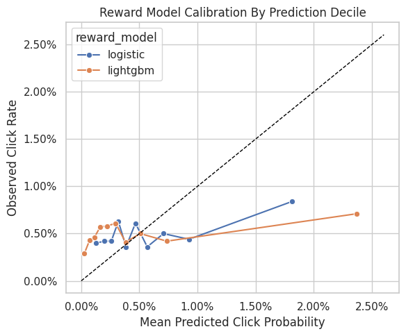
| prediction_bin | mean_prediction | observed_click_rate | rows | reward_model | |
|---|---|---|---|---|---|
| 0 | 0 | 0.001292 | 0.004000 | 10000 | logistic |
| 1 | 1 | 0.001987 | 0.004200 | 10000 | logistic |
| 2 | 2 | 0.002585 | 0.004200 | 10000 | logistic |
| 3 | 3 | 0.003192 | 0.006300 | 10000 | logistic |
| 4 | 4 | 0.003855 | 0.003600 | 10000 | logistic |
| 5 | 5 | 0.004663 | 0.006100 | 10000 | logistic |
| 6 | 6 | 0.005678 | 0.003600 | 10000 | logistic |
| 7 | 7 | 0.007076 | 0.005000 | 10000 | logistic |
| 8 | 8 | 0.009268 | 0.004400 | 10000 | logistic |
| 9 | 9 | 0.018137 | 0.008400 | 10000 | logistic |
| 10 | 0 | 0.000269 | 0.002900 | 10000 | lightgbm |
| 11 | 1 | 0.000718 | 0.004300 | 10000 | lightgbm |
| 12 | 2 | 0.001127 | 0.004600 | 10000 | lightgbm |
| 13 | 3 | 0.001629 | 0.005700 | 10000 | lightgbm |
| 14 | 4 | 0.002242 | 0.005800 | 10000 | lightgbm |
| 15 | 5 | 0.002954 | 0.006100 | 10000 | lightgbm |
| 16 | 6 | 0.003809 | 0.004100 | 10000 | lightgbm |
| 17 | 7 | 0.005085 | 0.005000 | 10000 | lightgbm |
| 18 | 8 | 0.007362 | 0.004200 | 10000 | lightgbm |
| 19 | 9 | 0.023685 | 0.007100 | 10000 | lightgbm |
The reward-model diagnostics show whether predicted click probabilities align with observed clicks. Calibration matters because DR uses these predictions as counterfactual baselines before applying residual correction.
Recreate Evaluation Policies From Notebook 3
This cell rebuilds the same four evaluation policies used in Notebook 3:
uniformexposure_popularityctr_weightedepsilon_greedy_top_ctr
Keeping the policies identical allows us to compare IPS, SNIPS, direct method, and DR estimates without changing the target estimand.
SMOOTHING_ALPHA = 50
train_global_ctr = train_df["click"].mean()

item_stats = (
    train_df.groupby("item_id")
    .agg(train_impressions=("click", "size"), train_clicks=("click", "sum"), train_ctr=("click", "mean"))
    .reindex(action_space, fill_value=0)
    .rename_axis("item_id")
    .reset_index()
)
item_stats["smoothed_ctr"] = (
    item_stats["train_clicks"] + SMOOTHING_ALPHA * train_global_ctr
) / (item_stats["train_impressions"] + SMOOTHING_ALPHA)
item_stats["train_exposure_share"] = item_stats["train_impressions"] / item_stats["train_impressions"].sum()


def normalize_probabilities(values):
    values = np.asarray(values, dtype=float)
    values = np.clip(values, 0, None)
    total = values.sum()
    if total <= 0:
        raise ValueError("Policy scores must have positive total mass.")
    return values / total

uniform_probs = np.full(n_actions, 1 / n_actions)
exposure_popularity_probs = normalize_probabilities(item_stats["train_exposure_share"].to_numpy())
ctr_weighted_probs = normalize_probabilities(item_stats["smoothed_ctr"].to_numpy())

epsilon = 0.15
epsilon_greedy_probs = np.full(n_actions, epsilon / n_actions)
top_ctr_index = int(item_stats["smoothed_ctr"].to_numpy().argmax())
epsilon_greedy_probs[top_ctr_index] += 1 - epsilon

policy_cols = ["uniform", "exposure_popularity", "ctr_weighted", "epsilon_greedy_top_ctr"]
policy_probability_df = pd.DataFrame(
    {
        "item_id": action_space,
        "uniform": uniform_probs,
        "exposure_popularity": exposure_popularity_probs,
        "ctr_weighted": ctr_weighted_probs,
        "epsilon_greedy_top_ctr": epsilon_greedy_probs,
    }
)

policy_probability_df.head()| item_id | uniform | exposure_popularity | ctr_weighted | epsilon_greedy_top_ctr | |
|---|---|---|---|---|---|
| 0 | 0 | 0.029412 | 0.029200 | 0.040498 | 0.004412 |
| 1 | 1 | 0.029412 | 0.027590 | 0.025514 | 0.004412 |
| 2 | 2 | 0.029412 | 0.032070 | 0.036929 | 0.004412 |
| 3 | 3 | 0.029412 | 0.029650 | 0.020188 | 0.004412 |
| 4 | 4 | 0.029412 | 0.028410 | 0.017318 | 0.004412 |
This output is part of the doubly robust off-policy evaluation workflow. Read it as a checkpoint that either verifies the log, defines reusable estimator machinery, or produces a diagnostic that motivates the next OPE step.
Audit Evaluation Policy Probabilities
Before using policy probabilities in an estimator, we check that each policy is valid.
A policy must assign probabilities that sum to 1 and must not assign negative probabilities. In this notebook, every candidate policy also gives every action positive probability, which keeps support diagnostics straightforward.
policy_audit = pd.DataFrame(
    [
        {
            "policy": policy,
            "probability_sum": policy_probability_df[policy].sum(),
            "min_probability": policy_probability_df[policy].min(),
            "max_probability": policy_probability_df[policy].max(),
            "positive_actions": int((policy_probability_df[policy] > 0).sum()),
        }
        for policy in policy_cols
    ]
)

policy_audit| policy | probability_sum | min_probability | max_probability | positive_actions | |
|---|---|---|---|---|---|
| 0 | uniform | 1.000000 | 0.029412 | 0.029412 | 34 |
| 1 | exposure_popularity | 1.000000 | 0.025810 | 0.033300 | 34 |
| 2 | ctr_weighted | 1.000000 | 0.009558 | 0.080613 | 34 |
| 3 | epsilon_greedy_top_ctr | 1.000000 | 0.004412 | 0.854412 | 34 |
This output is part of the doubly robust off-policy evaluation workflow. Read it as a checkpoint that either verifies the log, defines reusable estimator machinery, or produces a diagnostic that motivates the next OPE step.
Create Candidate-Action Feature Frames
The direct method and DR estimator need reward predictions for every candidate action in every evaluation context.
This helper builds a feature frame for all (context, candidate item) pairs in a batch. For each context row, it repeats the context features once per action, attaches candidate item metadata, and selects the affinity score for that candidate item.
Batching keeps memory usage reasonable. The full evaluation split has 100,000 contexts and 34 actions, so scoring everything at once would create 3.4 million rows.
def make_candidate_feature_frame(context_df):
    """Create model features for every candidate action in each context row."""
    n_contexts = len(context_df)
    tiled_actions = np.tile(action_space, n_contexts)

    frame = pd.DataFrame(
        {
            "position": np.repeat(context_df["position"].to_numpy(), n_actions),
            "hour": np.repeat(context_df["hour"].to_numpy(), n_actions),
            "item_id": tiled_actions,
        }
    )

    for col in user_feature_cols:
        frame[col] = np.repeat(context_df[col].to_numpy(), n_actions)

    affinity_matrix = context_df[affinity_cols_by_action].to_numpy()
    frame["selected_affinity"] = affinity_matrix.reshape(-1)

    repeated_item_context = item_context.loc[tiled_actions, item_feature_cols].reset_index(drop=True)
    frame = pd.concat([frame, repeated_item_context], axis=1)

    return frame[feature_cols]

candidate_preview = make_candidate_feature_frame(eval_df.head(2))
candidate_preview| position | hour | item_id | user_feature_0 | user_feature_1 | user_feature_2 | user_feature_3 | item_feature_1 | item_feature_2 | item_feature_3 | selected_affinity | item_feature_0 | |
|---|---|---|---|---|---|---|---|---|---|---|---|---|
| 0 | 2 | 10 | 0 | cef3390ed299c09874189c387777674a | 2d03db5543b14483e52d761760686b64 | 2723d2eb8bba04e0362098011fa3997b | 9bde591ffaab8d54c457448e4dca6f53 | ce58bf66d7e62186e6ce01bafeea9d39 | 7c5498711d69681385d21c0e26923e7e | bbf748c6c978938bc63d432efa60191c | 0.000000 | -0.677183 |
| 1 | 2 | 10 | 1 | cef3390ed299c09874189c387777674a | 2d03db5543b14483e52d761760686b64 | 2723d2eb8bba04e0362098011fa3997b | 9bde591ffaab8d54c457448e4dca6f53 | 3c2985d744e0d57c261abd7e541e4263 | 7c5498711d69681385d21c0e26923e7e | bbf748c6c978938bc63d432efa60191c | 0.000000 | -0.720300 |
| 2 | 2 | 10 | 2 | cef3390ed299c09874189c387777674a | 2d03db5543b14483e52d761760686b64 | 2723d2eb8bba04e0362098011fa3997b | 9bde591ffaab8d54c457448e4dca6f53 | 3c2985d744e0d57c261abd7e541e4263 | 2b851c0a9c4a961da8760d5dc747c5a3 | b61cfaadd526b816e3aeb9b7be4b4759 | 0.000000 | 0.745662 |
| 3 | 2 | 10 | 3 | cef3390ed299c09874189c387777674a | 2d03db5543b14483e52d761760686b64 | 2723d2eb8bba04e0362098011fa3997b | 9bde591ffaab8d54c457448e4dca6f53 | 9874ffb54e9b0a269e29bbb2f5328735 | ce1abd8b5d914ba8fe719b453bc5ba3b | 5bc9c86cd1f08a9991670ea97b34f86d | 0.000000 | -0.698741 |
| 4 | 2 | 10 | 4 | cef3390ed299c09874189c387777674a | 2d03db5543b14483e52d761760686b64 | 2723d2eb8bba04e0362098011fa3997b | 9bde591ffaab8d54c457448e4dca6f53 | 01fe2f187e459e6ada960671d2942dfe | b4b5879029fb5f64eeec63cf4f73ef0e | b61cfaadd526b816e3aeb9b7be4b4759 | 0.000000 | 1.651109 |
| 5 | 2 | 10 | 5 | cef3390ed299c09874189c387777674a | 2d03db5543b14483e52d761760686b64 | 2723d2eb8bba04e0362098011fa3997b | 9bde591ffaab8d54c457448e4dca6f53 | 01fe2f187e459e6ada960671d2942dfe | c43671ed6855a6fe2e2a6030cba64366 | bbf748c6c978938bc63d432efa60191c | 0.000000 | 0.142031 |
| 6 | 2 | 10 | 6 | cef3390ed299c09874189c387777674a | 2d03db5543b14483e52d761760686b64 | 2723d2eb8bba04e0362098011fa3997b | 9bde591ffaab8d54c457448e4dca6f53 | ce58bf66d7e62186e6ce01bafeea9d39 | 7082af732502f0981a9fe77d7ba1ae8a | b61cfaadd526b816e3aeb9b7be4b4759 | 0.000000 | 1.651109 |
| 7 | 2 | 10 | 7 | cef3390ed299c09874189c387777674a | 2d03db5543b14483e52d761760686b64 | 2723d2eb8bba04e0362098011fa3997b | 9bde591ffaab8d54c457448e4dca6f53 | 01fe2f187e459e6ada960671d2942dfe | 2b851c0a9c4a961da8760d5dc747c5a3 | b61cfaadd526b816e3aeb9b7be4b4759 | 0.000000 | 2.858372 |
| 8 | 2 | 10 | 8 | cef3390ed299c09874189c387777674a | 2d03db5543b14483e52d761760686b64 | 2723d2eb8bba04e0362098011fa3997b | 9bde591ffaab8d54c457448e4dca6f53 | 01fe2f187e459e6ada960671d2942dfe | d7f03898d040700d6e1810d21e669958 | b61cfaadd526b816e3aeb9b7be4b4759 | 0.000000 | 1.349294 |
| 9 | 2 | 10 | 9 | cef3390ed299c09874189c387777674a | 2d03db5543b14483e52d761760686b64 | 2723d2eb8bba04e0362098011fa3997b | 9bde591ffaab8d54c457448e4dca6f53 | 9874ffb54e9b0a269e29bbb2f5328735 | 2b851c0a9c4a961da8760d5dc747c5a3 | b61cfaadd526b816e3aeb9b7be4b4759 | 0.000000 | 1.198386 |
| 10 | 2 | 10 | 10 | cef3390ed299c09874189c387777674a | 2d03db5543b14483e52d761760686b64 | 2723d2eb8bba04e0362098011fa3997b | 9bde591ffaab8d54c457448e4dca6f53 | 9874ffb54e9b0a269e29bbb2f5328735 | 2b851c0a9c4a961da8760d5dc747c5a3 | b61cfaadd526b816e3aeb9b7be4b4759 | 0.000000 | 1.586435 |
| 11 | 2 | 10 | 11 | cef3390ed299c09874189c387777674a | 2d03db5543b14483e52d761760686b64 | 2723d2eb8bba04e0362098011fa3997b | 9bde591ffaab8d54c457448e4dca6f53 | ce58bf66d7e62186e6ce01bafeea9d39 | eddad9910a6d2f61905f408d4df575c5 | de8b129010093b09b24a05592bfd8843 | 0.000000 | 0.443847 |
| 12 | 2 | 10 | 12 | cef3390ed299c09874189c387777674a | 2d03db5543b14483e52d761760686b64 | 2723d2eb8bba04e0362098011fa3997b | 9bde591ffaab8d54c457448e4dca6f53 | ce58bf66d7e62186e6ce01bafeea9d39 | 697cbf60c7c4b8569c149721231538c3 | b61cfaadd526b816e3aeb9b7be4b4759 | 0.000000 | 1.198386 |
| 13 | 2 | 10 | 13 | cef3390ed299c09874189c387777674a | 2d03db5543b14483e52d761760686b64 | 2723d2eb8bba04e0362098011fa3997b | 9bde591ffaab8d54c457448e4dca6f53 | 9874ffb54e9b0a269e29bbb2f5328735 | 697cbf60c7c4b8569c149721231538c3 | b61cfaadd526b816e3aeb9b7be4b4759 | 0.000000 | 0.616313 |
| 14 | 2 | 10 | 14 | cef3390ed299c09874189c387777674a | 2d03db5543b14483e52d761760686b64 | 2723d2eb8bba04e0362098011fa3997b | 9bde591ffaab8d54c457448e4dca6f53 | 9874ffb54e9b0a269e29bbb2f5328735 | 3f1feafd79578bedf199c459fecc378b | bbf748c6c978938bc63d432efa60191c | 0.000000 | -1.000557 |
| 15 | 2 | 10 | 15 | cef3390ed299c09874189c387777674a | 2d03db5543b14483e52d761760686b64 | 2723d2eb8bba04e0362098011fa3997b | 9bde591ffaab8d54c457448e4dca6f53 | ce58bf66d7e62186e6ce01bafeea9d39 | 9f9ff361c09f765650f1c43ef7adac86 | 5bc9c86cd1f08a9991670ea97b34f86d | 0.000000 | -0.375367 |
| 16 | 2 | 10 | 16 | cef3390ed299c09874189c387777674a | 2d03db5543b14483e52d761760686b64 | 2723d2eb8bba04e0362098011fa3997b | 9bde591ffaab8d54c457448e4dca6f53 | ce58bf66d7e62186e6ce01bafeea9d39 | 5d5dd3635cb3f84d3a70f5874a132d44 | 5bc9c86cd1f08a9991670ea97b34f86d | 0.000000 | -0.590950 |
| 17 | 2 | 10 | 17 | cef3390ed299c09874189c387777674a | 2d03db5543b14483e52d761760686b64 | 2723d2eb8bba04e0362098011fa3997b | 9bde591ffaab8d54c457448e4dca6f53 | 9874ffb54e9b0a269e29bbb2f5328735 | 5d5dd3635cb3f84d3a70f5874a132d44 | 5bc9c86cd1f08a9991670ea97b34f86d | 0.000000 | -0.698741 |
| 18 | 2 | 10 | 18 | cef3390ed299c09874189c387777674a | 2d03db5543b14483e52d761760686b64 | 2723d2eb8bba04e0362098011fa3997b | 9bde591ffaab8d54c457448e4dca6f53 | 3c2985d744e0d57c261abd7e541e4263 | 5d5dd3635cb3f84d3a70f5874a132d44 | 5bc9c86cd1f08a9991670ea97b34f86d | 0.000000 | -0.914324 |
| 19 | 2 | 10 | 19 | cef3390ed299c09874189c387777674a | 2d03db5543b14483e52d761760686b64 | 2723d2eb8bba04e0362098011fa3997b | 9bde591ffaab8d54c457448e4dca6f53 | 3c2985d744e0d57c261abd7e541e4263 | 5d5dd3635cb3f84d3a70f5874a132d44 | 5bc9c86cd1f08a9991670ea97b34f86d | 0.000000 | -0.763416 |
| 20 | 2 | 10 | 20 | cef3390ed299c09874189c387777674a | 2d03db5543b14483e52d761760686b64 | 2723d2eb8bba04e0362098011fa3997b | 9bde591ffaab8d54c457448e4dca6f53 | 3c2985d744e0d57c261abd7e541e4263 | 5d5dd3635cb3f84d3a70f5874a132d44 | 5bc9c86cd1f08a9991670ea97b34f86d | 0.000000 | -0.612508 |
| 21 | 2 | 10 | 21 | cef3390ed299c09874189c387777674a | 2d03db5543b14483e52d761760686b64 | 2723d2eb8bba04e0362098011fa3997b | 9bde591ffaab8d54c457448e4dca6f53 | 9874ffb54e9b0a269e29bbb2f5328735 | ce1abd8b5d914ba8fe719b453bc5ba3b | 5bc9c86cd1f08a9991670ea97b34f86d | 0.000000 | -0.698741 |
| 22 | 2 | 10 | 22 | cef3390ed299c09874189c387777674a | 2d03db5543b14483e52d761760686b64 | 2723d2eb8bba04e0362098011fa3997b | 9bde591ffaab8d54c457448e4dca6f53 | 61c5d8c2524684aa047e15e172c7e92f | 7c5498711d69681385d21c0e26923e7e | bbf748c6c978938bc63d432efa60191c | 0.000000 | -0.698741 |
| 23 | 2 | 10 | 23 | cef3390ed299c09874189c387777674a | 2d03db5543b14483e52d761760686b64 | 2723d2eb8bba04e0362098011fa3997b | 9bde591ffaab8d54c457448e4dca6f53 | 55fe518d85813954c7d9b8a875ff2453 | cc75031396a5aa830885915aa93f49d0 | b61cfaadd526b816e3aeb9b7be4b4759 | 0.000000 | -0.569392 |
| 24 | 2 | 10 | 24 | cef3390ed299c09874189c387777674a | 2d03db5543b14483e52d761760686b64 | 2723d2eb8bba04e0362098011fa3997b | 9bde591ffaab8d54c457448e4dca6f53 | e95f0d1a3591e01d7ed3f0710424e84d | d7f03898d040700d6e1810d21e669958 | b61cfaadd526b816e3aeb9b7be4b4759 | 0.000000 | 0.422288 |
| 25 | 2 | 10 | 25 | cef3390ed299c09874189c387777674a | 2d03db5543b14483e52d761760686b64 | 2723d2eb8bba04e0362098011fa3997b | 9bde591ffaab8d54c457448e4dca6f53 | 9874ffb54e9b0a269e29bbb2f5328735 | 7c5498711d69681385d21c0e26923e7e | bbf748c6c978938bc63d432efa60191c | 0.000000 | -0.461600 |
| 26 | 2 | 10 | 26 | cef3390ed299c09874189c387777674a | 2d03db5543b14483e52d761760686b64 | 2723d2eb8bba04e0362098011fa3997b | 9bde591ffaab8d54c457448e4dca6f53 | 3c2985d744e0d57c261abd7e541e4263 | a86ead010f033dbc2854c6a46f4fe7a7 | b61cfaadd526b816e3aeb9b7be4b4759 | 0.000000 | 0.896570 |
| 27 | 2 | 10 | 27 | cef3390ed299c09874189c387777674a | 2d03db5543b14483e52d761760686b64 | 2723d2eb8bba04e0362098011fa3997b | 9bde591ffaab8d54c457448e4dca6f53 | 61c5d8c2524684aa047e15e172c7e92f | 5d5dd3635cb3f84d3a70f5874a132d44 | 5bc9c86cd1f08a9991670ea97b34f86d | 0.000000 | -0.849649 |
| 28 | 2 | 10 | 28 | cef3390ed299c09874189c387777674a | 2d03db5543b14483e52d761760686b64 | 2723d2eb8bba04e0362098011fa3997b | 9bde591ffaab8d54c457448e4dca6f53 | 61c5d8c2524684aa047e15e172c7e92f | b726ac74a20945400f27294febd4ab55 | 5bc9c86cd1f08a9991670ea97b34f86d | 0.000000 | -1.065232 |
| 29 | 2 | 10 | 29 | cef3390ed299c09874189c387777674a | 2d03db5543b14483e52d761760686b64 | 2723d2eb8bba04e0362098011fa3997b | 9bde591ffaab8d54c457448e4dca6f53 | 61c5d8c2524684aa047e15e172c7e92f | 7c63a6aa72e655abd1787c2e64385e6f | bbf748c6c978938bc63d432efa60191c | 0.000000 | -0.849649 |
| 30 | 2 | 10 | 30 | cef3390ed299c09874189c387777674a | 2d03db5543b14483e52d761760686b64 | 2723d2eb8bba04e0362098011fa3997b | 9bde591ffaab8d54c457448e4dca6f53 | 61c5d8c2524684aa047e15e172c7e92f | 3f1feafd79578bedf199c459fecc378b | bbf748c6c978938bc63d432efa60191c | 0.000000 | -0.914324 |
| 31 | 2 | 10 | 31 | cef3390ed299c09874189c387777674a | 2d03db5543b14483e52d761760686b64 | 2723d2eb8bba04e0362098011fa3997b | 9bde591ffaab8d54c457448e4dca6f53 | 55fe518d85813954c7d9b8a875ff2453 | 7c63a6aa72e655abd1787c2e64385e6f | bbf748c6c978938bc63d432efa60191c | 0.000000 | -0.461600 |
| 32 | 2 | 10 | 32 | cef3390ed299c09874189c387777674a | 2d03db5543b14483e52d761760686b64 | 2723d2eb8bba04e0362098011fa3997b | 9bde591ffaab8d54c457448e4dca6f53 | e95f0d1a3591e01d7ed3f0710424e84d | b726ac74a20945400f27294febd4ab55 | 5bc9c86cd1f08a9991670ea97b34f86d | 0.000000 | -0.526275 |
| 33 | 2 | 10 | 33 | cef3390ed299c09874189c387777674a | 2d03db5543b14483e52d761760686b64 | 2723d2eb8bba04e0362098011fa3997b | 9bde591ffaab8d54c457448e4dca6f53 | e95f0d1a3591e01d7ed3f0710424e84d | 7c5498711d69681385d21c0e26923e7e | bbf748c6c978938bc63d432efa60191c | 0.000000 | -0.612508 |
| 34 | 2 | 10 | 0 | cef3390ed299c09874189c387777674a | 03a5648a76832f83c859d46bc06cb64a | 9b2d331c329ceb74d3dcfb48d8798c78 | f97571b9c14a786aab269f0b427d2a85 | ce58bf66d7e62186e6ce01bafeea9d39 | 7c5498711d69681385d21c0e26923e7e | bbf748c6c978938bc63d432efa60191c | 0.000000 | -0.677183 |
| 35 | 2 | 10 | 1 | cef3390ed299c09874189c387777674a | 03a5648a76832f83c859d46bc06cb64a | 9b2d331c329ceb74d3dcfb48d8798c78 | f97571b9c14a786aab269f0b427d2a85 | 3c2985d744e0d57c261abd7e541e4263 | 7c5498711d69681385d21c0e26923e7e | bbf748c6c978938bc63d432efa60191c | 0.000000 | -0.720300 |
| 36 | 2 | 10 | 2 | cef3390ed299c09874189c387777674a | 03a5648a76832f83c859d46bc06cb64a | 9b2d331c329ceb74d3dcfb48d8798c78 | f97571b9c14a786aab269f0b427d2a85 | 3c2985d744e0d57c261abd7e541e4263 | 2b851c0a9c4a961da8760d5dc747c5a3 | b61cfaadd526b816e3aeb9b7be4b4759 | 0.000000 | 0.745662 |
| 37 | 2 | 10 | 3 | cef3390ed299c09874189c387777674a | 03a5648a76832f83c859d46bc06cb64a | 9b2d331c329ceb74d3dcfb48d8798c78 | f97571b9c14a786aab269f0b427d2a85 | 9874ffb54e9b0a269e29bbb2f5328735 | ce1abd8b5d914ba8fe719b453bc5ba3b | 5bc9c86cd1f08a9991670ea97b34f86d | 0.000000 | -0.698741 |
| 38 | 2 | 10 | 4 | cef3390ed299c09874189c387777674a | 03a5648a76832f83c859d46bc06cb64a | 9b2d331c329ceb74d3dcfb48d8798c78 | f97571b9c14a786aab269f0b427d2a85 | 01fe2f187e459e6ada960671d2942dfe | b4b5879029fb5f64eeec63cf4f73ef0e | b61cfaadd526b816e3aeb9b7be4b4759 | 0.000000 | 1.651109 |
| 39 | 2 | 10 | 5 | cef3390ed299c09874189c387777674a | 03a5648a76832f83c859d46bc06cb64a | 9b2d331c329ceb74d3dcfb48d8798c78 | f97571b9c14a786aab269f0b427d2a85 | 01fe2f187e459e6ada960671d2942dfe | c43671ed6855a6fe2e2a6030cba64366 | bbf748c6c978938bc63d432efa60191c | 0.000000 | 0.142031 |
| 40 | 2 | 10 | 6 | cef3390ed299c09874189c387777674a | 03a5648a76832f83c859d46bc06cb64a | 9b2d331c329ceb74d3dcfb48d8798c78 | f97571b9c14a786aab269f0b427d2a85 | ce58bf66d7e62186e6ce01bafeea9d39 | 7082af732502f0981a9fe77d7ba1ae8a | b61cfaadd526b816e3aeb9b7be4b4759 | 0.000000 | 1.651109 |
| 41 | 2 | 10 | 7 | cef3390ed299c09874189c387777674a | 03a5648a76832f83c859d46bc06cb64a | 9b2d331c329ceb74d3dcfb48d8798c78 | f97571b9c14a786aab269f0b427d2a85 | 01fe2f187e459e6ada960671d2942dfe | 2b851c0a9c4a961da8760d5dc747c5a3 | b61cfaadd526b816e3aeb9b7be4b4759 | 0.000000 | 2.858372 |
| 42 | 2 | 10 | 8 | cef3390ed299c09874189c387777674a | 03a5648a76832f83c859d46bc06cb64a | 9b2d331c329ceb74d3dcfb48d8798c78 | f97571b9c14a786aab269f0b427d2a85 | 01fe2f187e459e6ada960671d2942dfe | d7f03898d040700d6e1810d21e669958 | b61cfaadd526b816e3aeb9b7be4b4759 | 0.000000 | 1.349294 |
| 43 | 2 | 10 | 9 | cef3390ed299c09874189c387777674a | 03a5648a76832f83c859d46bc06cb64a | 9b2d331c329ceb74d3dcfb48d8798c78 | f97571b9c14a786aab269f0b427d2a85 | 9874ffb54e9b0a269e29bbb2f5328735 | 2b851c0a9c4a961da8760d5dc747c5a3 | b61cfaadd526b816e3aeb9b7be4b4759 | 0.000000 | 1.198386 |
| 44 | 2 | 10 | 10 | cef3390ed299c09874189c387777674a | 03a5648a76832f83c859d46bc06cb64a | 9b2d331c329ceb74d3dcfb48d8798c78 | f97571b9c14a786aab269f0b427d2a85 | 9874ffb54e9b0a269e29bbb2f5328735 | 2b851c0a9c4a961da8760d5dc747c5a3 | b61cfaadd526b816e3aeb9b7be4b4759 | 0.000000 | 1.586435 |
| 45 | 2 | 10 | 11 | cef3390ed299c09874189c387777674a | 03a5648a76832f83c859d46bc06cb64a | 9b2d331c329ceb74d3dcfb48d8798c78 | f97571b9c14a786aab269f0b427d2a85 | ce58bf66d7e62186e6ce01bafeea9d39 | eddad9910a6d2f61905f408d4df575c5 | de8b129010093b09b24a05592bfd8843 | 0.000000 | 0.443847 |
| 46 | 2 | 10 | 12 | cef3390ed299c09874189c387777674a | 03a5648a76832f83c859d46bc06cb64a | 9b2d331c329ceb74d3dcfb48d8798c78 | f97571b9c14a786aab269f0b427d2a85 | ce58bf66d7e62186e6ce01bafeea9d39 | 697cbf60c7c4b8569c149721231538c3 | b61cfaadd526b816e3aeb9b7be4b4759 | 0.000000 | 1.198386 |
| 47 | 2 | 10 | 13 | cef3390ed299c09874189c387777674a | 03a5648a76832f83c859d46bc06cb64a | 9b2d331c329ceb74d3dcfb48d8798c78 | f97571b9c14a786aab269f0b427d2a85 | 9874ffb54e9b0a269e29bbb2f5328735 | 697cbf60c7c4b8569c149721231538c3 | b61cfaadd526b816e3aeb9b7be4b4759 | 0.000000 | 0.616313 |
| 48 | 2 | 10 | 14 | cef3390ed299c09874189c387777674a | 03a5648a76832f83c859d46bc06cb64a | 9b2d331c329ceb74d3dcfb48d8798c78 | f97571b9c14a786aab269f0b427d2a85 | 9874ffb54e9b0a269e29bbb2f5328735 | 3f1feafd79578bedf199c459fecc378b | bbf748c6c978938bc63d432efa60191c | 0.000000 | -1.000557 |
| 49 | 2 | 10 | 15 | cef3390ed299c09874189c387777674a | 03a5648a76832f83c859d46bc06cb64a | 9b2d331c329ceb74d3dcfb48d8798c78 | f97571b9c14a786aab269f0b427d2a85 | ce58bf66d7e62186e6ce01bafeea9d39 | 9f9ff361c09f765650f1c43ef7adac86 | 5bc9c86cd1f08a9991670ea97b34f86d | 0.000000 | -0.375367 |
| 50 | 2 | 10 | 16 | cef3390ed299c09874189c387777674a | 03a5648a76832f83c859d46bc06cb64a | 9b2d331c329ceb74d3dcfb48d8798c78 | f97571b9c14a786aab269f0b427d2a85 | ce58bf66d7e62186e6ce01bafeea9d39 | 5d5dd3635cb3f84d3a70f5874a132d44 | 5bc9c86cd1f08a9991670ea97b34f86d | 0.000000 | -0.590950 |
| 51 | 2 | 10 | 17 | cef3390ed299c09874189c387777674a | 03a5648a76832f83c859d46bc06cb64a | 9b2d331c329ceb74d3dcfb48d8798c78 | f97571b9c14a786aab269f0b427d2a85 | 9874ffb54e9b0a269e29bbb2f5328735 | 5d5dd3635cb3f84d3a70f5874a132d44 | 5bc9c86cd1f08a9991670ea97b34f86d | 0.000000 | -0.698741 |
| 52 | 2 | 10 | 18 | cef3390ed299c09874189c387777674a | 03a5648a76832f83c859d46bc06cb64a | 9b2d331c329ceb74d3dcfb48d8798c78 | f97571b9c14a786aab269f0b427d2a85 | 3c2985d744e0d57c261abd7e541e4263 | 5d5dd3635cb3f84d3a70f5874a132d44 | 5bc9c86cd1f08a9991670ea97b34f86d | 0.000000 | -0.914324 |
| 53 | 2 | 10 | 19 | cef3390ed299c09874189c387777674a | 03a5648a76832f83c859d46bc06cb64a | 9b2d331c329ceb74d3dcfb48d8798c78 | f97571b9c14a786aab269f0b427d2a85 | 3c2985d744e0d57c261abd7e541e4263 | 5d5dd3635cb3f84d3a70f5874a132d44 | 5bc9c86cd1f08a9991670ea97b34f86d | 0.000000 | -0.763416 |
| 54 | 2 | 10 | 20 | cef3390ed299c09874189c387777674a | 03a5648a76832f83c859d46bc06cb64a | 9b2d331c329ceb74d3dcfb48d8798c78 | f97571b9c14a786aab269f0b427d2a85 | 3c2985d744e0d57c261abd7e541e4263 | 5d5dd3635cb3f84d3a70f5874a132d44 | 5bc9c86cd1f08a9991670ea97b34f86d | 0.000000 | -0.612508 |
| 55 | 2 | 10 | 21 | cef3390ed299c09874189c387777674a | 03a5648a76832f83c859d46bc06cb64a | 9b2d331c329ceb74d3dcfb48d8798c78 | f97571b9c14a786aab269f0b427d2a85 | 9874ffb54e9b0a269e29bbb2f5328735 | ce1abd8b5d914ba8fe719b453bc5ba3b | 5bc9c86cd1f08a9991670ea97b34f86d | 0.000000 | -0.698741 |
| 56 | 2 | 10 | 22 | cef3390ed299c09874189c387777674a | 03a5648a76832f83c859d46bc06cb64a | 9b2d331c329ceb74d3dcfb48d8798c78 | f97571b9c14a786aab269f0b427d2a85 | 61c5d8c2524684aa047e15e172c7e92f | 7c5498711d69681385d21c0e26923e7e | bbf748c6c978938bc63d432efa60191c | 0.000000 | -0.698741 |
| 57 | 2 | 10 | 23 | cef3390ed299c09874189c387777674a | 03a5648a76832f83c859d46bc06cb64a | 9b2d331c329ceb74d3dcfb48d8798c78 | f97571b9c14a786aab269f0b427d2a85 | 55fe518d85813954c7d9b8a875ff2453 | cc75031396a5aa830885915aa93f49d0 | b61cfaadd526b816e3aeb9b7be4b4759 | 0.000000 | -0.569392 |
| 58 | 2 | 10 | 24 | cef3390ed299c09874189c387777674a | 03a5648a76832f83c859d46bc06cb64a | 9b2d331c329ceb74d3dcfb48d8798c78 | f97571b9c14a786aab269f0b427d2a85 | e95f0d1a3591e01d7ed3f0710424e84d | d7f03898d040700d6e1810d21e669958 | b61cfaadd526b816e3aeb9b7be4b4759 | 0.000000 | 0.422288 |
| 59 | 2 | 10 | 25 | cef3390ed299c09874189c387777674a | 03a5648a76832f83c859d46bc06cb64a | 9b2d331c329ceb74d3dcfb48d8798c78 | f97571b9c14a786aab269f0b427d2a85 | 9874ffb54e9b0a269e29bbb2f5328735 | 7c5498711d69681385d21c0e26923e7e | bbf748c6c978938bc63d432efa60191c | 0.000000 | -0.461600 |
| 60 | 2 | 10 | 26 | cef3390ed299c09874189c387777674a | 03a5648a76832f83c859d46bc06cb64a | 9b2d331c329ceb74d3dcfb48d8798c78 | f97571b9c14a786aab269f0b427d2a85 | 3c2985d744e0d57c261abd7e541e4263 | a86ead010f033dbc2854c6a46f4fe7a7 | b61cfaadd526b816e3aeb9b7be4b4759 | 0.000000 | 0.896570 |
| 61 | 2 | 10 | 27 | cef3390ed299c09874189c387777674a | 03a5648a76832f83c859d46bc06cb64a | 9b2d331c329ceb74d3dcfb48d8798c78 | f97571b9c14a786aab269f0b427d2a85 | 61c5d8c2524684aa047e15e172c7e92f | 5d5dd3635cb3f84d3a70f5874a132d44 | 5bc9c86cd1f08a9991670ea97b34f86d | 0.000000 | -0.849649 |
| 62 | 2 | 10 | 28 | cef3390ed299c09874189c387777674a | 03a5648a76832f83c859d46bc06cb64a | 9b2d331c329ceb74d3dcfb48d8798c78 | f97571b9c14a786aab269f0b427d2a85 | 61c5d8c2524684aa047e15e172c7e92f | b726ac74a20945400f27294febd4ab55 | 5bc9c86cd1f08a9991670ea97b34f86d | 0.000000 | -1.065232 |
| 63 | 2 | 10 | 29 | cef3390ed299c09874189c387777674a | 03a5648a76832f83c859d46bc06cb64a | 9b2d331c329ceb74d3dcfb48d8798c78 | f97571b9c14a786aab269f0b427d2a85 | 61c5d8c2524684aa047e15e172c7e92f | 7c63a6aa72e655abd1787c2e64385e6f | bbf748c6c978938bc63d432efa60191c | 0.000000 | -0.849649 |
| 64 | 2 | 10 | 30 | cef3390ed299c09874189c387777674a | 03a5648a76832f83c859d46bc06cb64a | 9b2d331c329ceb74d3dcfb48d8798c78 | f97571b9c14a786aab269f0b427d2a85 | 61c5d8c2524684aa047e15e172c7e92f | 3f1feafd79578bedf199c459fecc378b | bbf748c6c978938bc63d432efa60191c | 0.000000 | -0.914324 |
| 65 | 2 | 10 | 31 | cef3390ed299c09874189c387777674a | 03a5648a76832f83c859d46bc06cb64a | 9b2d331c329ceb74d3dcfb48d8798c78 | f97571b9c14a786aab269f0b427d2a85 | 55fe518d85813954c7d9b8a875ff2453 | 7c63a6aa72e655abd1787c2e64385e6f | bbf748c6c978938bc63d432efa60191c | 0.000000 | -0.461600 |
| 66 | 2 | 10 | 32 | cef3390ed299c09874189c387777674a | 03a5648a76832f83c859d46bc06cb64a | 9b2d331c329ceb74d3dcfb48d8798c78 | f97571b9c14a786aab269f0b427d2a85 | e95f0d1a3591e01d7ed3f0710424e84d | b726ac74a20945400f27294febd4ab55 | 5bc9c86cd1f08a9991670ea97b34f86d | 0.000000 | -0.526275 |
| 67 | 2 | 10 | 33 | cef3390ed299c09874189c387777674a | 03a5648a76832f83c859d46bc06cb64a | 9b2d331c329ceb74d3dcfb48d8798c78 | f97571b9c14a786aab269f0b427d2a85 | e95f0d1a3591e01d7ed3f0710424e84d | 7c5498711d69681385d21c0e26923e7e | bbf748c6c978938bc63d432efa60191c | 0.000000 | -0.612508 |
These feature-building cells define the context used by reward models. Reward models need both user context and candidate item context so they can predict counterfactual rewards for actions that were not logged.
Compute Direct-Method Components In Batches
This helper scores every evaluation context against every candidate item for one reward model.
For each context, it computes:
sum_a pi_e(a|x) * q_hat(x, a)
Because our evaluation policies are context-free, the policy probabilities do not vary by row. The reward predictions still vary by row because user features, position, hour, and selected affinity vary by context.
def compute_direct_components(model, contexts_df, batch_size=10_000):
    """Return one direct-method component per context and policy."""
    policy_probability_matrix = policy_probability_df[policy_cols].to_numpy()
    component_batches = []

    for start in range(0, len(contexts_df), batch_size):
        context_batch = contexts_df.iloc[start : start + batch_size]
        candidate_features = make_candidate_feature_frame(context_batch)
        q_hat = model.predict_proba(candidate_features)[:, 1].reshape(len(context_batch), n_actions)
        direct_components = q_hat @ policy_probability_matrix
        component_batches.append(direct_components)

    components = np.vstack(component_batches)
    return pd.DataFrame(components, columns=policy_cols, index=contexts_df.index)
These cells score candidate actions under the reward model, which is what lets the direct method estimate values for policies that choose actions different from the logged one. This is the model-based complement to importance weighting.
Score Logged Actions And Candidate Actions
This cell produces the two reward-model prediction objects needed for DR:
q_hat_logged: predicted click probability for the item that was actually loggeddirect_components: expected predicted reward under each evaluation policy for each context
The direct components are the model-based policy values before residual correction.
q_logged_by_model = {}
direct_components_by_model = {}

for model_name, model in reward_models.items():
    q_logged_by_model[model_name] = model.predict_proba(X_eval_logged)[:, 1]
    direct_components_by_model[model_name] = compute_direct_components(model, eval_df, batch_size=10_000)

pd.DataFrame(
    {
        "reward_model": list(q_logged_by_model),
        "mean_q_logged": [pred.mean() for pred in q_logged_by_model.values()],
        "direct_component_rows": [len(direct_components_by_model[name]) for name in q_logged_by_model],
    }
)| reward_model | mean_q_logged | direct_component_rows | |
|---|---|---|---|
| 0 | logistic | 0.005774 | 100000 |
| 1 | lightgbm | 0.004888 | 100000 |
These cells score candidate actions under the reward model, which is what lets the direct method estimate values for policies that choose actions different from the logged one. This is the model-based complement to importance weighting.
Attach Evaluation Policy Weights
This cell computes pi_e(A|X) / pi_b(A|X) for the logged action under each evaluation policy.
These are the same importance weights used in Notebook 3. In the doubly robust estimator, the weights multiply the reward-model residual Y - q_hat(X, A) rather than the raw reward Y.
eval_scored = eval_df[["timestamp", "item_id", "position", "click", "propensity_score"]].copy()

for policy in policy_cols:
    probability_map = policy_probability_df.set_index("item_id")[policy]
    eval_scored[f"pi_e_{policy}"] = eval_scored["item_id"].map(probability_map)
    eval_scored[f"w_{policy}"] = eval_scored[f"pi_e_{policy}"] / eval_scored["propensity_score"]

weight_check = pd.DataFrame(
    [
        {
            "policy": policy,
            "mean_weight": eval_scored[f"w_{policy}"].mean(),
            "max_weight": eval_scored[f"w_{policy}"].max(),
            "p99_weight": np.percentile(eval_scored[f"w_{policy}"], 99),
        }
        for policy in policy_cols
    ]
)

weight_check| policy | mean_weight | max_weight | p99_weight | |
|---|---|---|---|---|
| 0 | uniform | 1.000000 | 1.000000 | 1.000000 |
| 1 | exposure_popularity | 1.000591 | 1.132200 | 1.132200 |
| 2 | ctr_weighted | 0.996987 | 2.740842 | 2.740842 |
| 3 | epsilon_greedy_top_ctr | 1.001105 | 29.050000 | 29.050000 |
Attaching evaluation-policy probabilities to logged rows creates the numerator of the importance weight. Once this is joined to the behavior propensity, IPS and SNIPS can estimate each policy’s value.
Define OPE Estimator Helpers
This cell defines helper functions for IPS, SNIPS, direct method, and doubly robust estimation.
Each estimator returns an estimate, approximate standard error, confidence interval, and weight diagnostics where relevant. The confidence intervals use large-sample standard errors. They are useful for comparison, but later production work would likely use richer bootstrap or repeated-split diagnostics.
def effective_sample_size(weights):
    weights = np.asarray(weights, dtype=float)
    return weights.sum() ** 2 / np.square(weights).sum()


def summarize_signal(signal):
    signal = np.asarray(signal, dtype=float)
    estimate = signal.mean()
    se = signal.std(ddof=1) / np.sqrt(len(signal))
    return estimate, se, estimate - 1.96 * se, estimate + 1.96 * se


def estimate_ips_snips(reward, weight):
    reward = np.asarray(reward, dtype=float)
    weight = np.asarray(weight, dtype=float)
    ips_signal = weight * reward
    ips, ips_se, ips_lower, ips_upper = summarize_signal(ips_signal)

    snips = ips_signal.sum() / weight.sum()
    snips_influence = weight * (reward - snips) / weight.mean()
    snips_se = snips_influence.std(ddof=1) / np.sqrt(len(snips_influence))

    return {
        "ips": (ips, ips_se, ips_lower, ips_upper),
        "snips": (snips, snips_se, snips - 1.96 * snips_se, snips + 1.96 * snips_se),
        "ess_share": effective_sample_size(weight) / len(weight),
        "mean_weight": weight.mean(),
        "max_weight": weight.max(),
    }


def estimate_dm_dr(reward, weight, q_logged, direct_component):
    reward = np.asarray(reward, dtype=float)
    weight = np.asarray(weight, dtype=float)
    q_logged = np.asarray(q_logged, dtype=float)
    direct_component = np.asarray(direct_component, dtype=float)

    dm, dm_se, dm_lower, dm_upper = summarize_signal(direct_component)
    dr_signal = direct_component + weight * (reward - q_logged)
    dr, dr_se, dr_lower, dr_upper = summarize_signal(dr_signal)

    correction = dr_signal - direct_component
    return {
        "dm": (dm, dm_se, dm_lower, dm_upper),
        "dr": (dr, dr_se, dr_lower, dr_upper),
        "mean_abs_correction": np.abs(correction).mean(),
        "mean_correction": correction.mean(),
    }
The helper functions encode the estimator formulas and diagnostics used repeatedly in the notebook. Defining them once keeps the later policy comparisons consistent and easier to audit.
Estimate IPS, SNIPS, Direct Method, And DR
This cell computes the main OPE result table.
For each policy, IPS and SNIPS depend only on propensities and observed rewards. Direct method and DR are computed separately for each reward model. The DR estimate uses the reward model prediction plus an importance-weighted residual correction.
result_rows = []
reward = eval_scored["click"].to_numpy()

for policy in policy_cols:
    weight = eval_scored[f"w_{policy}"].to_numpy()
    ips_snips = estimate_ips_snips(reward, weight)

    for estimator_name, values in [("IPS", ips_snips["ips"]), ("SNIPS", ips_snips["snips"] )]:
        estimate, se, lower, upper = values
        result_rows.append(
            {
                "policy": policy,
                "estimator": estimator_name,
                "reward_model": "none",
                "estimate": estimate,
                "se": se,
                "ci_95_lower": lower,
                "ci_95_upper": upper,
                "ess_share": ips_snips["ess_share"],
                "mean_weight": ips_snips["mean_weight"],
                "max_weight": ips_snips["max_weight"],
                "mean_abs_correction": np.nan,
                "mean_correction": np.nan,
            }
        )

    for model_name in reward_models:
        dm_dr = estimate_dm_dr(
            reward=reward,
            weight=weight,
            q_logged=q_logged_by_model[model_name],
            direct_component=direct_components_by_model[model_name][policy],
        )
        for estimator_name, values in [("DM", dm_dr["dm"]), ("DR", dm_dr["dr"] )]:
            estimate, se, lower, upper = values
            result_rows.append(
                {
                    "policy": policy,
                    "estimator": estimator_name,
                    "reward_model": model_name,
                    "estimate": estimate,
                    "se": se,
                    "ci_95_lower": lower,
                    "ci_95_upper": upper,
                    "ess_share": ips_snips["ess_share"],
                    "mean_weight": ips_snips["mean_weight"],
                    "max_weight": ips_snips["max_weight"],
                    "mean_abs_correction": dm_dr["mean_abs_correction"],
                    "mean_correction": dm_dr["mean_correction"],
                }
            )

all_estimates = pd.DataFrame(result_rows)
all_estimates.head(12)| policy | estimator | reward_model | estimate | se | ci_95_lower | ci_95_upper | ess_share | mean_weight | max_weight | mean_abs_correction | mean_correction | |
|---|---|---|---|---|---|---|---|---|---|---|---|---|
| 0 | uniform | IPS | none | 0.004980 | 0.000223 | 0.004544 | 0.005416 | 1.000000 | 1.000000 | 1.000000 | NaN | NaN |
| 1 | uniform | SNIPS | none | 0.004980 | 0.000223 | 0.004544 | 0.005416 | 1.000000 | 1.000000 | 1.000000 | NaN | NaN |
| 2 | uniform | DM | logistic | 0.005786 | 0.000011 | 0.005764 | 0.005807 | 1.000000 | 1.000000 | 1.000000 | 0.010685 | -0.000794 |
| 3 | uniform | DR | logistic | 0.004992 | 0.000225 | 0.004550 | 0.005434 | 1.000000 | 1.000000 | 1.000000 | 0.010685 | -0.000794 |
| 4 | uniform | DM | lightgbm | 0.004943 | 0.000013 | 0.004918 | 0.004968 | 1.000000 | 1.000000 | 1.000000 | 0.009813 | 0.000092 |
| 5 | uniform | DR | lightgbm | 0.005035 | 0.000226 | 0.004592 | 0.005477 | 1.000000 | 1.000000 | 1.000000 | 0.009813 | 0.000092 |
| 6 | exposure_popularity | IPS | none | 0.004971 | 0.000223 | 0.004535 | 0.005407 | 0.996399 | 1.000591 | 1.132200 | NaN | NaN |
| 7 | exposure_popularity | SNIPS | none | 0.004968 | 0.000223 | 0.004532 | 0.005404 | 0.996399 | 1.000591 | 1.132200 | NaN | NaN |
| 8 | exposure_popularity | DM | logistic | 0.005733 | 0.000011 | 0.005711 | 0.005754 | 0.996399 | 1.000591 | 1.132200 | 0.010630 | -0.000756 |
| 9 | exposure_popularity | DR | logistic | 0.004977 | 0.000225 | 0.004535 | 0.005418 | 0.996399 | 1.000591 | 1.132200 | 0.010630 | -0.000756 |
| 10 | exposure_popularity | DM | lightgbm | 0.004913 | 0.000013 | 0.004888 | 0.004938 | 0.996399 | 1.000591 | 1.132200 | 0.009779 | 0.000108 |
| 11 | exposure_popularity | DR | lightgbm | 0.005021 | 0.000226 | 0.004578 | 0.005463 | 0.996399 | 1.000591 | 1.132200 | 0.009779 | 0.000108 |
This table compares the main OPE estimator families. DR is especially useful because it combines reward-model predictions with importance-weighted residuals, reducing reliance on either component alone.
Add The Observed Random-Policy Baseline
The held-out observed click rate is the on-policy value estimate for the random behavior policy. It is not counterfactual, but it gives the table a concrete baseline.
Policy lift in later cells is measured relative to this observed random-policy click rate.
behavior_value = eval_scored["click"].mean()
behavior_se = eval_scored["click"].std(ddof=1) / np.sqrt(len(eval_scored))

observed_baseline = pd.DataFrame(
    [
        {
            "policy": "behavior_random_observed",
            "estimator": "Observed",
            "reward_model": "none",
            "estimate": behavior_value,
            "se": behavior_se,
            "ci_95_lower": behavior_value - 1.96 * behavior_se,
            "ci_95_upper": behavior_value + 1.96 * behavior_se,
            "ess_share": 1.0,
            "mean_weight": 1.0,
            "max_weight": 1.0,
            "mean_abs_correction": np.nan,
            "mean_correction": np.nan,
        }
    ]
)

estimate_table = pd.concat([observed_baseline, all_estimates], ignore_index=True)
estimate_table["lift_pp"] = 100 * (estimate_table["estimate"] - behavior_value)
estimate_table["relative_lift_pct"] = 100 * (estimate_table["estimate"] / behavior_value - 1)

estimate_table.sort_values(["policy", "estimator", "reward_model"]).head(20)| policy | estimator | reward_model | estimate | se | ci_95_lower | ci_95_upper | ess_share | mean_weight | max_weight | mean_abs_correction | mean_correction | lift_pp | relative_lift_pct | |
|---|---|---|---|---|---|---|---|---|---|---|---|---|---|---|
| 0 | behavior_random_observed | Observed | none | 0.004980 | 0.000223 | 0.004544 | 0.005416 | 1.000000 | 1.000000 | 1.000000 | NaN | NaN | 0.000000 | 0.000000 |
| 17 | ctr_weighted | DM | lightgbm | 0.006021 | 0.000016 | 0.005989 | 0.006052 | 0.790628 | 0.996987 | 2.740842 | 0.011017 | -0.000741 | 0.104055 | 20.894635 |
| 15 | ctr_weighted | DM | logistic | 0.007355 | 0.000014 | 0.007328 | 0.007382 | 0.790628 | 0.996987 | 2.740842 | 0.012451 | -0.002195 | 0.237523 | 47.695402 |
| 18 | ctr_weighted | DR | lightgbm | 0.005280 | 0.000267 | 0.004756 | 0.005803 | 0.790628 | 0.996987 | 2.740842 | 0.011017 | -0.000741 | 0.029956 | 6.015257 |
| 16 | ctr_weighted | DR | logistic | 0.005160 | 0.000268 | 0.004634 | 0.005687 | 0.790628 | 0.996987 | 2.740842 | 0.012451 | -0.002195 | 0.018048 | 3.624090 |
| 13 | ctr_weighted | IPS | none | 0.005172 | 0.000261 | 0.004660 | 0.005685 | 0.790628 | 0.996987 | 2.740842 | NaN | NaN | 0.019244 | 3.864167 |
| 14 | ctr_weighted | SNIPS | none | 0.005188 | 0.000262 | 0.004675 | 0.005701 | 0.790628 | 0.996987 | 2.740842 | NaN | NaN | 0.020806 | 4.178004 |
| 23 | epsilon_greedy_top_ctr | DM | lightgbm | 0.011740 | 0.000068 | 0.011607 | 0.011873 | 0.040290 | 1.001105 | 29.050000 | 0.017472 | -0.005122 | 0.676002 | 135.743313 |
| 21 | epsilon_greedy_top_ctr | DM | logistic | 0.014628 | 0.000025 | 0.014580 | 0.014676 | 0.040290 | 1.001105 | 29.050000 | 0.020619 | -0.008321 | 0.964777 | 193.730292 |
| 24 | epsilon_greedy_top_ctr | DR | lightgbm | 0.006618 | 0.001324 | 0.004023 | 0.009214 | 0.040290 | 1.001105 | 29.050000 | 0.017472 | -0.005122 | 0.163824 | 32.896440 |
| 22 | epsilon_greedy_top_ctr | DR | logistic | 0.006306 | 0.001279 | 0.003799 | 0.008814 | 0.040290 | 1.001105 | 29.050000 | 0.020619 | -0.008321 | 0.132637 | 26.633840 |
| 19 | epsilon_greedy_top_ctr | IPS | none | 0.006238 | 0.001267 | 0.003756 | 0.008720 | 0.040290 | 1.001105 | 29.050000 | NaN | NaN | 0.125800 | 25.261044 |
| 20 | epsilon_greedy_top_ctr | SNIPS | none | 0.006231 | 0.001261 | 0.003759 | 0.008703 | 0.040290 | 1.001105 | 29.050000 | NaN | NaN | 0.125111 | 25.122784 |
| 11 | exposure_popularity | DM | lightgbm | 0.004913 | 0.000013 | 0.004888 | 0.004938 | 0.996399 | 1.000591 | 1.132200 | 0.009779 | 0.000108 | -0.006709 | -1.347183 |
| 9 | exposure_popularity | DM | logistic | 0.005733 | 0.000011 | 0.005711 | 0.005754 | 0.996399 | 1.000591 | 1.132200 | 0.010630 | -0.000756 | 0.075267 | 15.113877 |
| 12 | exposure_popularity | DR | lightgbm | 0.005021 | 0.000226 | 0.004578 | 0.005463 | 0.996399 | 1.000591 | 1.132200 | 0.009779 | 0.000108 | 0.004067 | 0.816622 |
| 10 | exposure_popularity | DR | logistic | 0.004977 | 0.000225 | 0.004535 | 0.005418 | 0.996399 | 1.000591 | 1.132200 | 0.010630 | -0.000756 | -0.000340 | -0.068183 |
| 7 | exposure_popularity | IPS | none | 0.004971 | 0.000223 | 0.004535 | 0.005407 | 0.996399 | 1.000591 | 1.132200 | NaN | NaN | -0.000904 | -0.181598 |
| 8 | exposure_popularity | SNIPS | none | 0.004968 | 0.000223 | 0.004532 | 0.005404 | 0.996399 | 1.000591 | 1.132200 | NaN | NaN | -0.001198 | -0.240522 |
| 5 | uniform | DM | lightgbm | 0.004943 | 0.000013 | 0.004918 | 0.004968 | 1.000000 | 1.000000 | 1.000000 | 0.009813 | 0.000092 | -0.003706 | -0.744091 |
Adding the observed behavior-policy baseline gives a familiar reference point. Evaluation policies can now be interpreted as offline alternatives to the policy that generated the held-out log.
Compare Main Estimators Visually
This plot compares IPS, SNIPS, and LightGBM DR estimates. LightGBM DR is shown because it is the strongest reward model in this notebook, while IPS and SNIPS provide continuity with Notebook 3.
The confidence intervals are approximate. The main purpose of the plot is to show whether DR stabilizes policy rankings and whether it agrees directionally with pure importance weighting.
plot_estimates = estimate_table[
    (estimate_table["estimator"].isin(["Observed", "IPS", "SNIPS"]))
    | ((estimate_table["estimator"] == "DR") & (estimate_table["reward_model"] == "lightgbm"))
].copy()
plot_estimates["estimator_label"] = np.where(
    plot_estimates["estimator"] == "DR",
    "DR LightGBM",
    plot_estimates["estimator"],
)
plot_estimates["lower_error"] = plot_estimates["estimate"] - plot_estimates["ci_95_lower"]
plot_estimates["upper_error"] = plot_estimates["ci_95_upper"] - plot_estimates["estimate"]

policy_order = plot_estimates["policy"].drop_duplicates().tolist()
estimator_order = ["Observed", "IPS", "SNIPS", "DR LightGBM"]
offsets = {"Observed": 0.0, "IPS": -0.24, "SNIPS": 0.0, "DR LightGBM": 0.24}
colors = {"Observed": "#4C78A8", "IPS": "#F58518", "SNIPS": "#54A24B", "DR LightGBM": "#B279A2"}

fig, ax = plt.subplots(figsize=(12, 5))
for estimator in estimator_order:
    subset = plot_estimates[plot_estimates["estimator_label"] == estimator]
    for _, row in subset.iterrows():
        x_base = policy_order.index(row["policy"])
        x = x_base + offsets[estimator]
        ax.errorbar(
            x=x,
            y=row["estimate"],
            yerr=[[row["lower_error"]], [row["upper_error"]]],
            fmt="o",
            color=colors[estimator],
            ecolor=colors[estimator],
            capsize=4,
            linewidth=1.4,
            markersize=6,
            label=estimator if row["policy"] == subset["policy"].iloc[0] else None,
        )

ax.set_xticks(range(len(policy_order)))
ax.set_xticklabels(policy_order, rotation=25, ha="right")
ax.set_title("Policy Value Estimates: IPS, SNIPS, And DR")
ax.set_xlabel("Policy")
ax.set_ylabel("Estimated Click Rate")
ax.yaxis.set_major_formatter(lambda y, _: f"{y:.2%}")
ax.legend(title="Estimator")
plt.tight_layout()
plt.show()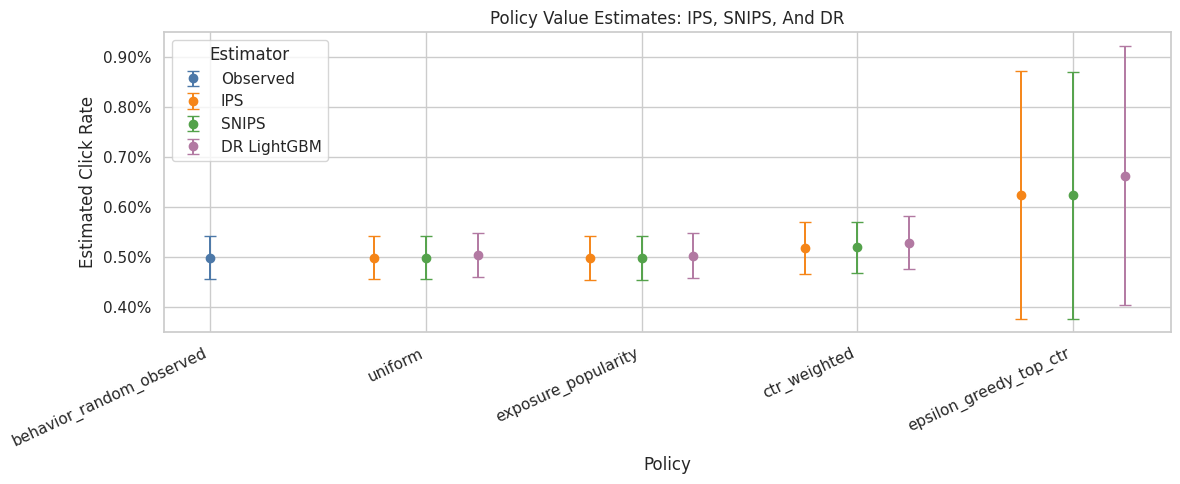
This output is part of the doubly robust off-policy evaluation workflow. Read it as a checkpoint that either verifies the log, defines reusable estimator machinery, or produces a diagnostic that motivates the next OPE step.
Direct Method Versus DR By Reward Model
This table compares direct method and DR estimates for both reward models.
The direct method is fully model-based. DR adds the residual correction. If the correction is large, it means observed outcomes disagree with the reward model in a way that matters for that policy. Large corrections are not automatically bad, but they deserve interpretation.
dm_dr_table = estimate_table[estimate_table["estimator"].isin(["DM", "DR"])].copy()
dm_dr_table = dm_dr_table[
    [
        "policy",
        "reward_model",
        "estimator",
        "estimate",
        "ci_95_lower",
        "ci_95_upper",
        "lift_pp",
        "relative_lift_pct",
        "mean_abs_correction",
        "mean_correction",
    ]
].sort_values(["policy", "reward_model", "estimator"])

dm_dr_table| policy | reward_model | estimator | estimate | ci_95_lower | ci_95_upper | lift_pp | relative_lift_pct | mean_abs_correction | mean_correction | |
|---|---|---|---|---|---|---|---|---|---|---|
| 17 | ctr_weighted | lightgbm | DM | 0.006021 | 0.005989 | 0.006052 | 0.104055 | 20.894635 | 0.011017 | -0.000741 |
| 18 | ctr_weighted | lightgbm | DR | 0.005280 | 0.004756 | 0.005803 | 0.029956 | 6.015257 | 0.011017 | -0.000741 |
| 15 | ctr_weighted | logistic | DM | 0.007355 | 0.007328 | 0.007382 | 0.237523 | 47.695402 | 0.012451 | -0.002195 |
| 16 | ctr_weighted | logistic | DR | 0.005160 | 0.004634 | 0.005687 | 0.018048 | 3.624090 | 0.012451 | -0.002195 |
| 23 | epsilon_greedy_top_ctr | lightgbm | DM | 0.011740 | 0.011607 | 0.011873 | 0.676002 | 135.743313 | 0.017472 | -0.005122 |
| 24 | epsilon_greedy_top_ctr | lightgbm | DR | 0.006618 | 0.004023 | 0.009214 | 0.163824 | 32.896440 | 0.017472 | -0.005122 |
| 21 | epsilon_greedy_top_ctr | logistic | DM | 0.014628 | 0.014580 | 0.014676 | 0.964777 | 193.730292 | 0.020619 | -0.008321 |
| 22 | epsilon_greedy_top_ctr | logistic | DR | 0.006306 | 0.003799 | 0.008814 | 0.132637 | 26.633840 | 0.020619 | -0.008321 |
| 11 | exposure_popularity | lightgbm | DM | 0.004913 | 0.004888 | 0.004938 | -0.006709 | -1.347183 | 0.009779 | 0.000108 |
| 12 | exposure_popularity | lightgbm | DR | 0.005021 | 0.004578 | 0.005463 | 0.004067 | 0.816622 | 0.009779 | 0.000108 |
| 9 | exposure_popularity | logistic | DM | 0.005733 | 0.005711 | 0.005754 | 0.075267 | 15.113877 | 0.010630 | -0.000756 |
| 10 | exposure_popularity | logistic | DR | 0.004977 | 0.004535 | 0.005418 | -0.000340 | -0.068183 | 0.010630 | -0.000756 |
| 5 | uniform | lightgbm | DM | 0.004943 | 0.004918 | 0.004968 | -0.003706 | -0.744091 | 0.009813 | 0.000092 |
| 6 | uniform | lightgbm | DR | 0.005035 | 0.004592 | 0.005477 | 0.005491 | 1.102546 | 0.009813 | 0.000092 |
| 3 | uniform | logistic | DM | 0.005786 | 0.005764 | 0.005807 | 0.080553 | 16.175230 | 0.010685 | -0.000794 |
| 4 | uniform | logistic | DR | 0.004992 | 0.004550 | 0.005434 | 0.001201 | 0.241083 | 0.010685 | -0.000794 |
Comparing DM and DR shows how much the residual correction changes the model-only estimate. Large differences mean observed logged rewards are correcting the reward model substantially.
Plot Direct Method Versus DR
This plot focuses only on model-based estimators. It shows how much the DR correction moves the direct-method estimates for each reward model.
The labels combine estimator and reward model, for example DR lightgbm. This avoids overloading Seaborn with multiple grouping variables and makes the comparison easier to read.
dm_dr_plot = dm_dr_table.copy()
dm_dr_plot["estimator_model"] = dm_dr_plot["estimator"] + " " + dm_dr_plot["reward_model"]

fig, ax = plt.subplots(figsize=(12, 5))
sns.pointplot(
    data=dm_dr_plot,
    x="policy",
    y="estimate",
    hue="estimator_model",
    dodge=0.45,
    errorbar=None,
    ax=ax,
)
ax.set_title("Direct Method Versus Doubly Robust Estimates")
ax.set_xlabel("Policy")
ax.set_ylabel("Estimated Click Rate")
ax.tick_params(axis="x", rotation=25)
ax.yaxis.set_major_formatter(lambda y, _: f"{y:.2%}")
ax.legend(title="Estimator / reward model", bbox_to_anchor=(1.02, 1), loc="upper left")
plt.tight_layout()
plt.show()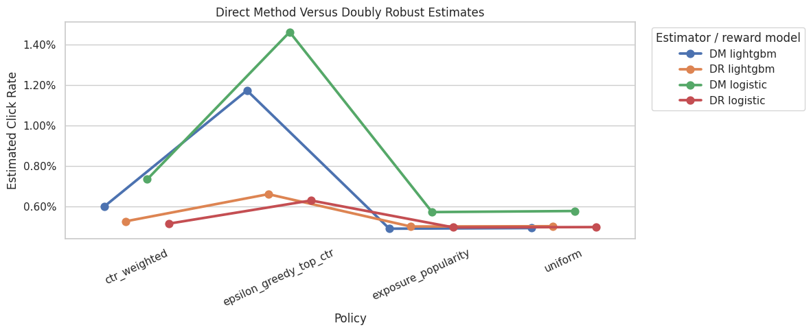
Comparing DM and DR shows how much the residual correction changes the model-only estimate. Large differences mean observed logged rewards are correcting the reward model substantially.
DR Correction Diagnostics
This cell summarizes the size of the residual correction in the DR estimator. The correction term is:
weight * (Y - q_hat(X, A))
A correction near zero on average means the direct method already aligns with observed residuals under that policy. A larger correction means the logged outcomes are materially changing the model-based estimate.
correction_diagnostics = (
    estimate_table.query("estimator == 'DR'")
    [["policy", "reward_model", "mean_correction", "mean_abs_correction", "ess_share", "max_weight"]]
    .sort_values("mean_abs_correction", ascending=False)
)

correction_diagnostics| policy | reward_model | mean_correction | mean_abs_correction | ess_share | max_weight | |
|---|---|---|---|---|---|---|
| 22 | epsilon_greedy_top_ctr | logistic | -0.008321 | 0.020619 | 0.040290 | 29.050000 |
| 24 | epsilon_greedy_top_ctr | lightgbm | -0.005122 | 0.017472 | 0.040290 | 29.050000 |
| 16 | ctr_weighted | logistic | -0.002195 | 0.012451 | 0.790628 | 2.740842 |
| 18 | ctr_weighted | lightgbm | -0.000741 | 0.011017 | 0.790628 | 2.740842 |
| 4 | uniform | logistic | -0.000794 | 0.010685 | 1.000000 | 1.000000 |
| 10 | exposure_popularity | logistic | -0.000756 | 0.010630 | 0.996399 | 1.132200 |
| 6 | uniform | lightgbm | 0.000092 | 0.009813 | 1.000000 | 1.000000 |
| 12 | exposure_popularity | lightgbm | 0.000108 | 0.009779 | 0.996399 | 1.132200 |
The correction diagnostics reveal how much of the DR estimate comes from importance-weighted residuals. Large or unstable corrections point to either support issues, reward-model misspecification, or both.
LightGBM Feature Importance
This cell extracts the top LightGBM feature importances after preprocessing.
Feature importance is not a causal explanation. It only tells us which transformed features the reward model used for prediction. Still, it is useful for debugging and storytelling: a sensible model should use item identity, position, user features, item metadata, or affinity signals rather than random artifacts.
lightgbm_pipeline = reward_models["lightgbm"]
feature_names = lightgbm_pipeline.named_steps["preprocess"].get_feature_names_out()
feature_importances = lightgbm_pipeline.named_steps["model"].feature_importances_

importance_df = (
    pd.DataFrame({"feature": feature_names, "importance": feature_importances})
    .sort_values("importance", ascending=False)
    .head(20)
)

fig, ax = plt.subplots(figsize=(9, 6))
sns.barplot(data=importance_df.sort_values("importance"), x="importance", y="feature", ax=ax, color="#4C78A8")
ax.set_title("Top LightGBM Reward Model Features")
ax.set_xlabel("Feature Importance")
ax.set_ylabel("Feature")
plt.tight_layout()
plt.show()

importance_df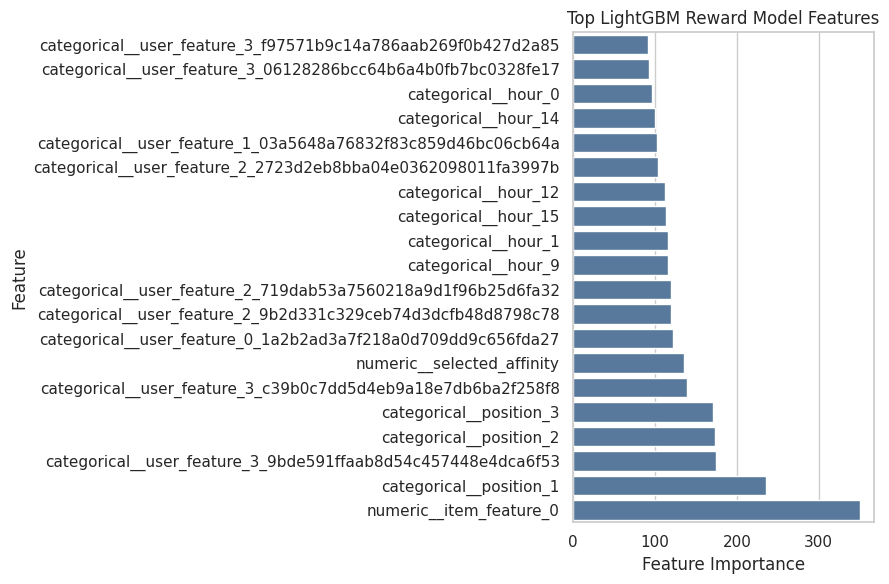
| feature | importance | |
|---|---|---|
| 119 | numeric__item_feature_0 | 350 |
| 0 | categorical__position_1 | 236 |
| 87 | categorical__user_feature_3_9bde591ffaab8d54c4... | 174 |
| 1 | categorical__position_2 | 173 |
| 2 | categorical__position_3 | 171 |
| 88 | categorical__user_feature_3_c39b0c7dd5d4eb9a18... | 139 |
| 118 | numeric__selected_affinity | 136 |
| 61 | categorical__user_feature_0_1a2b2ad3a7f218a0d7... | 122 |
| 77 | categorical__user_feature_2_9b2d331c329ceb74d3... | 120 |
| 74 | categorical__user_feature_2_719dab53a7560218a9... | 119 |
| 12 | categorical__hour_9 | 116 |
| 4 | categorical__hour_1 | 116 |
| 18 | categorical__hour_15 | 114 |
| 15 | categorical__hour_12 | 112 |
| 71 | categorical__user_feature_2_2723d2eb8bba04e036... | 104 |
| 65 | categorical__user_feature_1_03a5648a76832f83c8... | 103 |
| 17 | categorical__hour_14 | 100 |
| 3 | categorical__hour_0 | 96 |
| 82 | categorical__user_feature_3_06128286bcc64b6a4b... | 93 |
| 90 | categorical__user_feature_3_f97571b9c14a786aab... | 92 |
Feature importance helps explain what the reward model uses to predict clicks. These importances support model interpretation, but they should not be read as causal effects of the features themselves.
Weight And Model Diagnostics Together
This cell brings together the two main sources of uncertainty:
- importance-weight stability
- reward-model quality
A good DR estimate should have reasonable support and a reward model that is at least directionally predictive. Weak weights plus a weak reward model would make any offline policy conclusion fragile.
lightgbm_metric_row = reward_model_metrics.query("reward_model == 'lightgbm'").iloc[0]
combined_diagnostics = (
    estimate_table.query("estimator == 'DR' and reward_model == 'lightgbm'")
    [["policy", "estimate", "lift_pp", "ess_share", "mean_weight", "max_weight", "mean_abs_correction"]]
    .assign(
        reward_model_auc=lightgbm_metric_row["auc"],
        reward_model_log_loss=lightgbm_metric_row["log_loss"],
        reward_model_brier=lightgbm_metric_row["brier_score"],
    )
    .sort_values("estimate", ascending=False)
)

combined_diagnostics| policy | estimate | lift_pp | ess_share | mean_weight | max_weight | mean_abs_correction | reward_model_auc | reward_model_log_loss | reward_model_brier | |
|---|---|---|---|---|---|---|---|---|---|---|
| 24 | epsilon_greedy_top_ctr | 0.006618 | 0.163824 | 0.040290 | 1.001105 | 29.050000 | 0.017472 | 0.533007 | 0.034352 | 0.005104 |
| 18 | ctr_weighted | 0.005280 | 0.029956 | 0.790628 | 0.996987 | 2.740842 | 0.011017 | 0.533007 | 0.034352 | 0.005104 |
| 6 | uniform | 0.005035 | 0.005491 | 1.000000 | 1.000000 | 1.000000 | 0.009813 | 0.533007 | 0.034352 | 0.005104 |
| 12 | exposure_popularity | 0.005021 | 0.004067 | 0.996399 | 1.000591 | 1.132200 | 0.009779 | 0.533007 | 0.034352 | 0.005104 |
Combining weight and model diagnostics gives a fuller risk picture than policy value alone. A policy should look good not only on estimated reward, but also on support, ESS, and model quality.
Main Notebook Result Table
This final result table is the compact version to reference in a portfolio writeup.
It focuses on LightGBM DR because that is the strongest reward-model version in this notebook, while still retaining IPS and SNIPS as benchmarks from the previous notebook. The best policy should be interpreted alongside ESS, confidence intervals, and the observational limitations of logged bandit data.
main_result_table = estimate_table[
    (estimate_table["estimator"].isin(["Observed", "IPS", "SNIPS"]))
    | ((estimate_table["estimator"] == "DR") & (estimate_table["reward_model"] == "lightgbm"))
].copy()
main_result_table = main_result_table[
    [
        "policy",
        "estimator",
        "reward_model",
        "estimate",
        "ci_95_lower",
        "ci_95_upper",
        "lift_pp",
        "relative_lift_pct",
        "ess_share",
        "mean_weight",
        "max_weight",
    ]
].sort_values(["estimate", "ess_share"], ascending=[False, False])

main_result_table| policy | estimator | reward_model | estimate | ci_95_lower | ci_95_upper | lift_pp | relative_lift_pct | ess_share | mean_weight | max_weight | |
|---|---|---|---|---|---|---|---|---|---|---|---|
| 24 | epsilon_greedy_top_ctr | DR | lightgbm | 0.006618 | 0.004023 | 0.009214 | 0.163824 | 32.896440 | 0.040290 | 1.001105 | 29.050000 |
| 19 | epsilon_greedy_top_ctr | IPS | none | 0.006238 | 0.003756 | 0.008720 | 0.125800 | 25.261044 | 0.040290 | 1.001105 | 29.050000 |
| 20 | epsilon_greedy_top_ctr | SNIPS | none | 0.006231 | 0.003759 | 0.008703 | 0.125111 | 25.122784 | 0.040290 | 1.001105 | 29.050000 |
| 18 | ctr_weighted | DR | lightgbm | 0.005280 | 0.004756 | 0.005803 | 0.029956 | 6.015257 | 0.790628 | 0.996987 | 2.740842 |
| 14 | ctr_weighted | SNIPS | none | 0.005188 | 0.004675 | 0.005701 | 0.020806 | 4.178004 | 0.790628 | 0.996987 | 2.740842 |
| 13 | ctr_weighted | IPS | none | 0.005172 | 0.004660 | 0.005685 | 0.019244 | 3.864167 | 0.790628 | 0.996987 | 2.740842 |
| 6 | uniform | DR | lightgbm | 0.005035 | 0.004592 | 0.005477 | 0.005491 | 1.102546 | 1.000000 | 1.000000 | 1.000000 |
| 12 | exposure_popularity | DR | lightgbm | 0.005021 | 0.004578 | 0.005463 | 0.004067 | 0.816622 | 0.996399 | 1.000591 | 1.132200 |
| 1 | uniform | IPS | none | 0.004980 | 0.004544 | 0.005416 | 0.000000 | 0.000000 | 1.000000 | 1.000000 | 1.000000 |
| 0 | behavior_random_observed | Observed | none | 0.004980 | 0.004544 | 0.005416 | 0.000000 | 0.000000 | 1.000000 | 1.000000 | 1.000000 |
| 2 | uniform | SNIPS | none | 0.004980 | 0.004544 | 0.005416 | 0.000000 | 0.000000 | 1.000000 | 1.000000 | 1.000000 |
| 7 | exposure_popularity | IPS | none | 0.004971 | 0.004535 | 0.005407 | -0.000904 | -0.181598 | 0.996399 | 1.000591 | 1.132200 |
| 8 | exposure_popularity | SNIPS | none | 0.004968 | 0.004532 | 0.005404 | -0.001198 | -0.240522 | 0.996399 | 1.000591 | 1.132200 |
This output is part of the doubly robust off-policy evaluation workflow. Read it as a checkpoint that either verifies the log, defines reusable estimator machinery, or produces a diagnostic that motivates the next OPE step.
Notebook 4 Takeaways
This notebook introduced doubly robust OPE for the Open Bandit project.
The key ideas are:
- IPS and SNIPS use propensities and observed rewards directly.
- The direct method uses a reward model to predict outcomes for every candidate action.
- Doubly robust OPE combines the direct method with an IPS-style residual correction.
- Reward-model diagnostics matter because DR is only useful if the model contains real signal.
- Weight diagnostics still matter because the residual correction uses importance weights.
- Comparing logistic DR and LightGBM DR is a useful sensitivity check.
The next notebook should focus on policy comparison and sensitivity: clipping thresholds, alternate reward models, train/evaluation split sensitivity, and a polished recommendation about which policy is most credible offline.