06 - Sensitivity And Limitations

Goal: stress-test the causal conclusions before writing the final project memo.

The previous notebooks built a coherent causal story: raw rank-position patterns, IPW adjustment, doubly robust estimation, heterogeneous effects, and policy simulation. This notebook asks the uncomfortable but necessary question:

How robust are these results to modeling choices, overlap assumptions, treatment definitions, and unobserved risks?

This is the notebook that makes the project more credible. It shows that we understand the assumptions behind the estimates and do not overclaim from observational logged data.

What Can Go Wrong?

A causal estimate from logged recommendation data can fail for several reasons:

• Poor overlap: some rows are almost always top-ranked or almost always lower-ranked, leaving weak comparisons.
• Extreme IPW weights: a few rows can dominate weighted estimates.
• Feature-set dependence: results may change depending on which covariates are included.
• Treatment-definition dependence: top 1, top 3, and top 10 are different interventions.
• Unobserved confounding: missing ranker scores, user intent, or freshness signals may bias estimates.
• Metric limitation: clicks are short-term engagement, not necessarily long-term satisfaction.

The purpose of this notebook is not to eliminate every risk. The purpose is to measure obvious sensitivities, document limitations, and identify what would be needed for stronger evidence.

Notebook Setup

This cell imports the libraries used in the sensitivity analysis. We use pandas and numpy for data work, seaborn and matplotlib for plots, and scikit-learn for the nuisance models used in the doubly robust estimator.

from pathlib import Path

import matplotlib.pyplot as plt
import numpy as np
import pandas as pd
import seaborn as sns
from sklearn.base import clone
from sklearn.compose import ColumnTransformer
from sklearn.impute import SimpleImputer
from sklearn.linear_model import LogisticRegression
from sklearn.metrics import average_precision_score, brier_score_loss, roc_auc_score
from sklearn.model_selection import StratifiedKFold
from sklearn.pipeline import Pipeline
from sklearn.preprocessing import OneHotEncoder, StandardScaler

sns.set_theme(style="whitegrid")
pd.set_option("display.max_columns", 100)
pd.set_option("display.float_format", "{:.4f}".format)

This cell prepares the notebook environment for robustness, sensitivity checks, and limitations. There is no substantive model result yet; the important outcome is that the imports and display settings are ready so the next cells can focus on the data and causal question.

Load The Processed Dataset

This cell loads the processed impression-level MIND-small table. Each row is a displayed item inside an impression. The same processed file has been used throughout the project, so sensitivity results are directly comparable with earlier notebooks.

DATA_RELATIVE_PATH = Path("data/processed/mind_small_impressions_train_sample.parquet")
PROJECT_ROOT = next(
    path
    for path in [Path.cwd(), *Path.cwd().parents]
    if (path / DATA_RELATIVE_PATH).exists()
)

DATA_PATH = PROJECT_ROOT / DATA_RELATIVE_PATH
df = pd.read_parquet(DATA_PATH)

df.shape

(737762, 20)

The loaded table preview and shape confirm that the notebook is using the expected processed dataset. This check anchors the rest of the analysis, because all treatment, outcome, and covariate definitions depend on these columns being present and correctly typed.

Modeling Sample

Sensitivity analysis reruns models many times. To keep the notebook interactive, we use a fixed random sample smaller than the full processed table. The goal is not to produce the final number with maximum precision; it is to see whether the estimate is stable under reasonable changes.

Create Treatment Columns And Modeling Features

This cell creates a reusable modeling table. We keep the original is_top_3 treatment and also define is_top_10 for treatment-definition sensitivity. is_top_1 already exists in the processed table. log_item_exposures is a non-click popularity proxy used in the richer feature sets.

MODEL_SAMPLE_SIZE = 100_000
RANDOM_STATE = 42

model_df = (
    df.sample(n=min(len(df), MODEL_SAMPLE_SIZE), random_state=RANDOM_STATE)
    .reset_index(drop=True)
    .copy()
)

model_df["is_top_10"] = (model_df["rank_position"] <= 10).astype(int)
model_df["outcome"] = model_df["clicked"].astype(int)
model_df["log_item_exposures"] = np.log1p(model_df["item_exposures"])

pd.Series(
    {
        "rows": len(model_df),
        "click_rate": model_df["outcome"].mean(),
        "top_1_rate": model_df["is_top_1"].mean(),
        "top_3_rate": model_df["is_top_3"].mean(),
        "top_10_rate": model_df["is_top_10"].mean(),
    }
)

rows          100000.0000
click_rate         0.0396
top_1_rate         0.0269
top_3_rate         0.0802
top_10_rate        0.2359
dtype: float64

This cell defines the working analysis sample and standardizes treatment/outcome columns. Fixing this sample early keeps later model comparisons fair because each estimator works on the same rows and target definition.

Reusable Estimation Helpers

The sensitivity checks repeatedly estimate the same causal quantity under different settings. To avoid copying long model-fitting code several times, this section defines helper functions for preprocessing, AIPW estimation, IPW estimation, and confidence intervals.

Build Model Pipeline Helpers

This cell defines functions for creating sklearn pipelines. Numeric features are imputed and standardized. Categorical features are imputed and one-hot encoded. The code handles feature sets with or without categorical variables, which is useful for feature-set sensitivity.

def make_preprocessor(numeric_cols, categorical_cols):
    transformers = []
    if numeric_cols:
        numeric_pipeline = Pipeline(
            steps=[
                ("imputer", SimpleImputer(strategy="median")),
                ("scaler", StandardScaler()),
            ]
        )
        transformers.append(("num", numeric_pipeline, numeric_cols))

    if categorical_cols:
        categorical_pipeline = Pipeline(
            steps=[
                ("imputer", SimpleImputer(strategy="most_frequent")),
                (
                    "onehot",
                    OneHotEncoder(
                        handle_unknown="infrequent_if_exist",
                        min_frequency=50,
                        sparse_output=True,
                    ),
                ),
            ]
        )
        transformers.append(("cat", categorical_pipeline, categorical_cols))

    return ColumnTransformer(transformers=transformers)


def make_logistic_pipeline(numeric_cols, categorical_cols):
    return Pipeline(
        steps=[
            ("preprocess", make_preprocessor(numeric_cols, categorical_cols)),
            (
                "model",
                LogisticRegression(
                    max_iter=500,
                    solver="lbfgs",
                    n_jobs=-1,
                    random_state=RANDOM_STATE,
                ),
            ),
        ]
    )

This cell creates reusable modeling machinery rather than a final result. The value is consistency: the same preprocessing and helper functions can be applied across folds, estimators, and sensitivity checks.

Define AIPW And IPW Estimation Helpers

This cell defines the main estimation functions. estimate_aipw cross-fits propensity and outcome models, computes per-row AIPW scores, and returns both the scored data and a summary table. estimate_ipw_lift estimates the IPW-adjusted lift from already-computed propensity scores and allows optional weight capping.

def weighted_mean(values, weights):
    values = np.asarray(values, dtype=float)
    weights = np.asarray(weights, dtype=float)
    return np.sum(values * weights) / np.sum(weights)


def effective_sample_size(weights):
    weights = np.asarray(weights, dtype=float)
    return weights.sum() ** 2 / np.sum(weights**2)


def estimate_ipw_lift(scored_df, eps=0.01, cap_quantile=None):
    e = scored_df["e_hat"].clip(eps, 1 - eps).to_numpy()
    treatment = scored_df["treatment"].to_numpy()
    outcome = scored_df["outcome"].to_numpy()
    weights = np.where(treatment == 1, 1 / e, 1 / (1 - e))

    if cap_quantile is not None:
        weights = np.clip(weights, None, np.quantile(weights, cap_quantile))

    treated = treatment == 1
    control = ~treated
    treated_mean = weighted_mean(outcome[treated], weights[treated])
    control_mean = weighted_mean(outcome[control], weights[control])

    return {
        "ipw_treated_ctr": treated_mean,
        "ipw_control_ctr": control_mean,
        "ipw_lift": treated_mean - control_mean,
        "max_weight": weights.max(),
        "effective_sample_size": effective_sample_size(weights),
    }


def estimate_aipw(data, treatment_col, numeric_features, categorical_features, n_folds=2, eps=0.01):
    work = data.copy().reset_index(drop=True)
    work["treatment"] = work[treatment_col].astype(int)
    work["outcome"] = work["clicked"].astype(int)

    propensity_features = numeric_features + categorical_features
    outcome_numeric_features = numeric_features + ["treatment"]
    outcome_features = outcome_numeric_features + categorical_features

    base_propensity_model = make_logistic_pipeline(numeric_features, categorical_features)
    base_outcome_model = make_logistic_pipeline(outcome_numeric_features, categorical_features)

    e_hat = np.zeros(len(work))
    mu1_hat = np.zeros(len(work))
    mu0_hat = np.zeros(len(work))
    propensity_metrics = []
    outcome_metrics = []

    splitter = StratifiedKFold(n_splits=n_folds, shuffle=True, random_state=RANDOM_STATE)

    for fold, (train_idx, valid_idx) in enumerate(splitter.split(work[propensity_features], work["treatment"]), start=1):
        train_df = work.iloc[train_idx]
        valid_df = work.iloc[valid_idx]

        propensity_model = clone(base_propensity_model)
        propensity_model.fit(train_df[propensity_features], train_df["treatment"])
        e_valid = propensity_model.predict_proba(valid_df[propensity_features])[:, 1]
        e_hat[valid_idx] = e_valid

        outcome_model = clone(base_outcome_model)
        outcome_model.fit(train_df[outcome_features], train_df["outcome"])

        valid_actual = valid_df[outcome_features]
        y_valid_hat = outcome_model.predict_proba(valid_actual)[:, 1]

        valid_treated = valid_df[propensity_features].copy()
        valid_treated["treatment"] = 1
        valid_treated = valid_treated[outcome_features]

        valid_control = valid_df[propensity_features].copy()
        valid_control["treatment"] = 0
        valid_control = valid_control[outcome_features]

        mu1_hat[valid_idx] = outcome_model.predict_proba(valid_treated)[:, 1]
        mu0_hat[valid_idx] = outcome_model.predict_proba(valid_control)[:, 1]

        propensity_metrics.append(
            {
                "fold": fold,
                "roc_auc": roc_auc_score(valid_df["treatment"], e_valid),
                "average_precision": average_precision_score(valid_df["treatment"], e_valid),
                "brier_score": brier_score_loss(valid_df["treatment"], e_valid),
            }
        )
        outcome_metrics.append(
            {
                "fold": fold,
                "roc_auc": roc_auc_score(valid_df["outcome"], y_valid_hat),
                "average_precision": average_precision_score(valid_df["outcome"], y_valid_hat),
                "brier_score": brier_score_loss(valid_df["outcome"], y_valid_hat),
            }
        )

    work["e_hat"] = e_hat
    work["mu1_hat"] = mu1_hat
    work["mu0_hat"] = mu0_hat
    work["mu_diff_hat"] = work["mu1_hat"] - work["mu0_hat"]

    e = work["e_hat"].clip(eps, 1 - eps).to_numpy()
    treatment = work["treatment"].to_numpy()
    outcome = work["outcome"].to_numpy()
    mu1 = work["mu1_hat"].to_numpy()
    mu0 = work["mu0_hat"].to_numpy()

    work["aipw_score"] = (mu1 - mu0) + treatment * (outcome - mu1) / e - (1 - treatment) * (outcome - mu0) / (1 - e)

    naive_treated = work.loc[work["treatment"] == 1, "outcome"].mean()
    naive_control = work.loc[work["treatment"] == 0, "outcome"].mean()
    dr_ate = work["aipw_score"].mean()
    dr_se = work["aipw_score"].std(ddof=1) / np.sqrt(len(work))
    ipw = estimate_ipw_lift(work, eps=eps, cap_quantile=0.99)

    summary = {
        "treatment_col": treatment_col,
        "rows": len(work),
        "treatment_rate": work["treatment"].mean(),
        "naive_lift": naive_treated - naive_control,
        "ipw_lift_99cap": ipw["ipw_lift"],
        "outcome_regression_lift": work["mu_diff_hat"].mean(),
        "dr_lift": dr_ate,
        "standard_error": dr_se,
        "ci_95_lower": dr_ate - 1.96 * dr_se,
        "ci_95_upper": dr_ate + 1.96 * dr_se,
        "propensity_auc_mean": pd.DataFrame(propensity_metrics)["roc_auc"].mean(),
        "outcome_auc_mean": pd.DataFrame(outcome_metrics)["roc_auc"].mean(),
    }

    return work, summary, pd.DataFrame(propensity_metrics), pd.DataFrame(outcome_metrics)

This cell creates reusable modeling machinery rather than a final result. The value is consistency: the same preprocessing and helper functions can be applied across folds, estimators, and sensitivity checks.

Baseline Estimate

Before running sensitivity checks, we create one baseline estimate for the main treatment: is_top_3. This uses the richer feature set from earlier notebooks and 2-fold cross-fitting to keep repeated sensitivity runs manageable.

Define The Baseline Feature Set

This cell defines the baseline covariates. The feature set includes user history, slate size, text-length proxies, time context, item exposure, category, and subcategory. This is the main adjustment set used in later sensitivity comparisons.

full_numeric_features = [
    "history_len",
    "candidate_set_size",
    "title_length",
    "abstract_length",
    "hour",
    "day_of_week",
    "log_item_exposures",
]
full_categorical_features = ["category", "subcategory"]

full_numeric_features, full_categorical_features

(['history_len',
  'candidate_set_size',
  'title_length',
  'abstract_length',
  'hour',
  'day_of_week',
  'log_item_exposures'],
 ['category', 'subcategory'])

The feature-set sensitivity checks whether the estimated lift depends heavily on one adjustment specification. Robustness across feature sets gives more confidence than a result that only appears under one model.

Estimate The Baseline Top-3 Effect

This cell runs the baseline doubly robust estimator. It returns the scored dataset with nuisance predictions and AIPW scores, plus a summary table with naive, IPW, outcome-regression, and doubly robust estimates.

baseline_scored, baseline_summary, baseline_propensity_metrics, baseline_outcome_metrics = estimate_aipw(
    model_df,
    treatment_col="is_top_3",
    numeric_features=full_numeric_features,
    categorical_features=full_categorical_features,
    n_folds=2,
    eps=0.01,
)

pd.DataFrame([baseline_summary])

	treatment_col	rows	treatment_rate	naive_lift	ipw_lift_99cap	outcome_regression_lift	dr_lift	standard_error	ci_95_lower	ci_95_upper	propensity_auc_mean	outcome_auc_mean
0	is_top_3	100000	0.0802	0.0660	0.0180	0.0276	0.0121	0.0034	0.0054	0.0188	0.7701	0.6992

The baseline estimate is the reference point for all sensitivity checks. Later cells vary overlap, weights, features, and treatment definitions to see whether this estimate is robust.

Inspect Baseline Nuisance Model Metrics

This cell shows cross-fitted model metrics for the baseline propensity and outcome models. These metrics are diagnostics: they tell us whether the nuisance models have signal, but the causal estimate still depends on causal assumptions.

display(baseline_propensity_metrics)
display(baseline_outcome_metrics)

	fold	roc_auc	average_precision	brier_score
0	1	0.7719	0.3259	0.0664
1	2	0.7683	0.3271	0.0664

	fold	roc_auc	average_precision	brier_score
0	1	0.6994	0.1081	0.0365
1	2	0.6990	0.1151	0.0372

The nuisance-model metrics show how well the supporting prediction models perform. They are not the causal answer, but weak nuisance models can make IPW, DR, and policy estimates less reliable.

Overlap Sensitivity

Overlap means that comparable rows have some chance of being treated and some chance of being control. If estimated propensities are too close to 0 or 1, causal estimates rely on weak comparisons.

This section trims rows outside increasingly strict propensity ranges and recomputes the doubly robust estimate on the remaining population. The estimand changes as we trim: stricter thresholds estimate the effect for better-overlap rows only.

Recompute DR Lift Under Overlap Trimming

This cell filters rows to several propensity ranges such as [0.05, 0.95] and [0.10, 0.90]. For each range, it reports how many rows remain, the treatment rate among retained rows, and the DR lift using the retained AIPW scores.

overlap_rows = []
for lower, upper in [(0.01, 0.99), (0.05, 0.95), (0.10, 0.90), (0.15, 0.85)]:
    kept = baseline_scored.query("@lower <= e_hat <= @upper")
    scores = kept["aipw_score"]
    se = scores.std(ddof=1) / np.sqrt(len(scores))
    overlap_rows.append(
        {
            "propensity_range": f"[{lower:.2f}, {upper:.2f}]",
            "rows_kept": len(kept),
            "share_kept": len(kept) / len(baseline_scored),
            "treatment_rate_kept": kept["treatment"].mean(),
            "dr_lift": scores.mean(),
            "standard_error": se,
            "ci_95_lower": scores.mean() - 1.96 * se,
            "ci_95_upper": scores.mean() + 1.96 * se,
        }
    )

overlap_sensitivity = pd.DataFrame(overlap_rows)
overlap_sensitivity

	propensity_range	rows_kept	share_kept	treatment_rate_kept	dr_lift	standard_error	ci_95_lower	ci_95_upper
0	[0.01, 0.99]	85484	0.8548	0.0907	0.0125	0.0028	0.0070	0.0181
1	[0.05, 0.95]	53286	0.5329	0.1264	0.0269	0.0029	0.0212	0.0325
2	[0.10, 0.90]	32670	0.3267	0.1709	0.0391	0.0039	0.0316	0.0467
3	[0.15, 0.85]	18368	0.1837	0.2324	0.0575	0.0057	0.0463	0.0687

The overlap sensitivity results show how the estimate changes when low-overlap rows are removed. Stability here supports the claim that the effect is not driven only by hard-to-compare observations.

Plot Overlap Sensitivity

This cell plots the DR lift under each trimming rule. If estimates are stable as overlap becomes stricter, that supports robustness. If estimates change sharply, the result may be driven by low-overlap observations.

plt.figure(figsize=(9, 5))
sns.pointplot(data=overlap_sensitivity, x="propensity_range", y="dr_lift")
plt.axhline(0, color="black", linewidth=1)
plt.title("DR Lift Under Propensity Overlap Trimming")
plt.xlabel("Retained propensity range")
plt.ylabel("Doubly robust lift")
plt.tight_layout()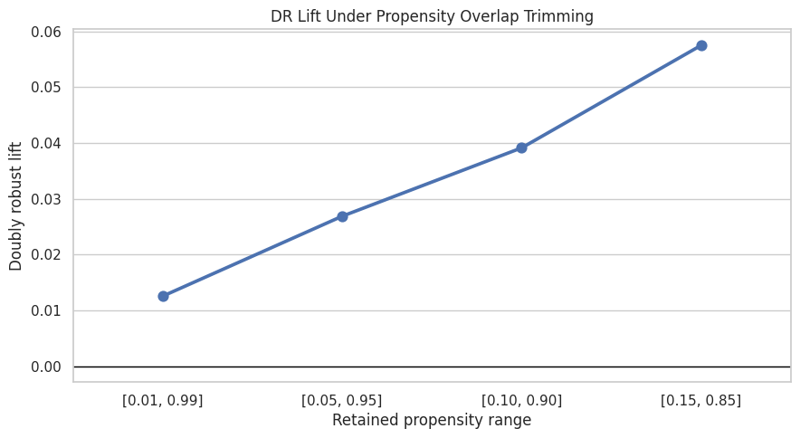

The overlap sensitivity results show how the estimate changes when low-overlap rows are removed. Stability here supports the claim that the effect is not driven only by hard-to-compare observations.

Weight Sensitivity

IPW estimates can be unstable when some rows receive very large weights. Earlier notebooks used capped weights. Here we compare several cap choices to see whether IPW lift depends heavily on extreme weights.

Compare IPW Weight Caps

This cell recomputes IPW lift with no weight cap and with caps at the 99.5th, 99th, and 95th percentiles. It also reports effective sample size. If tighter caps move the estimate dramatically, IPW is fragile.

weight_rows = []
for label, cap in [("no_cap", None), ("cap_99_5", 0.995), ("cap_99", 0.99), ("cap_95", 0.95)]:
    result = estimate_ipw_lift(baseline_scored, eps=0.01, cap_quantile=cap)
    weight_rows.append({"weight_rule": label, **result})

weight_sensitivity = pd.DataFrame(weight_rows)
weight_sensitivity

	weight_rule	ipw_treated_ctr	ipw_control_ctr	ipw_lift	max_weight	effective_sample_size
0	no_cap	0.0429	0.0360	0.0069	100.0000	8549.2487
1	cap_99_5	0.0463	0.0360	0.0103	56.4496	13201.5961
2	cap_99	0.0540	0.0360	0.0180	26.7517	23108.0017
3	cap_95	0.0875	0.0360	0.0515	5.0305	66230.5762

The weight calculation translates propensity scores into reweighting factors for the observed data. Stabilization and clipping protect the estimate from a few extreme-propensity rows dominating the result.

Plot Weight Sensitivity

This cell plots IPW lift under different weight caps. Stable estimates across cap choices are reassuring. Large swings suggest the weighted estimate depends on a small number of high-weight observations.

plt.figure(figsize=(8, 5))
sns.barplot(data=weight_sensitivity, x="weight_rule", y="ipw_lift")
plt.axhline(0, color="black", linewidth=1)
plt.title("IPW Lift Sensitivity To Weight Capping")
plt.xlabel("Weight rule")
plt.ylabel("IPW lift")
plt.tight_layout()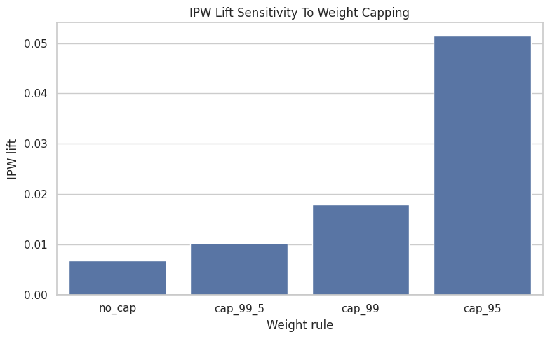

The weight-cap sensitivity checks whether extreme inverse-probability weights control the estimate. If the estimate is stable across caps, the result is less dependent on a few influential rows.

Feature-Set Sensitivity

Causal adjustment depends on which observed covariates enter the nuisance models. If the estimate changes dramatically when we add reasonable features, the conclusion is model-dependent. If it remains directionally similar, the result is more credible.

Estimate Top-3 Lift Under Multiple Feature Sets

This cell compares three adjustment sets: simple context features, content/category features, and the fuller baseline feature set. The full feature-set result reuses the baseline estimate so we do not refit it unnecessarily.

feature_configs = {
    "simple_context": {
        "numeric": ["history_len", "candidate_set_size", "hour", "day_of_week"],
        "categorical": [],
    },
    "content_category": {
        "numeric": ["history_len", "candidate_set_size", "title_length", "abstract_length", "hour", "day_of_week"],
        "categorical": ["category"],
    },
    "full_context_content_exposure": {
        "numeric": full_numeric_features,
        "categorical": full_categorical_features,
    },
}

feature_sensitivity_rows = []
for feature_set, config in feature_configs.items():
    if feature_set == "full_context_content_exposure":
        summary = baseline_summary.copy()
    else:
        _, summary, _, _ = estimate_aipw(
            model_df,
            treatment_col="is_top_3",
            numeric_features=config["numeric"],
            categorical_features=config["categorical"],
            n_folds=2,
            eps=0.01,
        )
    summary["feature_set"] = feature_set
    feature_sensitivity_rows.append(summary)

feature_sensitivity = pd.DataFrame(feature_sensitivity_rows)
feature_sensitivity[
    [
        "feature_set",
        "naive_lift",
        "ipw_lift_99cap",
        "outcome_regression_lift",
        "dr_lift",
        "ci_95_lower",
        "ci_95_upper",
        "propensity_auc_mean",
        "outcome_auc_mean",
    ]
]

	feature_set	naive_lift	ipw_lift_99cap	outcome_regression_lift	dr_lift	ci_95_lower	ci_95_upper	propensity_auc_mean	outcome_auc_mean
0	simple_context	0.0660	0.0198	0.0299	0.0120	0.0057	0.0184	0.7768	0.6938
1	content_category	0.0660	0.0190	0.0289	0.0121	0.0056	0.0185	0.7750	0.6955
2	full_context_content_exposure	0.0660	0.0180	0.0276	0.0121	0.0054	0.0188	0.7701	0.6992

The feature-set sensitivity checks whether the estimated lift depends heavily on one adjustment specification. Robustness across feature sets gives more confidence than a result that only appears under one model.

Plot Feature-Set Sensitivity

This cell plots the doubly robust estimate across feature sets. Similar values suggest the result is not purely an artifact of one adjustment set. Meaningful differences tell us which covariates materially affect the causal estimate.

plt.figure(figsize=(10, 5))
sns.barplot(data=feature_sensitivity, x="feature_set", y="dr_lift")
plt.axhline(0, color="black", linewidth=1)
plt.title("DR Lift Sensitivity To Feature Set")
plt.xlabel("Feature set")
plt.ylabel("Doubly robust lift")
plt.xticks(rotation=20, ha="right")
plt.tight_layout()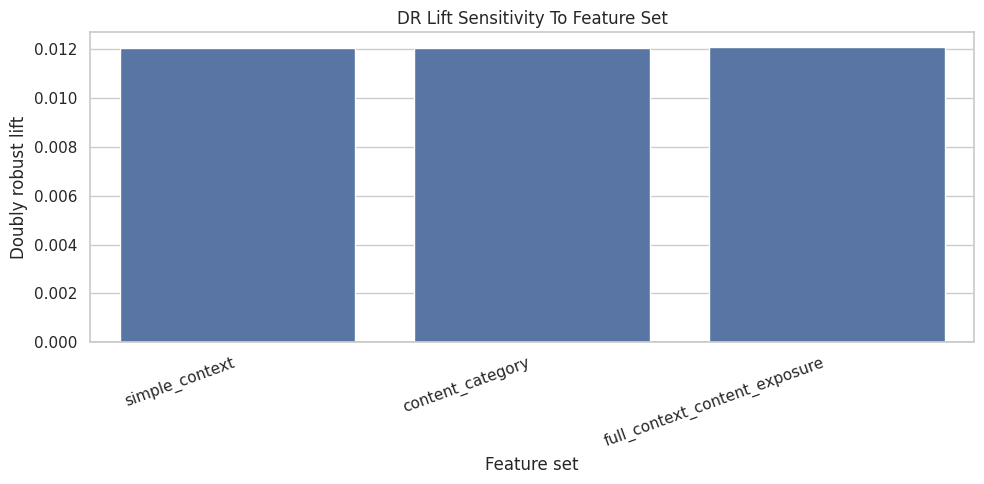

This output is part of the robustness, sensitivity checks, and limitations workflow. Read it as a checkpoint: it either verifies an input, defines reusable analysis machinery, or produces a diagnostic that motivates the next step in the notebook.

Treatment-Definition Sensitivity

The phrase “ranking position effect” can mean different interventions. Moving an item to rank 1 is not the same as moving it into the top 3 or top 10. This section compares related treatment definitions.

Estimate Effects For Top-1, Top-3, And Top-10 Exposure

This cell reruns the doubly robust estimator for three treatment definitions. These estimates are not interchangeable because each treatment has a different control group and different product meaning. The comparison shows whether the rank effect is concentrated at the very top or persists through broader high-visibility positions.

treatment_labels = {
    "is_top_1": "rank 1 vs lower",
    "is_top_3": "rank 1-3 vs lower",
    "is_top_10": "rank 1-10 vs lower",
}

treatment_sensitivity_rows = []
for treatment_col, treatment_label in treatment_labels.items():
    if treatment_col == "is_top_3":
        summary = baseline_summary.copy()
    else:
        _, summary, _, _ = estimate_aipw(
            model_df,
            treatment_col=treatment_col,
            numeric_features=full_numeric_features,
            categorical_features=full_categorical_features,
            n_folds=2,
            eps=0.01,
        )
    summary["treatment_definition"] = treatment_label
    treatment_sensitivity_rows.append(summary)

treatment_sensitivity = pd.DataFrame(treatment_sensitivity_rows)
treatment_sensitivity[
    [
        "treatment_definition",
        "treatment_rate",
        "naive_lift",
        "ipw_lift_99cap",
        "outcome_regression_lift",
        "dr_lift",
        "ci_95_lower",
        "ci_95_upper",
    ]
]

	treatment_definition	treatment_rate	naive_lift	ipw_lift_99cap	outcome_regression_lift	dr_lift	ci_95_lower	ci_95_upper
0	rank 1 vs lower	0.0269	0.0757	0.0390	0.0304	0.0120	0.0049	0.0191
1	rank 1-3 vs lower	0.0802	0.0660	0.0180	0.0276	0.0121	0.0054	0.0188
2	rank 1-10 vs lower	0.2359	0.0419	0.0097	0.0137	0.0111	0.0060	0.0162

The treatment-definition sensitivity asks whether the story changes when exposure is defined more narrowly or broadly. This helps clarify whether the finding is about top rank specifically or general high-rank visibility.

Plot Treatment-Definition Sensitivity

This cell plots the DR lift for the three treatment definitions. A larger top-1 effect than top-10 effect would suggest visibility is most valuable at the very top. A similar effect across definitions would suggest broader high-rank exposure matters.

plt.figure(figsize=(9, 5))
sns.barplot(data=treatment_sensitivity, x="treatment_definition", y="dr_lift")
plt.axhline(0, color="black", linewidth=1)
plt.title("DR Lift Sensitivity To Treatment Definition")
plt.xlabel("Treatment definition")
plt.ylabel("Doubly robust lift")
plt.xticks(rotation=15, ha="right")
plt.tight_layout()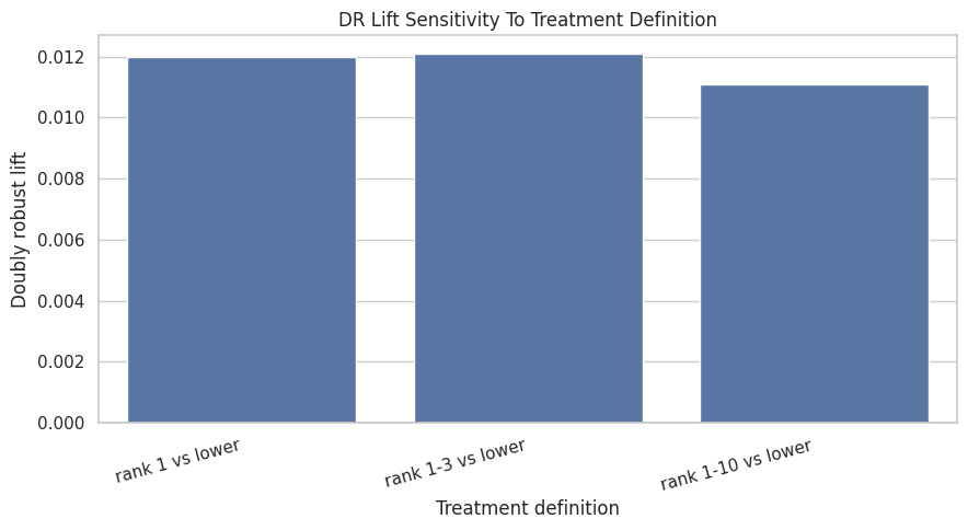

The treatment-definition sensitivity asks whether the story changes when exposure is defined more narrowly or broadly. This helps clarify whether the finding is about top rank specifically or general high-rank visibility.

Pre-Adjustment Imbalance Check

This is not a placebo test, but it is a useful control-style diagnostic. If treatment is strongly associated with pre-treatment covariates, then naive comparisons are clearly not credible. This check reinforces why causal adjustment was necessary.

Compute Standardized Mean Differences Before Adjustment

This cell computes standardized mean differences for numeric covariates comparing top-3 rows with lower-ranked rows before weighting. Large absolute values show imbalance between treatment and control groups.

def standardized_mean_difference(data, feature, treatment_col="is_top_3"):
    treated = data[treatment_col] == 1
    control = ~treated
    mean_t = data.loc[treated, feature].mean()
    mean_c = data.loc[control, feature].mean()
    var_t = data.loc[treated, feature].var(ddof=0)
    var_c = data.loc[control, feature].var(ddof=0)
    pooled_sd = np.sqrt((var_t + var_c) / 2)
    return (mean_t - mean_c) / pooled_sd if pooled_sd > 0 else np.nan


imbalance = pd.DataFrame(
    {
        "feature": full_numeric_features,
        "smd_before_adjustment": [standardized_mean_difference(model_df, feature) for feature in full_numeric_features],
    }
)
imbalance["abs_smd"] = imbalance["smd_before_adjustment"].abs()
imbalance.sort_values("abs_smd", ascending=False)

	feature	smd_before_adjustment	abs_smd
1	candidate_set_size	-0.9319	0.9319
6	log_item_exposures	0.3435	0.3435
0	history_len	-0.0641	0.0641
5	day_of_week	-0.0385	0.0385
2	title_length	0.0335	0.0335
4	hour	0.0130	0.0130
3	abstract_length	-0.0127	0.0127

The imbalance output documents the confounding problem before adjustment. This is useful in the limitations story because it shows why causal methods are needed and where unobserved confounding may still remain.

Plot Pre-Adjustment Imbalance

This cell visualizes covariate imbalance before adjustment. The dashed line at 0.1 is a common rough threshold. Features above that threshold differ meaningfully between top-3 and lower-ranked rows.

plt.figure(figsize=(9, 5))
sns.barplot(data=imbalance.sort_values("abs_smd", ascending=True), x="abs_smd", y="feature")
plt.axvline(0.1, color="black", linestyle="--", linewidth=1)
plt.title("Pre-Adjustment Numeric Covariate Imbalance")
plt.xlabel("Absolute standardized mean difference")
plt.ylabel("Feature")
plt.tight_layout()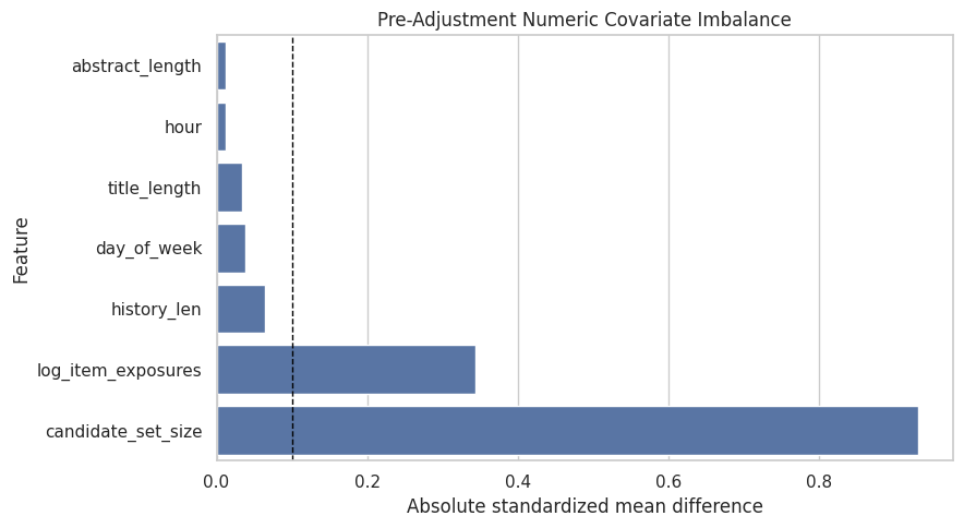

The imbalance output documents the confounding problem before adjustment. This is useful in the limitations story because it shows why causal methods are needed and where unobserved confounding may still remain.

Robustness Summary

This section gathers the main sensitivity results into compact tables. The goal is to make the final memo easier to write: which checks were reassuring, and which checks exposed fragility?

Combine Key Sensitivity Results

This cell creates a compact summary of baseline, feature-set, and treatment-definition sensitivity. It does not replace the detailed tables above, but it gives one place to compare the main estimates.

robustness_summary = pd.concat(
    [
        pd.DataFrame([baseline_summary]).assign(check="baseline", variant="top_3_full_features"),
        feature_sensitivity.rename(columns={"feature_set": "variant"}).assign(check="feature_set"),
        treatment_sensitivity.rename(columns={"treatment_definition": "variant"}).assign(check="treatment_definition"),
    ],
    ignore_index=True,
)

robustness_summary[["check", "variant", "treatment_rate", "naive_lift", "ipw_lift_99cap", "dr_lift", "ci_95_lower", "ci_95_upper"]]

	check	variant	treatment_rate	naive_lift	ipw_lift_99cap	dr_lift	ci_95_lower	ci_95_upper
0	baseline	top_3_full_features	0.0802	0.0660	0.0180	0.0121	0.0054	0.0188
1	feature_set	simple_context	0.0802	0.0660	0.0198	0.0120	0.0057	0.0184
2	feature_set	content_category	0.0802	0.0660	0.0190	0.0121	0.0056	0.0185
3	feature_set	full_context_content_exposure	0.0802	0.0660	0.0180	0.0121	0.0054	0.0188
4	treatment_definition	rank 1 vs lower	0.0269	0.0757	0.0390	0.0120	0.0049	0.0191
5	treatment_definition	rank 1-3 vs lower	0.0802	0.0660	0.0180	0.0121	0.0054	0.0188
6	treatment_definition	rank 1-10 vs lower	0.2359	0.0419	0.0097	0.0111	0.0060	0.0162

The robustness summary gathers the main sensitivity checks into one table. This makes it easier to state which conclusions are stable and which require caution.

Limitations Table

A strong causal portfolio project should state limitations directly. This table translates technical risks into product implications and next steps.

Create A Final Limitations Table

This cell creates a memo-ready limitations table. Each row describes a risk, why it matters, what this project did to reduce it, and what would improve the evidence in a real product setting.

limitations = pd.DataFrame(
    [
        {
            "risk": "Unobserved confounding",
            "why_it_matters": "The logged ranker may use relevance scores, freshness signals, or user intent features that are missing from this public dataset.",
            "what_we_did": "Adjusted for observed user history, slate size, content metadata, time, and item exposure proxies.",
            "what_would_improve_it": "Use production ranker scores, richer user/item features, or randomized ranking experiments.",
        },
        {
            "risk": "Limited overlap",
            "why_it_matters": "Some items may be almost deterministically top-ranked or lower-ranked, making counterfactual comparisons weak.",
            "what_we_did": "Inspected propensity overlap and recomputed estimates under trimming thresholds.",
            "what_would_improve_it": "Restrict claims to common-support regions or collect randomized exploration traffic.",
        },
        {
            "risk": "Extreme weights",
            "why_it_matters": "A few high-weight observations can dominate IPW estimates.",
            "what_we_did": "Compared IPW estimates under several weight caps and reported effective sample size.",
            "what_would_improve_it": "Use stabilized weights, overlap weighting, or stronger propensity models with calibration checks.",
        },
        {
            "risk": "Treatment definition ambiguity",
            "why_it_matters": "Top-1, top-3, and top-10 exposure correspond to different product interventions.",
            "what_we_did": "Estimated effects under multiple treatment definitions.",
            "what_would_improve_it": "Tie the treatment definition to a concrete UI or ranking-policy change.",
        },
        {
            "risk": "Clicks are short-term",
            "why_it_matters": "A click may not indicate satisfaction, watch time, retention, or long-term member value.",
            "what_we_did": "Used clicks because they are the available MIND outcome.",
            "what_would_improve_it": "Use downstream satisfaction, dwell time, retention, or long-term engagement metrics.",
        },
        {
            "risk": "Interference across items",
            "why_it_matters": "Promoting one item changes exposure for other items in the same slate.",
            "what_we_did": "Framed policy simulation as prioritization rather than a full re-ranking counterfactual.",
            "what_would_improve_it": "Evaluate full-slate policies with online experiments or slate-aware causal methods.",
        },
    ]
)

limitations

	risk	why_it_matters	what_we_did	what_would_improve_it
0	Unobserved confounding	The logged ranker may use relevance scores, fr...	Adjusted for observed user history, slate size...	Use production ranker scores, richer user/item...
1	Limited overlap	Some items may be almost deterministically top...	Inspected propensity overlap and recomputed es...	Restrict claims to common-support regions or c...
2	Extreme weights	A few high-weight observations can dominate IP...	Compared IPW estimates under several weight ca...	Use stabilized weights, overlap weighting, or ...
3	Treatment definition ambiguity	Top-1, top-3, and top-10 exposure correspond t...	Estimated effects under multiple treatment def...	Tie the treatment definition to a concrete UI ...
4	Clicks are short-term	A click may not indicate satisfaction, watch t...	Used clicks because they are the available MIN...	Use downstream satisfaction, dwell time, reten...
5	Interference across items	Promoting one item changes exposure for other ...	Framed policy simulation as prioritization rat...	Evaluate full-slate policies with online exper...

This cell creates reusable project artifacts for the writeup. Saving figures, tables, limitations, and resume bullets makes the analysis easier to present outside the notebook itself.

Final Interpretation Guidance

Use careful wording in the final project report. A good conclusion should say what the estimates suggest while naming the assumptions.

A strong version:

Across multiple adjustment strategies, top-ranked exposure is associated with a positive adjusted lift in click probability. The estimate is directionally robust across several sensitivity checks, but it remains an observational estimate that depends on measured confounding, overlap, and the click outcome. The results identify promising ranking-policy hypotheses for online experimentation rather than proving a production policy.

Avoid claiming:

Putting any item in the top 3 will always increase clicks by exactly X.

The portfolio win is not overconfidence. The win is showing that you can estimate, diagnose, stress-test, and communicate causal evidence like a product data scientist.