from pathlib import Path

import matplotlib.pyplot as plt
import numpy as np
import pandas as pd
import seaborn as sns
from sklearn.base import clone
from sklearn.compose import ColumnTransformer
from sklearn.impute import SimpleImputer
from sklearn.linear_model import LogisticRegression
from sklearn.metrics import average_precision_score, brier_score_loss, roc_auc_score
from sklearn.model_selection import StratifiedKFold
from sklearn.pipeline import Pipeline
from sklearn.preprocessing import OneHotEncoder, StandardScaler

sns.set_theme(style="whitegrid")
pd.set_option("display.max_columns", 100)
pd.set_option("display.float_format", "{:.4f}".format)04 - Heterogeneous Treatment Effects
Goal: estimate where top-3 ranking exposure appears to matter more or less.
The previous notebooks estimated an average effect of is_top_3 on clicked. That global estimate is useful, but product teams usually need a more targeted answer:
For which users, items, and contexts does higher ranking position create the most incremental engagement?
This notebook uses doubly robust/AIPW scores to estimate segment-level effects across content categories, user-history buckets, candidate-set-size buckets, item-exposure buckets, and time-of-day buckets.
Why Heterogeneous Effects Matter
A single average treatment effect can hide important product differences. For example, top-3 placement might be very valuable for fresh entertainment content, but less valuable for items that users would click regardless of position. It might also matter more when users face long recommendation lists because lower positions become harder to notice.
For a recommendation data science portfolio project, this notebook is important because it turns the causal estimate into a product decision framework:
- Which segments are most position-sensitive?
- Which segments have little incremental benefit from top placement?
- Where might ranking changes produce the biggest engagement return?
- Where do we need more data or better overlap before making claims?
Notebook Setup
This cell imports the libraries used for heterogeneous effect estimation. Most of the workflow is standard pandas/numpy analysis plus scikit-learn nuisance models. We reuse the doubly robust logic from notebook 3 so notebook 4 can run independently.
This cell prepares the notebook environment for heterogeneous treatment effects across product segments. There is no substantive model result yet; the important outcome is that the imports and display settings are ready so the next cells can focus on the data and causal question.
Load The Processed Impression Table
This cell loads the processed MIND-small sample created earlier. Each row is one displayed item inside a recommendation impression. That means each row has a rank position, a click outcome, item metadata, user-history context, and impression context.
DATA_RELATIVE_PATH = Path("data/processed/mind_small_impressions_train_sample.parquet")
PROJECT_ROOT = next(
    path
    for path in [Path.cwd(), *Path.cwd().parents]
    if (path / DATA_RELATIVE_PATH).exists()
)

DATA_PATH = PROJECT_ROOT / DATA_RELATIVE_PATH
df = pd.read_parquet(DATA_PATH)

df.shape
(737762, 20)The loaded table preview and shape confirm that the notebook is using the expected processed dataset. This check anchors the rest of the analysis, because all treatment, outcome, and covariate definitions depend on these columns being present and correctly typed.
Causal Setup
We keep the same causal setup as notebooks 2 and 3:
- Treatment:
is_top_3 = 1, item appears in positions 1, 2, or 3. - Control:
is_top_3 = 0, item appears below position 3. - Outcome:
clicked, whether the displayed item was clicked. - Covariates: observed item, user-history, and context features.
The new question is not only the global average effect. We want segment-specific effects:
E[Y(1) - Y(0) | segment]
For example, this could mean the top-3 effect within sports articles, within low-history users, or within long candidate sets.
Modeling Sample
This notebook recomputes cross-fitted AIPW scores so it can run independently from notebook 3. To keep the notebook interactive, we use a random modeling sample. The sample is large enough for segment analysis, but small enough that cross-fitting remains quick.
Create Treatment, Outcome, And Basic Features
This cell samples rows and creates clean analysis columns. treatment and outcome are explicit versions of is_top_3 and clicked. log_item_exposures is a log-transformed exposure count used as a popularity proxy. The readable treatment_label is used in tables and plots.
MODEL_SAMPLE_SIZE = 150_000
RANDOM_STATE = 42

model_df = (
    df.sample(n=min(len(df), MODEL_SAMPLE_SIZE), random_state=RANDOM_STATE)
    .reset_index(drop=True)
    .copy()
)

model_df["treatment"] = model_df["is_top_3"].astype(int)
model_df["outcome"] = model_df["clicked"].astype(int)
model_df["log_item_exposures"] = np.log1p(model_df["item_exposures"])
model_df["treatment_label"] = np.where(model_df["treatment"] == 1, "top_3", "rank_4_plus")

pd.Series(
    {
        "rows": len(model_df),
        "treatment_rate_top_3": model_df["treatment"].mean(),
        "click_rate": model_df["outcome"].mean(),
        "unique_users": model_df["user_id"].nunique(),
        "unique_items": model_df["news_id"].nunique(),
    }
)
rows 150000.0000
treatment_rate_top_3 0.0801
click_rate 0.0396
unique_users 14029.0000
unique_items 6862.0000
dtype: float64The size summary tells us the scale of the analysis population and whether the sample is large enough for ranking-position comparisons. This gives context for the more detailed distribution and treatment checks that follow.
Nuisance Model Features
AIPW needs a propensity model and an outcome model. We use observed user, item, and context covariates. As before, we avoid item_clicks and item_ctr as model inputs because they are computed from click outcomes in this same sample. They are useful descriptive columns, but not ideal nuisance-model inputs for a causal estimate.
Define Feature Lists
This cell defines the features used by the propensity and outcome models. The propensity model predicts treatment from covariates. The outcome model predicts clicks from treatment plus the same covariates. Numeric and categorical features are listed separately because they get different preprocessing.
numeric_features = [
    "history_len",
    "candidate_set_size",
    "title_length",
    "abstract_length",
    "hour",
    "day_of_week",
    "log_item_exposures",
]
categorical_features = ["category", "subcategory"]

propensity_features = numeric_features + categorical_features
outcome_numeric_features = numeric_features + ["treatment"]
outcome_features = outcome_numeric_features + categorical_features

X = model_df[propensity_features]
t = model_df["treatment"]

propensity_features, outcome_features
(['history_len',
'candidate_set_size',
'title_length',
'abstract_length',
'hour',
'day_of_week',
'log_item_exposures',
'category',
'subcategory'],
['history_len',
'candidate_set_size',
'title_length',
'abstract_length',
'hour',
'day_of_week',
'log_item_exposures',
'treatment',
'category',
'subcategory'])The feature lists define what information is allowed into the adjustment models. These are pre-treatment or contextual variables intended to reduce confounding without using the outcome itself as an input.
Reusable Model Pipelines
We use logistic regression for both nuisance models in this notebook. This keeps the model transparent and quick to fit. The goal is not to maximize predictive performance yet; the goal is to produce stable, explainable segment-level doubly robust estimates.
Build Preprocessing And Logistic Regression Pipelines
This cell defines helper functions for model creation. Numeric columns are imputed and scaled. Categorical columns are imputed and one-hot encoded, with rare levels grouped. The helper functions return fresh sklearn pipelines so cross-fitting can train separate models per fold.
def make_preprocessor(numeric_cols, categorical_cols):
    numeric_pipeline = Pipeline(
        steps=[
            ("imputer", SimpleImputer(strategy="median")),
            ("scaler", StandardScaler()),
        ]
    )
    categorical_pipeline = Pipeline(
        steps=[
            ("imputer", SimpleImputer(strategy="most_frequent")),
            (
                "onehot",
                OneHotEncoder(
                    handle_unknown="infrequent_if_exist",
                    min_frequency=50,
                    sparse_output=True,
                ),
            ),
        ]
    )
    return ColumnTransformer(
        transformers=[
            ("num", numeric_pipeline, numeric_cols),
            ("cat", categorical_pipeline, categorical_cols),
        ]
    )


def make_logistic_pipeline(numeric_cols, categorical_cols):
    return Pipeline(
        steps=[
            ("preprocess", make_preprocessor(numeric_cols, categorical_cols)),
            (
                "model",
                LogisticRegression(
                    max_iter=500,
                    solver="lbfgs",
                    n_jobs=-1,
                    random_state=RANDOM_STATE,
                ),
            ),
        ]
    )


base_propensity_model = make_logistic_pipeline(numeric_features, categorical_features)
base_outcome_model = make_logistic_pipeline(outcome_numeric_features, categorical_features)
This cell creates reusable modeling machinery rather than a final result. The value is consistency: the same preprocessing and helper functions can be applied across folds, estimators, and sensitivity checks.
Cross-Fitted AIPW Scores
To estimate segment-level effects, we first need one AIPW score per row. The mean of AIPW scores within a segment estimates the treatment effect for that segment.
We use cross-fitting so each row’s nuisance predictions are generated by models that did not train on that row. This reduces overfitting bias and makes the per-row scores more defensible.
Train Nuisance Models And Predict Held-Out Rows
This cell runs 3-fold cross-fitting. For each fold, it fits a propensity model and an outcome model on the training folds, then predicts on the held-out fold. For the outcome model, each held-out row is scored twice: once as if treatment = 1 and once as if treatment = 0. These are the counterfactual predictions mu1_hat and mu0_hat.
N_FOLDS = 3
skf = StratifiedKFold(n_splits=N_FOLDS, shuffle=True, random_state=RANDOM_STATE)

e_hat = np.zeros(len(model_df))
mu1_hat = np.zeros(len(model_df))
mu0_hat = np.zeros(len(model_df))

propensity_metrics = []
outcome_metrics = []

for fold, (train_idx, valid_idx) in enumerate(skf.split(X, t), start=1):
    train_df = model_df.iloc[train_idx]
    valid_df = model_df.iloc[valid_idx]

    propensity_model = clone(base_propensity_model)
    propensity_model.fit(train_df[propensity_features], train_df["treatment"])
    e_valid = propensity_model.predict_proba(valid_df[propensity_features])[:, 1]
    e_hat[valid_idx] = e_valid

    outcome_model = clone(base_outcome_model)
    outcome_model.fit(train_df[outcome_features], train_df["outcome"])

    valid_actual = valid_df[outcome_features]
    y_valid_hat = outcome_model.predict_proba(valid_actual)[:, 1]

    valid_treated = valid_df[propensity_features].copy()
    valid_treated["treatment"] = 1
    valid_treated = valid_treated[outcome_features]

    valid_control = valid_df[propensity_features].copy()
    valid_control["treatment"] = 0
    valid_control = valid_control[outcome_features]

    mu1_hat[valid_idx] = outcome_model.predict_proba(valid_treated)[:, 1]
    mu0_hat[valid_idx] = outcome_model.predict_proba(valid_control)[:, 1]

    propensity_metrics.append(
        {
            "fold": fold,
            "roc_auc": roc_auc_score(valid_df["treatment"], e_valid),
            "average_precision": average_precision_score(valid_df["treatment"], e_valid),
            "brier_score": brier_score_loss(valid_df["treatment"], e_valid),
        }
    )
    outcome_metrics.append(
        {
            "fold": fold,
            "roc_auc": roc_auc_score(valid_df["outcome"], y_valid_hat),
            "average_precision": average_precision_score(valid_df["outcome"], y_valid_hat),
            "brier_score": brier_score_loss(valid_df["outcome"], y_valid_hat),
        }
    )

model_df["e_hat"] = e_hat
model_df["mu1_hat"] = mu1_hat
model_df["mu0_hat"] = mu0_hat
model_df["mu_diff_hat"] = model_df["mu1_hat"] - model_df["mu0_hat"]

pd.DataFrame(propensity_metrics)| fold | roc_auc | average_precision | brier_score | |
|---|---|---|---|---|
| 0 | 1 | 0.7769 | 0.3407 | 0.0660 |
| 1 | 2 | 0.7622 | 0.3058 | 0.0668 |
| 2 | 3 | 0.7661 | 0.3205 | 0.0665 |
This output is part of the heterogeneous treatment effects across product segments workflow. Read it as a checkpoint: it either verifies an input, defines reusable analysis machinery, or produces a diagnostic that motivates the next step in the notebook.
Inspect Outcome Model Metrics
This cell shows the held-out predictive performance of the outcome model across folds. Clicks are sparse, so average precision is often more informative than accuracy. These metrics are diagnostics for nuisance models, not the final causal answer.
pd.DataFrame(outcome_metrics)| fold | roc_auc | average_precision | brier_score | |
|---|---|---|---|---|
| 0 | 1 | 0.7119 | 0.1232 | 0.0363 |
| 1 | 2 | 0.6934 | 0.1111 | 0.0371 |
| 2 | 3 | 0.7098 | 0.1132 | 0.0368 |
The nuisance-model metrics show how well the supporting prediction models perform. They are not the causal answer, but weak nuisance models can make IPW, DR, and policy estimates less reliable.
Compute Per-Row AIPW Scores
This cell applies the AIPW formula to every row. The mean of aipw_score across all rows is the global doubly robust estimate. The mean within a segment is the segment-specific doubly robust estimate. Propensity scores are clipped away from 0 and 1 for numerical stability.
EPS = 0.01

e = model_df["e_hat"].clip(EPS, 1 - EPS).to_numpy()
mu1 = model_df["mu1_hat"].to_numpy()
mu0 = model_df["mu0_hat"].to_numpy()
t_np = model_df["treatment"].to_numpy()
y_np = model_df["outcome"].to_numpy()

model_df["aipw_score"] = (mu1 - mu0) + t_np * (y_np - mu1) / e - (1 - t_np) * (y_np - mu0) / (1 - e)

global_dr_lift = model_df["aipw_score"].mean()
global_dr_se = model_df["aipw_score"].std(ddof=1) / np.sqrt(len(model_df))

pd.Series(
    {
        "global_dr_lift": global_dr_lift,
        "standard_error": global_dr_se,
        "ci_95_lower": global_dr_lift - 1.96 * global_dr_se,
        "ci_95_upper": global_dr_lift + 1.96 * global_dr_se,
    }
)
global_dr_lift 0.0111
standard_error 0.0025
ci_95_lower 0.0062
ci_95_upper 0.0161
dtype: float64The AIPW score combines outcome-model predictions with propensity-weighted residual corrections. This is the key doubly robust object: it can remain consistent if either the propensity model or the outcome model is correctly specified.
Check Nuisance Prediction Distributions
This cell summarizes propensity scores, outcome-model predictions, and AIPW scores. It helps catch instability before segmenting the estimate. Extreme AIPW score tails can make segment-level estimates noisy, especially for small segments.
model_df[["e_hat", "mu1_hat", "mu0_hat", "mu_diff_hat", "aipw_score"]].describe(
    percentiles=[0.01, 0.05, 0.10, 0.50, 0.90, 0.95, 0.99]
)| e_hat | mu1_hat | mu0_hat | mu_diff_hat | aipw_score | |
|---|---|---|---|---|---|
| count | 150000.0000 | 150000.0000 | 150000.0000 | 150000.0000 | 150000.0000 |
| mean | 0.0801 | 0.0644 | 0.0360 | 0.0283 | 0.0111 |
| std | 0.0728 | 0.0442 | 0.0258 | 0.0186 | 0.9733 |
| min | 0.0001 | 0.0008 | 0.0004 | 0.0003 | -8.2176 |
| 1% | 0.0005 | 0.0044 | 0.0023 | 0.0020 | -1.2288 |
| 5% | 0.0033 | 0.0113 | 0.0061 | 0.0052 | -0.8844 |
| 10% | 0.0077 | 0.0173 | 0.0093 | 0.0080 | -0.3209 |
| 50% | 0.0575 | 0.0547 | 0.0300 | 0.0246 | 0.0473 |
| 90% | 0.1892 | 0.1280 | 0.0727 | 0.0551 | 0.1285 |
| 95% | 0.2280 | 0.1535 | 0.0884 | 0.0652 | 0.1622 |
| 99% | 0.2900 | 0.1971 | 0.1157 | 0.0820 | 0.2637 |
| max | 0.3922 | 0.3898 | 0.2552 | 0.1408 | 99.2251 |
The nuisance prediction summaries check the range of predicted propensities and potential outcomes. Reasonable ranges are important because AIPW scores combine these predictions with observed outcomes.
Create Product-Relevant Segments
The segment definitions should reflect product questions. We create segments that map to common recommendation-system concerns:
- Content category and subcategory.
- User history depth.
- Candidate set size.
- Item exposure/popularity.
- Time of day.
These are not the only possible segments, but they are interpretable and easy to explain in a portfolio writeup.
Build Segment Columns
This cell adds bucketed segment columns to model_df. Buckets make continuous variables easier to interpret. For item exposure, we use quartiles based on ranked exposure counts so each bucket has a similar number of rows even when exposure counts are skewed.
model_df["history_bucket"] = pd.cut(
    model_df["history_len"],
    bins=[-1, 0, 10, 30, 100, np.inf],
    labels=["0", "1-10", "11-30", "31-100", "101+"],
)

model_df["candidate_set_bucket"] = pd.cut(
    model_df["candidate_set_size"],
    bins=[0, 10, 25, 50, 100, np.inf],
    labels=["1-10", "11-25", "26-50", "51-100", "101+"],
    include_lowest=True,
)

model_df["item_exposure_quartile"] = pd.qcut(
    model_df["item_exposures"].rank(method="first"),
    q=4,
    labels=["Q1 lowest", "Q2", "Q3", "Q4 highest"],
)

model_df["time_of_day"] = pd.cut(
    model_df["hour"],
    bins=[-1, 5, 11, 16, 20, 23],
    labels=["overnight", "morning", "afternoon", "evening", "late_evening"],
)

model_df[["history_bucket", "candidate_set_bucket", "item_exposure_quartile", "time_of_day"]].head()| history_bucket | candidate_set_bucket | item_exposure_quartile | time_of_day | |
|---|---|---|---|---|
| 0 | 31-100 | 26-50 | Q2 | afternoon |
| 1 | 31-100 | 51-100 | Q2 | overnight |
| 2 | 31-100 | 51-100 | Q2 | afternoon |
| 3 | 31-100 | 51-100 | Q3 | morning |
| 4 | 31-100 | 51-100 | Q2 | morning |
The segment columns translate raw covariates into product-readable groups. This prepares the analysis for heterogeneity and policy simulation, where segment-level effects are easier to act on than row-level scores.
Segment Effect Estimator
For each segment, we compute:
- Number of rows.
- Number of treated and control rows.
- Naive lift within the segment.
- Doubly robust lift within the segment.
- Standard error and 95% confidence interval for the segment DR lift.
Small segments can produce unstable estimates, so the helper function filters out segments with too few rows or too few treated/control examples.
Define Segment Summary Functions
This cell defines reusable functions for segment analysis. segment_effects computes a table of estimates for one segment column. plot_segment_effects creates a horizontal confidence-interval plot for a segment table.
def segment_effects(data, segment_col, min_rows=1_000, min_treated=50, min_control=500):
    rows = []
    for segment_value, group in data.groupby(segment_col, observed=True, dropna=False):
        n_rows = len(group)
        treated_rows = int(group["treatment"].sum())
        control_rows = n_rows - treated_rows

        if n_rows < min_rows or treated_rows < min_treated or control_rows < min_control:
            continue

        treated_ctr = group.loc[group["treatment"] == 1, "outcome"].mean()
        control_ctr = group.loc[group["treatment"] == 0, "outcome"].mean()
        naive_lift = treated_ctr - control_ctr

        scores = group["aipw_score"].to_numpy()
        dr_lift = scores.mean()
        standard_error = scores.std(ddof=1) / np.sqrt(n_rows)

        rows.append(
            {
                "segment_col": segment_col,
                "segment": str(segment_value),
                "rows": n_rows,
                "treated_rows": treated_rows,
                "control_rows": control_rows,
                "treated_ctr": treated_ctr,
                "control_ctr": control_ctr,
                "naive_lift": naive_lift,
                "dr_lift": dr_lift,
                "standard_error": standard_error,
                "ci_95_lower": dr_lift - 1.96 * standard_error,
                "ci_95_upper": dr_lift + 1.96 * standard_error,
            }
        )

    return pd.DataFrame(rows).sort_values("dr_lift", ascending=False).reset_index(drop=True)


def plot_segment_effects(effect_df, title, max_segments=15):
    plot_df = effect_df.head(max_segments).sort_values("dr_lift")
    y = np.arange(len(plot_df))
    lower_error = plot_df["dr_lift"] - plot_df["ci_95_lower"]
    upper_error = plot_df["ci_95_upper"] - plot_df["dr_lift"]

    plt.figure(figsize=(10, max(4, 0.38 * len(plot_df))))
    plt.errorbar(
        x=plot_df["dr_lift"],
        y=y,
        xerr=[lower_error, upper_error],
        fmt="o",
        capsize=3,
    )
    plt.axvline(0, color="black", linewidth=1)
    plt.yticks(y, plot_df["segment"])
    plt.title(title)
    plt.xlabel("Doubly robust lift in click probability")
    plt.ylabel("Segment")
    plt.tight_layout()
This helper defines how segment-level effects will be computed and filtered. Minimum row, treatment, and control counts keep the segment results from being driven by tiny groups.
Effects By Category
Category-level effects answer whether broad content types are more or less position-sensitive. This is a useful product lens because ranking policies often need to balance different content families.
Estimate Category-Level Effects
This cell estimates doubly robust lift separately for each broad category. The table is sorted by dr_lift, so the top rows are the categories with the largest estimated top-3 effect among segments that pass the minimum sample-size filters.
category_effects = segment_effects(model_df, "category", min_rows=1_000, min_treated=50, min_control=500)
category_effects| segment_col | segment | rows | treated_rows | control_rows | treated_ctr | control_ctr | naive_lift | dr_lift | standard_error | ci_95_lower | ci_95_upper | |
|---|---|---|---|---|---|---|---|---|---|---|---|---|
| 0 | category | weather | 2229 | 282 | 1947 | 0.1915 | 0.0370 | 0.1545 | 0.0501 | 0.0122 | 0.0261 | 0.0741 |
| 1 | category | tv | 6458 | 594 | 5864 | 0.1734 | 0.0425 | 0.1309 | 0.0341 | 0.0088 | 0.0168 | 0.0515 |
| 2 | category | movies | 3442 | 249 | 3193 | 0.0683 | 0.0263 | 0.0420 | 0.0309 | 0.0300 | -0.0279 | 0.0897 |
| 3 | category | health | 7739 | 442 | 7297 | 0.0475 | 0.0306 | 0.0170 | 0.0303 | 0.0235 | -0.0158 | 0.0764 |
| 4 | category | music | 6949 | 740 | 6209 | 0.1608 | 0.0480 | 0.1128 | 0.0232 | 0.0159 | -0.0079 | 0.0542 |
| 5 | category | sports | 15075 | 1323 | 13752 | 0.1406 | 0.0391 | 0.1015 | 0.0192 | 0.0075 | 0.0046 | 0.0338 |
| 6 | category | foodanddrink | 9425 | 508 | 8917 | 0.0669 | 0.0267 | 0.0402 | 0.0180 | 0.0133 | -0.0081 | 0.0441 |
| 7 | category | news | 40583 | 3685 | 36898 | 0.1085 | 0.0366 | 0.0719 | 0.0100 | 0.0033 | 0.0036 | 0.0165 |
| 8 | category | video | 2297 | 201 | 2096 | 0.0896 | 0.0406 | 0.0490 | 0.0070 | 0.0147 | -0.0219 | 0.0358 |
| 9 | category | entertainment | 9061 | 674 | 8387 | 0.0579 | 0.0248 | 0.0331 | 0.0069 | 0.0108 | -0.0143 | 0.0281 |
| 10 | category | travel | 8220 | 482 | 7738 | 0.0726 | 0.0231 | 0.0495 | 0.0046 | 0.0071 | -0.0093 | 0.0185 |
| 11 | category | finance | 14499 | 1178 | 13321 | 0.0823 | 0.0324 | 0.0500 | -0.0010 | 0.0050 | -0.0108 | 0.0087 |
| 12 | category | lifestyle | 16973 | 1264 | 15709 | 0.0696 | 0.0368 | 0.0328 | -0.0047 | 0.0064 | -0.0174 | 0.0079 |
| 13 | category | autos | 7047 | 391 | 6656 | 0.0332 | 0.0263 | 0.0070 | -0.0074 | 0.0095 | -0.0261 | 0.0113 |
The category-level table estimates where top-rank exposure appears most or least valuable across content categories. These differences are useful for product strategy, but they should be read with uncertainty and sample-size filters in mind.
Plot Category-Level Effects
This cell visualizes the category-level doubly robust estimates with 95% confidence intervals. Segments whose intervals are entirely above zero have evidence of positive top-3 lift under the model assumptions. Wide intervals suggest the segment estimate is noisy.
plot_segment_effects(category_effects, "Doubly Robust Top-3 Lift By Category")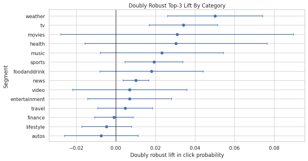
The category-level table estimates where top-rank exposure appears most or least valuable across content categories. These differences are useful for product strategy, but they should be read with uncertainty and sample-size filters in mind.
Effects By Subcategory
Subcategories are more granular than categories. They can reveal product patterns that broad categories hide. Because subcategories can be sparse, we use stricter filtering and focus on subcategories with enough treated and control rows.
Estimate Subcategory-Level Effects
This cell estimates doubly robust lift for subcategories. The result can be used to identify more specific content areas where rank position appears especially important. These estimates should be interpreted carefully because granular segments have less data.
subcategory_effects = segment_effects(model_df, "subcategory", min_rows=1_500, min_treated=75, min_control=750)
subcategory_effects.head(20)| segment_col | segment | rows | treated_rows | control_rows | treated_ctr | control_ctr | naive_lift | dr_lift | standard_error | ci_95_lower | ci_95_upper | |
|---|---|---|---|---|---|---|---|---|---|---|---|---|
| 0 | subcategory | tvnews | 2051 | 282 | 1769 | 0.2270 | 0.0543 | 0.1727 | 0.0655 | 0.0161 | 0.0339 | 0.0971 |
| 1 | subcategory | weathertopstories | 2229 | 282 | 1947 | 0.1915 | 0.0370 | 0.1545 | 0.0501 | 0.0122 | 0.0261 | 0.0741 |
| 2 | subcategory | tv-celebrity | 2665 | 214 | 2451 | 0.1776 | 0.0465 | 0.1311 | 0.0477 | 0.0168 | 0.0148 | 0.0805 |
| 3 | subcategory | restaurantsandnews | 1692 | 98 | 1594 | 0.0918 | 0.0270 | 0.0649 | 0.0460 | 0.0505 | -0.0531 | 0.1450 |
| 4 | subcategory | cma-awards | 2034 | 126 | 1908 | 0.0317 | 0.0257 | 0.0061 | 0.0294 | 0.0494 | -0.0674 | 0.1261 |
| 5 | subcategory | music-celebrity | 2460 | 342 | 2118 | 0.1959 | 0.0699 | 0.1260 | 0.0282 | 0.0151 | -0.0015 | 0.0579 |
| 6 | subcategory | traveltripideas | 2225 | 125 | 2100 | 0.0800 | 0.0214 | 0.0586 | 0.0278 | 0.0203 | -0.0120 | 0.0676 |
| 7 | subcategory | elections-2020-us | 2262 | 249 | 2013 | 0.1205 | 0.0373 | 0.0832 | 0.0271 | 0.0232 | -0.0184 | 0.0726 |
| 8 | subcategory | football_nfl | 6235 | 674 | 5561 | 0.1884 | 0.0500 | 0.1384 | 0.0251 | 0.0077 | 0.0099 | 0.0402 |
| 9 | subcategory | finance-companies | 4255 | 476 | 3779 | 0.1408 | 0.0466 | 0.0942 | 0.0247 | 0.0134 | -0.0014 | 0.0509 |
| 10 | subcategory | newscrime | 5118 | 611 | 4507 | 0.1489 | 0.0546 | 0.0944 | 0.0220 | 0.0091 | 0.0042 | 0.0397 |
| 11 | subcategory | nutrition | 2057 | 137 | 1920 | 0.0584 | 0.0234 | 0.0350 | 0.0215 | 0.0228 | -0.0232 | 0.0661 |
| 12 | subcategory | recipes | 1640 | 92 | 1548 | 0.0761 | 0.0304 | 0.0457 | 0.0205 | 0.0231 | -0.0247 | 0.0657 |
| 13 | subcategory | newsus | 12301 | 1194 | 11107 | 0.1449 | 0.0426 | 0.1023 | 0.0176 | 0.0056 | 0.0066 | 0.0287 |
| 14 | subcategory | baseball_mlb | 1537 | 107 | 1430 | 0.0654 | 0.0280 | 0.0374 | 0.0130 | 0.0206 | -0.0273 | 0.0533 |
| 15 | subcategory | shop-holidays | 2293 | 270 | 2023 | 0.0852 | 0.0262 | 0.0590 | 0.0118 | 0.0091 | -0.0061 | 0.0296 |
| 16 | subcategory | newsgoodnews | 2342 | 139 | 2203 | 0.0791 | 0.0209 | 0.0583 | 0.0105 | 0.0131 | -0.0151 | 0.0361 |
| 17 | subcategory | entertainment-celebrity | 2615 | 236 | 2379 | 0.0678 | 0.0298 | 0.0380 | 0.0056 | 0.0107 | -0.0153 | 0.0266 |
| 18 | subcategory | newsworld | 8377 | 719 | 7658 | 0.0682 | 0.0248 | 0.0433 | 0.0048 | 0.0057 | -0.0064 | 0.0161 |
| 19 | subcategory | voices | 1823 | 97 | 1726 | 0.0619 | 0.0301 | 0.0317 | 0.0046 | 0.0180 | -0.0307 | 0.0398 |
The category-level table estimates where top-rank exposure appears most or least valuable across content categories. These differences are useful for product strategy, but they should be read with uncertainty and sample-size filters in mind.
Plot Top Subcategory Effects
This plot shows the subcategories with the largest estimated doubly robust lift. This is useful for product storytelling, but it is also where multiple-comparisons risk appears. Treat these as hypotheses for deeper analysis rather than final policy recommendations.
plot_segment_effects(subcategory_effects, "Largest Doubly Robust Top-3 Lift By Subcategory", max_segments=15)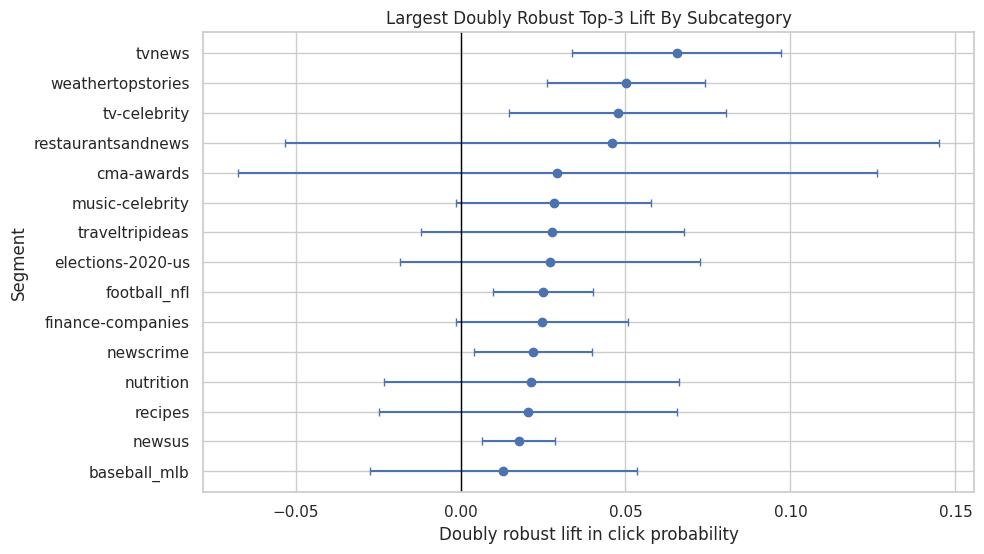
The subcategory results drill into more granular content groups. Because finer segments have smaller sample sizes, these estimates are best used to generate hypotheses rather than final policy rules on their own.
Effects By User History Depth
User history depth is a proxy for how much prior behavior the system has about the user. A rank-position effect may differ between cold-start or low-history users and users with long histories.
Estimate Effects By History Bucket
This cell estimates doubly robust top-3 lift for each user-history bucket. If low-history users show stronger effects, that could mean position matters more when personalization has less information. If high-history users show stronger effects, that could mean ranked personalization is especially effective for known users.
history_effects = segment_effects(model_df, "history_bucket", min_rows=1_000, min_treated=50, min_control=500)
history_effects| segment_col | segment | rows | treated_rows | control_rows | treated_ctr | control_ctr | naive_lift | dr_lift | standard_error | ci_95_lower | ci_95_upper | |
|---|---|---|---|---|---|---|---|---|---|---|---|---|
| 0 | history_bucket | 1-10 | 39649 | 3573 | 36076 | 0.1184 | 0.0311 | 0.0873 | 0.0168 | 0.0040 | 0.0088 | 0.0247 |
| 1 | history_bucket | 101+ | 10449 | 725 | 9724 | 0.0966 | 0.0467 | 0.0499 | 0.0103 | 0.0132 | -0.0155 | 0.0361 |
| 2 | history_bucket | 11-30 | 49100 | 3896 | 45204 | 0.1001 | 0.0325 | 0.0676 | 0.0102 | 0.0039 | 0.0025 | 0.0179 |
| 3 | history_bucket | 31-100 | 47750 | 3606 | 44144 | 0.0885 | 0.0356 | 0.0528 | 0.0080 | 0.0051 | -0.0020 | 0.0180 |
| 4 | history_bucket | 0 | 3052 | 213 | 2839 | 0.1033 | 0.0313 | 0.0719 | 0.0057 | 0.0089 | -0.0117 | 0.0231 |
The history-bucket results show whether rank exposure matters differently for users with shallow versus deep prior histories. This is directly relevant to personalization because new and experienced users may respond differently.
Plot Effects By History Bucket
This cell plots the user-history bucket estimates. The confidence intervals help distinguish meaningful differences from noise. The chart is a product-facing way to discuss whether rank position is more important for users with sparse or rich histories.
plot_segment_effects(history_effects, "Doubly Robust Top-3 Lift By User History Depth")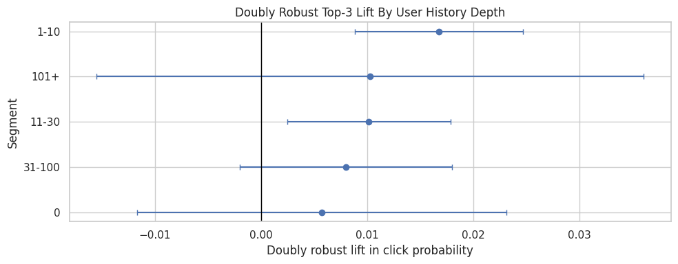
The history-bucket results show whether rank exposure matters differently for users with shallow versus deep prior histories. This is directly relevant to personalization because new and experienced users may respond differently.
Effects By Candidate Set Size
Candidate set size describes how many items appeared in the same impression. Longer lists may create more attention decay, so top-3 placement could be more valuable when users are shown many options.
Estimate Effects By Candidate Set Bucket
This cell estimates doubly robust lift for each candidate-set-size bucket. The result helps answer whether position bias is stronger in longer slates than shorter slates.
candidate_effects = segment_effects(model_df, "candidate_set_bucket", min_rows=1_000, min_treated=50, min_control=500)
candidate_effects| segment_col | segment | rows | treated_rows | control_rows | treated_ctr | control_ctr | naive_lift | dr_lift | standard_error | ci_95_lower | ci_95_upper | |
|---|---|---|---|---|---|---|---|---|---|---|---|---|
| 0 | candidate_set_bucket | 1-10 | 5865 | 3068 | 2797 | 0.2627 | 0.1376 | 0.1251 | 0.2275 | 0.0161 | 0.1959 | 0.2591 |
| 1 | candidate_set_bucket | 26-50 | 35116 | 3030 | 32086 | 0.0462 | 0.0430 | 0.0032 | 0.0142 | 0.0030 | 0.0083 | 0.0202 |
| 2 | candidate_set_bucket | 11-25 | 16951 | 2895 | 14056 | 0.0739 | 0.0706 | 0.0033 | 0.0067 | 0.0050 | -0.0030 | 0.0164 |
| 3 | candidate_set_bucket | 51-100 | 48463 | 2052 | 46411 | 0.0249 | 0.0265 | -0.0017 | 0.0022 | 0.0033 | -0.0043 | 0.0086 |
| 4 | candidate_set_bucket | 101+ | 43605 | 968 | 42637 | 0.0134 | 0.0169 | -0.0035 | -0.0088 | 0.0068 | -0.0222 | 0.0046 |
The candidate-set results check whether ranking lift changes when users face larger or smaller recommendation slates. That matters because position effects can depend on how much choice the user sees.
Plot Effects By Candidate Set Bucket
This cell visualizes the candidate-set bucket estimates. If larger slates have higher top-3 lift, that supports the idea that visibility matters more when there are many competing items.
plot_segment_effects(candidate_effects, "Doubly Robust Top-3 Lift By Candidate Set Size")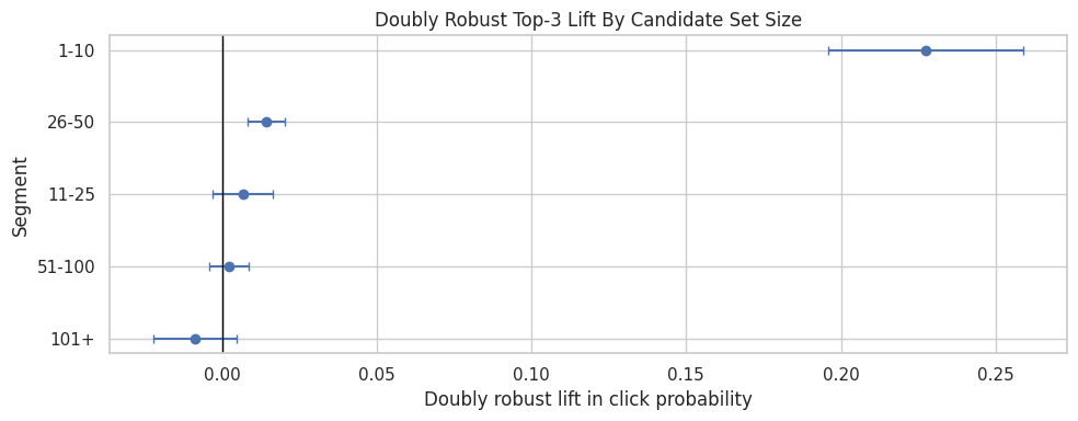
The candidate-set results check whether ranking lift changes when users face larger or smaller recommendation slates. That matters because position effects can depend on how much choice the user sees.
Effects By Item Exposure Level
Item exposure is a simple popularity/visibility proxy. The top-3 effect may differ between rarely exposed items and frequently exposed items. For example, highly exposed items may already have strong baseline demand, while lower-exposure items may depend more on prominent placement.
Estimate Effects By Exposure Quartile
This cell estimates doubly robust lift across item-exposure quartiles. Because exposure counts are skewed, quartiles are useful: each bucket has a roughly similar number of displayed rows, which keeps estimates more stable.
exposure_effects = segment_effects(model_df, "item_exposure_quartile", min_rows=1_000, min_treated=50, min_control=500)
exposure_effects| segment_col | segment | rows | treated_rows | control_rows | treated_ctr | control_ctr | naive_lift | dr_lift | standard_error | ci_95_lower | ci_95_upper | |
|---|---|---|---|---|---|---|---|---|---|---|---|---|
| 0 | item_exposure_quartile | Q4 highest | 37500 | 4525 | 32975 | 0.1421 | 0.0469 | 0.0952 | 0.0190 | 0.0032 | 0.0128 | 0.0253 |
| 1 | item_exposure_quartile | Q3 | 37500 | 3248 | 34252 | 0.0927 | 0.0343 | 0.0583 | 0.0121 | 0.0052 | 0.0018 | 0.0223 |
| 2 | item_exposure_quartile | Q2 | 37500 | 2327 | 35173 | 0.0688 | 0.0275 | 0.0412 | 0.0080 | 0.0050 | -0.0019 | 0.0179 |
| 3 | item_exposure_quartile | Q1 lowest | 37500 | 1913 | 35587 | 0.0627 | 0.0287 | 0.0341 | 0.0055 | 0.0062 | -0.0066 | 0.0176 |
The exposure-quartile results compare items with different baseline visibility. This helps separate rank effects from item popularity dynamics that may already favor highly exposed items.
Plot Effects By Exposure Quartile
This cell plots top-3 lift by exposure quartile. The result can support a product interpretation about whether prominent ranking is more useful for already-popular items or for items that otherwise receive less exposure.
plot_segment_effects(exposure_effects, "Doubly Robust Top-3 Lift By Item Exposure Quartile")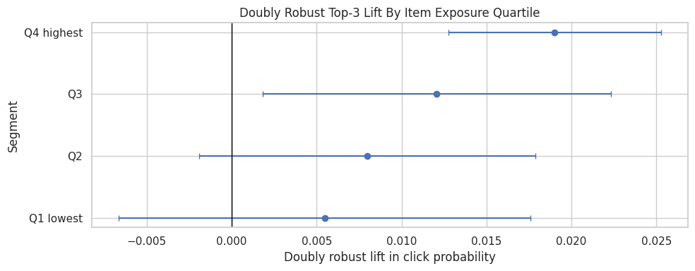
The exposure-quartile results compare items with different baseline visibility. This helps separate rank effects from item popularity dynamics that may already favor highly exposed items.
Effects By Time Of Day
User attention and browsing behavior may change throughout the day. Segmenting by time of day can reveal whether top placement matters more during certain browsing contexts.
Estimate Effects By Time Of Day
This cell estimates doubly robust top-3 lift for each time-of-day bucket. Time segments are broad enough to remain interpretable without being too sparse.
time_effects = segment_effects(model_df, "time_of_day", min_rows=1_000, min_treated=50, min_control=500)
time_effects| segment_col | segment | rows | treated_rows | control_rows | treated_ctr | control_ctr | naive_lift | dr_lift | standard_error | ci_95_lower | ci_95_upper | |
|---|---|---|---|---|---|---|---|---|---|---|---|---|
| 0 | time_of_day | afternoon | 41771 | 3354 | 38417 | 0.0987 | 0.0327 | 0.0660 | 0.0145 | 0.0049 | 0.0049 | 0.0242 |
| 1 | time_of_day | overnight | 21507 | 1552 | 19955 | 0.1108 | 0.0318 | 0.0790 | 0.0130 | 0.0061 | 0.0010 | 0.0250 |
| 2 | time_of_day | morning | 65442 | 5396 | 60046 | 0.1042 | 0.0361 | 0.0680 | 0.0108 | 0.0039 | 0.0032 | 0.0184 |
| 3 | time_of_day | late_evening | 4993 | 452 | 4541 | 0.1173 | 0.0381 | 0.0792 | 0.0100 | 0.0116 | -0.0128 | 0.0329 |
| 4 | time_of_day | evening | 16287 | 1259 | 15028 | 0.0842 | 0.0317 | 0.0525 | 0.0018 | 0.0075 | -0.0129 | 0.0165 |
The time-of-day results check whether the ranking effect changes across usage contexts. Different browsing moments can have different intent, so this is a useful product diagnostic.
Plot Effects By Time Of Day
This cell visualizes time-of-day effect estimates. Differences here can become hypotheses about user attention patterns, though time-of-day effects should be interpreted cautiously because they can correlate with content mix and user mix.
plot_segment_effects(time_effects, "Doubly Robust Top-3 Lift By Time Of Day")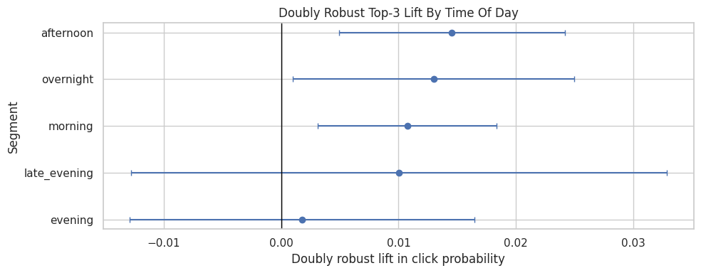
The time-of-day results check whether the ranking effect changes across usage contexts. Different browsing moments can have different intent, so this is a useful product diagnostic.
Product Summary Table
The previous sections looked at each segmentation dimension separately. This section combines all segment tables into one product summary so we can quickly see the strongest and weakest estimated effects across the notebook.
Combine Segment Results
This cell stacks all segment-effect tables and sorts them by estimated doubly robust lift. The top rows show segments where top-3 placement appears most valuable. The bottom rows show segments where estimated lift is smallest. This table is a starting point for product interpretation, not a final ranking policy.
all_effects = pd.concat(
    [
        category_effects,
        subcategory_effects,
        history_effects,
        candidate_effects,
        exposure_effects,
        time_effects,
    ],
    ignore_index=True,
)

summary_cols = [
    "segment_col",
    "segment",
    "rows",
    "treated_rows",
    "control_rows",
    "naive_lift",
    "dr_lift",
    "ci_95_lower",
    "ci_95_upper",
]

all_effects[summary_cols].sort_values("dr_lift", ascending=False).head(20)| segment_col | segment | rows | treated_rows | control_rows | naive_lift | dr_lift | ci_95_lower | ci_95_upper | |
|---|---|---|---|---|---|---|---|---|---|
| 50 | candidate_set_bucket | 1-10 | 5865 | 3068 | 2797 | 0.1251 | 0.2275 | 0.1959 | 0.2591 |
| 14 | subcategory | tvnews | 2051 | 282 | 1769 | 0.1727 | 0.0655 | 0.0339 | 0.0971 |
| 15 | subcategory | weathertopstories | 2229 | 282 | 1947 | 0.1545 | 0.0501 | 0.0261 | 0.0741 |
| 0 | category | weather | 2229 | 282 | 1947 | 0.1545 | 0.0501 | 0.0261 | 0.0741 |
| 16 | subcategory | tv-celebrity | 2665 | 214 | 2451 | 0.1311 | 0.0477 | 0.0148 | 0.0805 |
| 17 | subcategory | restaurantsandnews | 1692 | 98 | 1594 | 0.0649 | 0.0460 | -0.0531 | 0.1450 |
| 1 | category | tv | 6458 | 594 | 5864 | 0.1309 | 0.0341 | 0.0168 | 0.0515 |
| 2 | category | movies | 3442 | 249 | 3193 | 0.0420 | 0.0309 | -0.0279 | 0.0897 |
| 3 | category | health | 7739 | 442 | 7297 | 0.0170 | 0.0303 | -0.0158 | 0.0764 |
| 18 | subcategory | cma-awards | 2034 | 126 | 1908 | 0.0061 | 0.0294 | -0.0674 | 0.1261 |
| 19 | subcategory | music-celebrity | 2460 | 342 | 2118 | 0.1260 | 0.0282 | -0.0015 | 0.0579 |
| 20 | subcategory | traveltripideas | 2225 | 125 | 2100 | 0.0586 | 0.0278 | -0.0120 | 0.0676 |
| 21 | subcategory | elections-2020-us | 2262 | 249 | 2013 | 0.0832 | 0.0271 | -0.0184 | 0.0726 |
| 22 | subcategory | football_nfl | 6235 | 674 | 5561 | 0.1384 | 0.0251 | 0.0099 | 0.0402 |
| 23 | subcategory | finance-companies | 4255 | 476 | 3779 | 0.0942 | 0.0247 | -0.0014 | 0.0509 |
| 4 | category | music | 6949 | 740 | 6209 | 0.1128 | 0.0232 | -0.0079 | 0.0542 |
| 24 | subcategory | newscrime | 5118 | 611 | 4507 | 0.0944 | 0.0220 | 0.0042 | 0.0397 |
| 25 | subcategory | nutrition | 2057 | 137 | 1920 | 0.0350 | 0.0215 | -0.0232 | 0.0661 |
| 26 | subcategory | recipes | 1640 | 92 | 1548 | 0.0457 | 0.0205 | -0.0247 | 0.0657 |
| 5 | category | sports | 15075 | 1323 | 13752 | 0.1015 | 0.0192 | 0.0046 | 0.0338 |
The combined segment table creates one place to compare heterogeneous effects across dimensions. This makes it easier to identify robust high-lift segments rather than cherry-picking from separate outputs.
Inspect Segments With The Smallest Estimated Lift
This cell shows the lowest estimated segment effects. These segments may be less position-sensitive, too noisy, or poorly supported by the data. They are useful because product decisions often need to know where top placement is less incremental, not only where it helps most.
all_effects[summary_cols].sort_values("dr_lift", ascending=True).head(20)| segment_col | segment | rows | treated_rows | control_rows | naive_lift | dr_lift | ci_95_lower | ci_95_upper | |
|---|---|---|---|---|---|---|---|---|---|
| 44 | subcategory | autosenthusiasts | 1693 | 84 | 1609 | -0.0192 | -0.0297 | -0.0468 | -0.0125 |
| 43 | subcategory | markets | 3302 | 213 | 3089 | 0.0104 | -0.0148 | -0.0287 | -0.0010 |
| 42 | subcategory | lifestyleroyals | 3718 | 272 | 3446 | 0.0664 | -0.0092 | -0.0277 | 0.0093 |
| 54 | candidate_set_bucket | 101+ | 43605 | 968 | 42637 | -0.0035 | -0.0088 | -0.0222 | 0.0046 |
| 41 | subcategory | celebrity | 4296 | 310 | 3986 | 0.0216 | -0.0085 | -0.0209 | 0.0039 |
| 13 | category | autos | 7047 | 391 | 6656 | 0.0070 | -0.0074 | -0.0261 | 0.0113 |
| 40 | subcategory | football_ncaa | 1884 | 126 | 1758 | 0.0424 | -0.0064 | -0.0373 | 0.0245 |
| 39 | subcategory | foodnews | 3205 | 163 | 3042 | 0.0286 | -0.0055 | -0.0254 | 0.0145 |
| 12 | category | lifestyle | 16973 | 1264 | 15709 | 0.0328 | -0.0047 | -0.0174 | 0.0079 |
| 38 | subcategory | finance-real-estate | 2408 | 138 | 2270 | 0.0208 | -0.0044 | -0.0264 | 0.0176 |
| 37 | subcategory | autosnews | 1963 | 127 | 1836 | 0.0216 | -0.0038 | -0.0262 | 0.0186 |
| 36 | subcategory | lifestylebuzz | 3636 | 276 | 3360 | 0.0020 | -0.0032 | -0.0469 | 0.0405 |
| 11 | category | finance | 14499 | 1178 | 13321 | 0.0500 | -0.0010 | -0.0108 | 0.0087 |
| 63 | time_of_day | evening | 16287 | 1259 | 15028 | 0.0525 | 0.0018 | -0.0129 | 0.0165 |
| 53 | candidate_set_bucket | 51-100 | 48463 | 2052 | 46411 | -0.0017 | 0.0022 | -0.0043 | 0.0086 |
| 35 | subcategory | travelnews | 3079 | 204 | 2875 | 0.0744 | 0.0024 | -0.0165 | 0.0214 |
| 34 | subcategory | newspolitics | 6691 | 474 | 6217 | 0.0366 | 0.0043 | -0.0144 | 0.0229 |
| 33 | subcategory | voices | 1823 | 97 | 1726 | 0.0317 | 0.0046 | -0.0307 | 0.0398 |
| 10 | category | travel | 8220 | 482 | 7738 | 0.0495 | 0.0046 | -0.0093 | 0.0185 |
| 32 | subcategory | newsworld | 8377 | 719 | 7658 | 0.0433 | 0.0048 | -0.0064 | 0.0161 |
The low-lift segments are as important as the high-lift segments because they warn where aggressive promotion may not help. These segments are natural candidates for caution in policy simulation.
Compare Naive Lift And Doubly Robust Lift By Segment
This cell plots naive lift against doubly robust lift for all segments. Points far from the diagonal are segments where causal adjustment changed the story substantially. This is a useful diagnostic for explaining why causal adjustment matters.
plt.figure(figsize=(7, 6))
sns.scatterplot(data=all_effects, x="naive_lift", y="dr_lift", hue="segment_col", s=70)
lims = [min(all_effects["naive_lift"].min(), all_effects["dr_lift"].min()), max(all_effects["naive_lift"].max(), all_effects["dr_lift"].max())]
plt.plot(lims, lims, color="black", linestyle="--", linewidth=1)
plt.axhline(0, color="gray", linewidth=1)
plt.axvline(0, color="gray", linewidth=1)
plt.title("Naive Versus Doubly Robust Segment Lift")
plt.xlabel("Naive lift")
plt.ylabel("Doubly robust lift")
plt.tight_layout()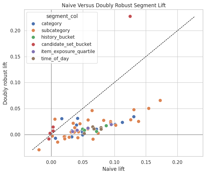
The naive lift quantifies the raw click-rate gap between treatment and control groups. It is the starting point for the project: later notebooks ask how much of this apparent lift remains after adjustment.
Interpretation Checklist
Use these questions to turn the notebook into a product narrative:
- Which broad categories have the largest adjusted top-3 lift?
- Do granular subcategories reveal stronger patterns than broad categories?
- Does rank position matter more for low-history users or high-history users?
- Does top-3 lift grow when candidate sets are larger?
- Do low-exposure or high-exposure items benefit more from top placement?
- Are any segment estimates too noisy to trust because confidence intervals are wide?
- Where does doubly robust lift differ strongly from naive lift?
A strong portfolio conclusion should sound like this:
The global top-3 effect is positive, but the estimated lift is concentrated in specific segments. This suggests that ranking-position interventions should be evaluated not only on average CTR lift, but also on where visibility creates the most incremental engagement.
Avoid overclaiming. These are observational estimates from logged recommendation data, so the final writeup should mention remaining risks: unobserved confounding, limited feature set, overlap, and the need for online experimentation to validate policy changes.