import warnings
warnings.filterwarnings("ignore")

from graphviz import Digraph
from IPython.display import Markdown, display
import matplotlib.pyplot as plt
import numpy as np
import pandas as pd
import seaborn as sns
from scipy import stats
from scipy.special import expit
import statsmodels.api as sm
import statsmodels.formula.api as smf

sns.set_theme(style="whitegrid", context="notebook")
pd.set_option("display.max_columns", 120)
pd.set_option("display.float_format", lambda x: f"{x:,.4f}")


def summarize_draws(draws, name="estimand", reference=0):
    draws = np.asarray(draws, dtype=float)
    return pd.Series(
        {
            "estimand": name,
            "mean": draws.mean(),
            "median": np.median(draws),
            "sd": draws.std(ddof=1),
            "q025": np.quantile(draws, 0.025),
            "q975": np.quantile(draws, 0.975),
            f"Pr({name} > {reference})": np.mean(draws > reference),
        }
    )


def plot_posterior(draws, title, xlabel, reference=0, decision_threshold=None, figsize=(8, 4)):
    fig, ax = plt.subplots(figsize=figsize)
    sns.histplot(draws, bins=55, kde=True, color="#9ecae1", ax=ax)
    ax.axvline(reference, color="#444444", linestyle="--", linewidth=1, label=f"Reference = {reference:g}")
    if decision_threshold is not None:
        ax.axvline(decision_threshold, color="#de2d26", linestyle=":", linewidth=2, label=f"Decision threshold = {decision_threshold:g}")
    ax.set_title(title)
    ax.set_xlabel(xlabel)
    ax.set_ylabel("Posterior draws")
    ax.legend()
    plt.tight_layout()
    return fig, ax


def plot_interval_table(table, title, xlabel, reference=0, figsize=(8.5, 4.5)):
    plot_df = table.copy().sort_values("mean")
    fig, ax = plt.subplots(figsize=figsize)
    ax.errorbar(
        x=plot_df["mean"],
        y=plot_df.index,
        xerr=[
            plot_df["mean"] - plot_df["q025"],
            plot_df["q975"] - plot_df["mean"],
        ],
        fmt="o",
        color="#2b8cbe",
        ecolor="#a6bddb",
        elinewidth=3,
        capsize=4,
    )
    ax.axvline(reference, color="#444444", linestyle="--", linewidth=1)
    ax.set_title(title)
    ax.set_xlabel(xlabel)
    ax.set_ylabel("")
    plt.tight_layout()
return fig, ax09. Bayesian Causal Inference
Bayesian causal inference is not a different definition of causality. It is a probabilistic way to reason about causal estimands, uncertainty, prior information, heterogeneity, missing potential outcomes, and decisions.
The causal part still comes from design:
- What is the intervention?
- What is the estimand?
- Why are treatment groups exchangeable?
- What variables must be adjusted for?
- What assumptions identify the missing potential outcomes?
The Bayesian part gives a coherent way to express uncertainty after those design choices:
\[ p(\text{causal estimand} \mid \text{data}, \text{model}, \text{assumptions}) \]
This notebook builds Bayesian causal analyses from small pieces: Bayesian A/B testing, posterior treatment effects, Bayesian regression adjustment, prior sensitivity, hierarchical treatment effects, causal impact with counterfactual forecasting, and decision analysis.
Learning Goals
By the end of this notebook, you should be able to:
- Explain how Bayesian inference fits into the potential outcomes framework.
- Compute posterior distributions for treatment effects in randomized experiments.
- Interpret posterior probabilities, credible intervals, and decision probabilities.
- Use Bayesian regression adjustment for causal effects under exchangeability assumptions.
- Explain why Bayesian modeling does not fix unmeasured confounding by itself.
- Use hierarchical shrinkage to stabilize segment-level treatment effects.
- Run prior sensitivity analysis for small experiments.
- Build a lightweight Bayesian causal-impact analysis using pre-period controls.
- Translate posterior causal uncertainty into expected business value and launch decisions.
1. Setup
We will use numpy, pandas, scipy, statsmodels, seaborn, matplotlib, and Graphviz. The examples use direct posterior simulation rather than heavyweight probabilistic programming so that the notebook remains portable for the website.
2. Bayesian Inference and Potential Outcomes
For each unit, the potential outcomes are:
\[ Y_i(1), \quad Y_i(0) \]
The individual causal effect is:
\[ Y_i(1) - Y_i(0) \]
but we observe only one potential outcome per unit:
\[ Y_i = A_iY_i(1) + (1-A_i)Y_i(0) \]
Bayesian causal inference treats missing potential outcomes and causal estimands as uncertain quantities. A posterior distribution for the average treatment effect might be written:
\[ p\left(ATE \mid Y^{obs}, A, X\right) \]
where the identification assumptions still matter. Bayesian updating does not remove the need for exchangeability, positivity, consistency, and correct measurement.
dot = Digraph("bayesian_causal_pipeline", graph_attr={"rankdir": "LR"})
dot.attr("node", shape="box", style="rounded,filled", fillcolor="#f7fbff", color="#6baed6")

dot.node("Design", "Causal design\nidentification assumptions")
dot.node("Prior", "Prior information\nskepticism, constraints")
dot.node("Likelihood", "Likelihood\noutcome model")
dot.node("Posterior", "Posterior over\ncausal estimands")
dot.node("Decision", "Decision analysis\nexpected utility")

dot.edge("Design", "Likelihood")
dot.edge("Prior", "Posterior")
dot.edge("Likelihood", "Posterior")
dot.edge("Posterior", "Decision")

dot
Rubin (1978) is a classic Bayesian treatment of causal effects and randomization. The modern Bayesian causal toolkit includes regression adjustment, Bayesian nonparametrics such as BART, Bayesian causal forests, hierarchical models, and Bayesian structural time-series models.
3. Bayesian A/B Test for a Binary Outcome
Start with a randomized product experiment.
Treatment is randomized, so the causal design is simple:
\[ A \perp (Y(1), Y(0)) \]
For binary conversion outcomes:
\[ Y_i(a) \sim Bernoulli(p_a) \]
Use a beta prior:
\[ p_a \sim Beta(\alpha_a, \beta_a) \]
The posterior is:
\[ p_a \mid data \sim Beta(\alpha_a + y_a,\ \beta_a + n_a - y_a) \]
The treatment effect can be represented by posterior draws:
\[ \Delta = p_1 - p_0 \]
rng = np.random.default_rng(4909)
n_control = 5200
n_treated = 5100
true_p0 = 0.118
true_p1 = 0.129

y_control = rng.binomial(n_control, true_p0)
y_treated = rng.binomial(n_treated, true_p1)

alpha0, beta0 = 1, 1
posterior_control = (alpha0 + y_control, beta0 + n_control - y_control)
posterior_treated = (alpha0 + y_treated, beta0 + n_treated - y_treated)

draws = 80_000
p0_draws = rng.beta(*posterior_control, size=draws)
p1_draws = rng.beta(*posterior_treated, size=draws)
lift_draws = p1_draws - p0_draws
relative_lift_draws = lift_draws / p0_draws

ab_summary = pd.DataFrame(
    [
        summarize_draws(p0_draws, "p_control"),
        summarize_draws(p1_draws, "p_treated"),
        summarize_draws(lift_draws, "absolute_lift"),
        summarize_draws(relative_lift_draws, "relative_lift"),
    ]
)

experiment_counts = pd.DataFrame(
    {
        "arm": ["Control", "Treatment"],
        "n": [n_control, n_treated],
        "conversions": [y_control, y_treated],
        "observed_rate": [y_control / n_control, y_treated / n_treated],
    }
)

experiment_counts, ab_summary
( arm n conversions observed_rate
0 Control 5200 593 0.1140
1 Treatment 5100 635 0.1245,
estimand mean median sd q025 q975 Pr(p_control > 0) \
0 p_control 0.1142 0.1141 0.0044 0.1057 0.1230 1.0000
1 p_treated 0.1247 0.1246 0.0046 0.1157 0.1338 NaN
2 absolute_lift 0.0105 0.0105 0.0064 -0.0021 0.0229 NaN
3 relative_lift 0.0934 0.0918 0.0585 -0.0175 0.2118 NaN
Pr(p_treated > 0) Pr(absolute_lift > 0) Pr(relative_lift > 0)
0 NaN NaN NaN
1 1.0000 NaN NaN
2 NaN 0.9487 NaN
3 NaN NaN 0.9487 )plot_posterior(
lift_draws,
title="Posterior distribution of absolute conversion lift",
xlabel="Treatment conversion rate minus control conversion rate",
reference=0,
decision_threshold=0.005,
)
plt.show()
pd.Series(
{
"Pr(lift > 0)": np.mean(lift_draws > 0),
"Pr(lift > 0.5 percentage points)": np.mean(lift_draws > 0.005),
"Pr(relative lift > 5%)": np.mean(relative_lift_draws > 0.05),
}
)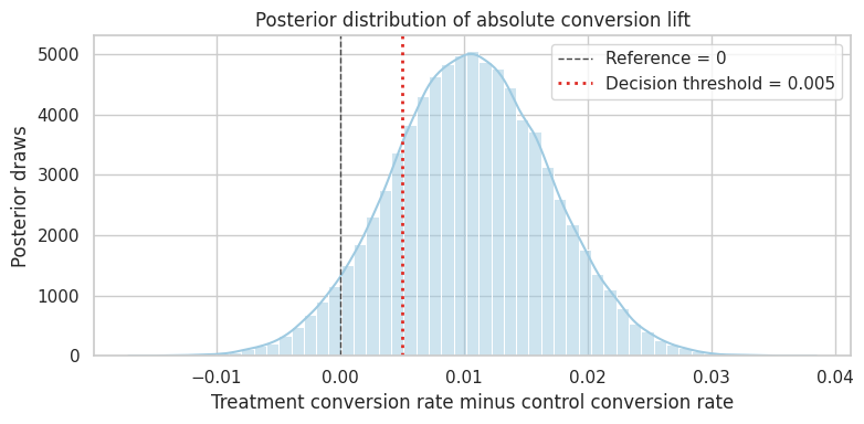
Pr(lift > 0)                       0.9487
Pr(lift > 0.5 percentage points)   0.8062
Pr(relative lift > 5%)             0.7682
dtype: float64
Interpretation
The posterior answers decision-oriented questions directly:
- What is the probability the lift is positive?
- What is the probability it exceeds a practical threshold?
- How large is the downside risk?
This is often easier to communicate than only reporting a p-value. But the result is still conditional on the causal design and the model.
4. Prior Sensitivity in Small Experiments
With large experiments, weak priors usually have little impact. With small experiments, priors matter.
Let us compare:
- a weak uniform prior,
- a mildly skeptical prior centered around a 10% conversion rate,
- an optimistic prior expecting the treatment to improve conversion.
rng = np.random.default_rng(4910)
small_n_control = 180
small_n_treated = 175
small_y_control = rng.binomial(small_n_control, 0.10)
small_y_treated = rng.binomial(small_n_treated, 0.125)

prior_specs = {
    "Weak uniform": {"control": (1, 1), "treated": (1, 1)},
    "Skeptical around 10%": {"control": (20, 180), "treated": (20, 180)},
    "Optimistic treatment prior": {"control": (20, 180), "treated": (28, 172)},
}

prior_rows = []
prior_draws = {}
for prior_name, spec in prior_specs.items():
    c_post = (
        spec["control"][0] + small_y_control,
        spec["control"][1] + small_n_control - small_y_control,
    )
    t_post = (
        spec["treated"][0] + small_y_treated,
        spec["treated"][1] + small_n_treated - small_y_treated,
    )
    c_draw = rng.beta(*c_post, size=60_000)
    t_draw = rng.beta(*t_post, size=60_000)
    effect = t_draw - c_draw
    prior_draws[prior_name] = effect
    row = summarize_draws(effect, "lift")
    row["prior"] = prior_name
    prior_rows.append(row)

prior_sensitivity = pd.DataFrame(prior_rows).set_index("prior")
pd.Series(
    {
        "small_control_conversions": small_y_control,
        "small_treated_conversions": small_y_treated,
        "small_control_rate": small_y_control / small_n_control,
        "small_treated_rate": small_y_treated / small_n_treated,
    }
), prior_sensitivity
(small_control_conversions 22.0000
small_treated_conversions 23.0000
small_control_rate 0.1222
small_treated_rate 0.1314
dtype: float64,
estimand mean median sd q025 q975 \
prior
Weak uniform lift 0.0092 0.0093 0.0356 -0.0614 0.0791
Skeptical around 10% lift 0.0041 0.0042 0.0229 -0.0407 0.0490
Optimistic treatment prior lift 0.0254 0.0255 0.0239 -0.0213 0.0723
Pr(lift > 0)
prior
Weak uniform 0.6035
Skeptical around 10% 0.5721
Optimistic treatment prior 0.8560 )fig, ax = plt.subplots(figsize=(8, 4.5))
for prior_name, effect in prior_draws.items():
sns.kdeplot(effect, ax=ax, label=prior_name)
ax.axvline(0, color="#444444", linestyle="--", linewidth=1)
ax.set_title("Small experiments can be prior-sensitive")
ax.set_xlabel("Absolute conversion lift")
ax.set_ylabel("Posterior density")
ax.legend()
plt.tight_layout()
plt.show()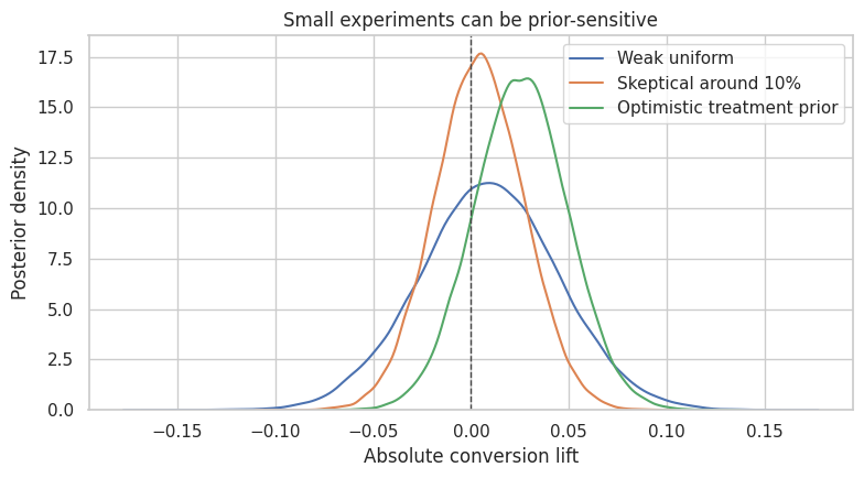
Practical Rule
Prior sensitivity is not a weakness to hide. It is information.
If a decision changes depending on a plausible prior, say that the experiment is not decisive. The professional response is usually one of:
- collect more data,
- use stronger historical evidence,
- narrow the decision threshold,
- make a reversible low-risk decision,
- explicitly price the uncertainty.
5. Bayesian Continuous-Outcome Experiment
For a continuous outcome, we can model each arm with a normal likelihood:
\[ Y_i(a) \sim Normal(\mu_a, \sigma_a^2) \]
Using a weak normal-inverse-gamma prior, we can sample from the posterior of each arm’s mean and form:
\[ \Delta = \mu_1 - \mu_0 \]
def normal_inverse_gamma_posterior_draws(y, draws=50_000, mu0=0, kappa0=1e-4, alpha0=1e-3, beta0=1e-3, rng=None):
    if rng is None:
        rng = np.random.default_rng()
    y = np.asarray(y, dtype=float)
    n = len(y)
    ybar = y.mean()
    ss = np.sum((y - ybar) ** 2)
    kappa_n = kappa0 + n
    mu_n = (kappa0 * mu0 + n * ybar) / kappa_n
    alpha_n = alpha0 + n / 2
    beta_n = beta0 + 0.5 * ss + (kappa0 * n * (ybar - mu0) ** 2) / (2 * kappa_n)
    sigma2 = stats.invgamma.rvs(a=alpha_n, scale=beta_n, size=draws, random_state=rng)
    mu = rng.normal(mu_n, np.sqrt(sigma2 / kappa_n))
    return mu, sigma2


rng = np.random.default_rng(4911)
n = 1400
df_exp = pd.DataFrame({"A": rng.binomial(1, 0.5, size=n)})
df_exp["pre_value"] = rng.normal(0, 1, size=n)
true_continuous_effect = 1.25
df_exp["Y"] = (
    20
    + true_continuous_effect * df_exp["A"]
    + 2.5 * df_exp["pre_value"]
    + rng.normal(0, 6, size=n)
)

mu0_draw, _ = normal_inverse_gamma_posterior_draws(df_exp.loc[df_exp["A"] == 0, "Y"], rng=rng)
mu1_draw, _ = normal_inverse_gamma_posterior_draws(df_exp.loc[df_exp["A"] == 1, "Y"], rng=rng)
continuous_effect_draws = mu1_draw - mu0_draw

continuous_summary = summarize_draws(continuous_effect_draws, "mean_difference")
continuous_summary
estimand mean_difference
mean 1.3457
median 1.3454
sd 0.3393
q025 0.6827
q975 2.0118
Pr(mean_difference > 0) 0.9999
dtype: objectplot_posterior(
continuous_effect_draws,
title="Posterior treatment effect for a continuous outcome",
xlabel="Mean treatment-control difference",
reference=0,
decision_threshold=1.0,
)
plt.show()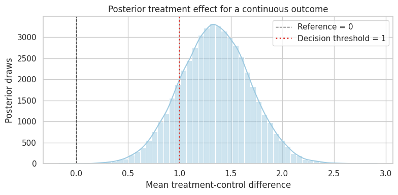
This posterior is based on a randomized experiment. We do not need to model treatment assignment to identify the effect. The Bayesian model summarizes uncertainty about the arm means and their difference.
6. Bayesian Regression Adjustment
Regression adjustment can improve precision and estimate conditional effects.
Assume:
\[ Y_i = X_i^\top\beta + \epsilon_i \]
with:
\[ \epsilon_i \sim Normal(0, \sigma^2) \]
and a conjugate prior:
\[ \beta \mid \sigma^2 \sim Normal(\beta_0, \sigma^2 V_0) \]
\[ \sigma^2 \sim InvGamma(a_0, b_0) \]
The treatment coefficient posterior gives a regression-adjusted causal effect in a randomized experiment, assuming the model is adequate for the adjustment target.
def bayesian_linear_regression_draws(X, y, draws=50_000, beta0=None, V0_scale=1e6, a0=1e-3, b0=1e-3, rng=None):
    if rng is None:
        rng = np.random.default_rng()
    X = np.asarray(X, dtype=float)
    y = np.asarray(y, dtype=float)
    n, p = X.shape
    if beta0 is None:
        beta0 = np.zeros(p)
    beta0 = np.asarray(beta0, dtype=float)
    V0_inv = np.eye(p) / V0_scale
    Vn = np.linalg.inv(V0_inv + X.T @ X)
    beta_n = Vn @ (V0_inv @ beta0 + X.T @ y)
    a_n = a0 + n / 2
    residual_part = y.T @ y + beta0.T @ V0_inv @ beta0 - beta_n.T @ np.linalg.inv(Vn) @ beta_n
    b_n = b0 + 0.5 * residual_part
    sigma2_draws = stats.invgamma.rvs(a=a_n, scale=b_n, size=draws, random_state=rng)
    beta_draws = np.empty((draws, p))
    chol = np.linalg.cholesky(Vn)
    z = rng.normal(size=(draws, p))
    for i in range(draws):
        beta_draws[i] = beta_n + np.sqrt(sigma2_draws[i]) * (chol @ z[i])
    return beta_draws, sigma2_draws


X = sm.add_constant(df_exp[["A", "pre_value"]]).to_numpy()
y = df_exp["Y"].to_numpy()
beta_draws, sigma2_draws = bayesian_linear_regression_draws(X, y, draws=50_000, rng=rng)
regression_effect_draws = beta_draws[:, 1]

adjusted_summary = pd.DataFrame(
    [
        summarize_draws(continuous_effect_draws, "unadjusted_mean_difference"),
        summarize_draws(regression_effect_draws, "regression_adjusted_effect"),
    ]
).set_index("estimand")

adjusted_summary| mean | median | sd | q025 | q975 | Pr(unadjusted_mean_difference > 0) | Pr(regression_adjusted_effect > 0) | |
|---|---|---|---|---|---|---|---|
| estimand | |||||||
| unadjusted_mean_difference | 1.3457 | 1.3454 | 0.3393 | 0.6827 | 2.0118 | 0.9999 | NaN |
| regression_adjusted_effect | 1.0392 | 1.0407 | 0.3125 | 0.4243 | 1.6511 | NaN | 0.9995 |
plot_interval_table(
    adjusted_summary,
    title="Regression adjustment reduces posterior uncertainty in this randomized experiment",
    xlabel="Treatment effect",
    reference=true_continuous_effect,
    figsize=(8, 3.6),
)
plt.show()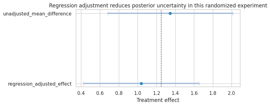
The regression-adjusted posterior is narrower because pre_value is strongly predictive of the outcome. Randomization identifies the effect; regression uses baseline information to improve precision.
7. Bayesian Modeling Does Not Fix Unmeasured Confounding
Bayesian regression can adjust for measured covariates. It cannot magically adjust for variables omitted from the model.
Now simulate observational treatment assignment:
\[ P(A=1 \mid X, U) \]
where \(U\) is unobserved in the analyst’s dataset and affects \(Y\).
rng = np.random.default_rng(4912)
n = 4500
obs = pd.DataFrame(
    {
        "X": rng.normal(size=n),
        "U": rng.normal(size=n),
    }
)
true_obs_effect = 1.0
obs["A"] = rng.binomial(1, expit(-0.2 + 1.0 * obs["X"] + 1.1 * obs["U"]), size=n)
obs["Y"] = 5 + true_obs_effect * obs["A"] + 1.4 * obs["X"] + 2.0 * obs["U"] + rng.normal(0, 1.4, size=n)

def posterior_treatment_coef(data, predictors, draws=40_000):
    Xmat = sm.add_constant(data[predictors]).to_numpy()
    beta, _ = bayesian_linear_regression_draws(Xmat, data["Y"].to_numpy(), draws=draws, rng=rng)
    treatment_index = ["const"] + predictors
    return beta[:, treatment_index.index("A")]


unadjusted_draws = posterior_treatment_coef(obs, ["A"])
adjust_x_draws = posterior_treatment_coef(obs, ["A", "X"])
oracle_draws = posterior_treatment_coef(obs, ["A", "X", "U"])

confounding_summary = pd.DataFrame(
    [
        summarize_draws(unadjusted_draws, "Unadjusted"),
        summarize_draws(adjust_x_draws, "Adjust for observed X"),
        summarize_draws(oracle_draws, "Oracle adjust for X and U"),
    ]
).set_index("estimand")

confounding_summary| mean | median | sd | q025 | q975 | Pr(Unadjusted > 0) | Pr(Adjust for observed X > 0) | Pr(Oracle adjust for X and U > 0) | |
|---|---|---|---|---|---|---|---|---|
| estimand | ||||||||
| Unadjusted | 3.5657 | 3.5656 | 0.0752 | 3.4178 | 3.7118 | 1.0000 | NaN | NaN |
| Adjust for observed X | 2.7790 | 2.7790 | 0.0730 | 2.6366 | 2.9217 | NaN | 1.0000 | NaN |
| Oracle adjust for X and U | 0.9355 | 0.9353 | 0.0491 | 0.8396 | 1.0315 | NaN | NaN | 1.0000 |
plot_interval_table(
    confounding_summary,
    title="Bayesian regression still needs the right adjustment set",
    xlabel="Posterior treatment coefficient",
    reference=true_obs_effect,
    figsize=(8, 4.2),
)
plt.show()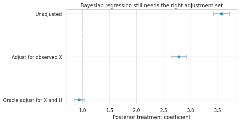
Interpretation
The posterior intervals can be narrow and still centered on the wrong estimand. This is an important distinction:
- Bayesian inference quantifies uncertainty under the model.
- Causal identification decides whether the model targets the causal estimand.
Unmeasured confounding is not solved by adding a prior to an otherwise misspecified causal model.
8. Prior Over Bias: Sensitivity Analysis
One Bayesian way to handle unmeasured confounding is to place a prior over the bias.
Suppose the adjusted estimate is:
\[ \widehat{\tau}_{obs} \]
but we believe unmeasured confounding may bias it upward by \(B\):
\[ \tau = \widehat{\tau}_{obs} - B \]
We can assign a prior to \(B\) and propagate that uncertainty.
rng = np.random.default_rng(4913)
observed_effect_draws = adjust_x_draws

bias_scenarios = {
    "No extra confounding": rng.normal(0.0, 0.05, size=len(observed_effect_draws)),
    "Moderate upward bias": rng.normal(0.6, 0.25, size=len(observed_effect_draws)),
    "Large uncertain upward bias": rng.normal(1.1, 0.50, size=len(observed_effect_draws)),
}

bias_rows = []
bias_adjusted_draws = {}
for scenario, bias_draw in bias_scenarios.items():
    adjusted = observed_effect_draws - bias_draw
    bias_adjusted_draws[scenario] = adjusted
    row = summarize_draws(adjusted, scenario)
    bias_rows.append(row)

bias_sensitivity = pd.DataFrame(bias_rows).set_index("estimand")
bias_sensitivity| mean | median | sd | q025 | q975 | Pr(No extra confounding > 0) | Pr(Moderate upward bias > 0) | Pr(Large uncertain upward bias > 0) | |
|---|---|---|---|---|---|---|---|---|
| estimand | ||||||||
| No extra confounding | 2.7786 | 2.7786 | 0.0887 | 2.6064 | 2.9528 | 1.0000 | NaN | NaN |
| Moderate upward bias | 2.1776 | 2.1769 | 0.2622 | 1.6675 | 2.6924 | NaN | 1.0000 | NaN |
| Large uncertain upward bias | 1.6805 | 1.6826 | 0.5068 | 0.6717 | 2.6694 | NaN | NaN | 0.9996 |
fig, ax = plt.subplots(figsize=(8.5, 4.5))
for scenario, draws_ in bias_adjusted_draws.items():
    sns.kdeplot(draws_, ax=ax, label=scenario)
ax.axvline(0, color="#444444", linestyle="--", linewidth=1)
ax.axvline(true_obs_effect, color="#31a354", linestyle=":", linewidth=2, label="True effect in simulation")
ax.set_title("Bias priors translate unmeasured confounding into causal uncertainty")
ax.set_xlabel("Bias-adjusted causal effect")
ax.set_ylabel("Posterior density")
ax.legend()
plt.tight_layout()
plt.show()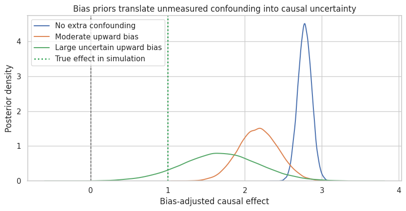
This approach is honest because it separates two uncertainties:
- posterior uncertainty from the fitted outcome model,
- causal uncertainty from unmeasured confounding.
The second uncertainty is not learned from the observed outcome regression alone. It comes from external knowledge, design judgment, negative controls, validation data, or sensitivity assumptions.
9. Hierarchical Treatment Effects Across Segments
Industry teams often want treatment effects by segment:
- region,
- customer tier,
- acquisition channel,
- product category,
- sales team,
- hospital,
- school.
Segment estimates are noisy when some segments are small. Hierarchical Bayesian models partially pool segment effects:
\[ \widehat{\tau}_j \sim Normal(\tau_j, s_j^2) \]
\[ \tau_j \sim Normal(\mu, \omega^2) \]
The posterior mean for segment \(j\) is a precision-weighted average of the noisy segment estimate and the overall mean.
rng = np.random.default_rng(4914)
n_segments = 18
segment_sizes = rng.integers(80, 700, size=n_segments)
true_mu = 1.2
true_omega = 0.75

segment_rows = []
for j, size in enumerate(segment_sizes):
    true_tau_j = rng.normal(true_mu, true_omega)
    A = rng.binomial(1, 0.5, size=size)
    baseline = rng.normal(0, 1, size=size)
    Y = 10 + true_tau_j * A + 1.5 * baseline + rng.normal(0, 3.0, size=size)
    tmp = pd.DataFrame({"segment": f"S{j+1:02d}", "A": A, "baseline": baseline, "Y": Y, "true_tau": true_tau_j})
    segment_rows.append(tmp)

seg_df = pd.concat(segment_rows, ignore_index=True)

raw_rows = []
for segment, part in seg_df.groupby("segment"):
    model = smf.ols("Y ~ A + baseline", data=part).fit()
    raw_rows.append(
        {
            "segment": segment,
            "n": len(part),
            "raw_estimate": model.params["A"],
            "raw_se": model.bse["A"],
            "true_tau": part["true_tau"].iloc[0],
        }
    )

seg_est = pd.DataFrame(raw_rows)
mu_hat = np.average(seg_est["raw_estimate"], weights=1 / seg_est["raw_se"] ** 2)
between_var_hat = max(
    0.05,
    np.var(seg_est["raw_estimate"], ddof=1) - np.mean(seg_est["raw_se"] ** 2),
)
omega_hat = np.sqrt(between_var_hat)

prior_precision = 1 / omega_hat**2
data_precision = 1 / seg_est["raw_se"] ** 2
seg_est["shrunk_estimate"] = (
    data_precision * seg_est["raw_estimate"] + prior_precision * mu_hat
) / (data_precision + prior_precision)
seg_est["shrinkage_weight_on_raw"] = data_precision / (data_precision + prior_precision)

seg_est.sort_values("n").head(8), pd.Series({"overall_mu_hat": mu_hat, "omega_hat": omega_hat})
( segment n raw_estimate raw_se true_tau shrunk_estimate \
16 S17 120 1.6314 0.5140 1.4138 1.4284
15 S16 125 0.5686 0.5014 0.0904 0.7804
11 S12 241 1.6945 0.3672 1.0353 1.5502
10 S11 272 0.8079 0.3668 1.4261 0.8860
6 S07 288 -0.3294 0.3796 0.0723 0.0528
13 S14 362 1.0500 0.3185 0.7231 1.0640
14 S15 372 2.1028 0.2928 2.0549 1.9301
2 S03 377 1.4725 0.3064 0.9251 1.4057
shrinkage_weight_on_raw
16 0.6036
15 0.6154
11 0.7490
10 0.7494
6 0.7362
13 0.7986
14 0.8243
2 0.8108 ,
overall_mu_hat 1.1195
omega_hat 0.6343
dtype: float64)fig, axes = plt.subplots(1, 2, figsize=(13, 5))
plot_df = seg_est.sort_values("n")
axes[0].scatter(plot_df["raw_estimate"], plot_df["segment"], s=40 + plot_df["n"] / 12, label="Raw", color="#9ecae1")
axes[0].scatter(plot_df["shrunk_estimate"], plot_df["segment"], s=40 + plot_df["n"] / 12, label="Partially pooled", color="#2b8cbe")
for _, row in plot_df.iterrows():
axes[0].plot([row["raw_estimate"], row["shrunk_estimate"]], [row["segment"], row["segment"]], color="#bbbbbb", linewidth=1)
axes[0].axvline(mu_hat, color="#444444", linestyle="--", linewidth=1, label="Overall mean")
axes[0].set_title("Hierarchical shrinkage stabilizes segment effects")
axes[0].set_xlabel("Treatment effect")
axes[0].set_ylabel("Segment")
axes[0].legend()
sns.scatterplot(data=seg_est, x="n", y="shrinkage_weight_on_raw", ax=axes[1], color="#2b8cbe")
axes[1].set_title("Small segments borrow more strength")
axes[1].set_xlabel("Segment sample size")
axes[1].set_ylabel("Weight on raw segment estimate")
plt.tight_layout()
plt.show()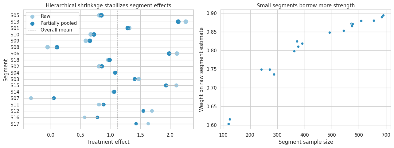
Interpretation
Small, noisy segment estimates are pulled more strongly toward the overall mean. Large segments keep more of their own signal.
This is one reason Bayesian hierarchical models are common in applied causal work: they allow heterogeneous effects without treating every tiny subgroup estimate as equally reliable.
10. Bayesian Causal Impact with Counterfactual Forecasting
For market-level interventions, we may have one treated time series and one or more control series. A Bayesian structural time-series model predicts the counterfactual post-treatment outcome using pre-treatment relationships.
Here we build a lightweight version:
- Fit a Bayesian regression of treated-market outcome on control-market outcomes in the pre-period.
- Draw posterior regression coefficients.
- Predict the post-period counterfactual.
- Compare observed post-period outcomes with posterior counterfactual draws.
rng = np.random.default_rng(4915)
T = 120
intervention_time = 82
time = np.arange(T)

control_1 = 40 + 0.22 * time + 3.0 * np.sin(time / 8) + rng.normal(0, 1.5, size=T)
control_2 = 28 + 0.15 * time + 2.0 * np.cos(time / 10) + rng.normal(0, 1.4, size=T)
baseline_treated = 8 + 0.58 * control_1 + 0.42 * control_2 + rng.normal(0, 1.8, size=T)
true_impact = np.where(time >= intervention_time, 4.5 + 0.05 * (time - intervention_time), 0.0)
treated_series = baseline_treated + true_impact

ts_df = pd.DataFrame(
    {
        "time": time,
        "treated_market": treated_series,
        "control_1": control_1,
        "control_2": control_2,
        "post": (time >= intervention_time).astype(int),
        "true_impact": true_impact,
    }
)

pre = ts_df.loc[ts_df["post"] == 0].copy()
post = ts_df.loc[ts_df["post"] == 1].copy()

X_pre = sm.add_constant(pre[["control_1", "control_2", "time"]]).to_numpy()
y_pre = pre["treated_market"].to_numpy()
beta_ts_draws, sigma2_ts_draws = bayesian_linear_regression_draws(X_pre, y_pre, draws=30_000, V0_scale=1e4, rng=rng)

X_all = sm.add_constant(ts_df[["control_1", "control_2", "time"]]).to_numpy()
counterfactual_mean_draws = beta_ts_draws @ X_all.T
noise_draws = rng.normal(0, np.sqrt(sigma2_ts_draws[:, None]), size=counterfactual_mean_draws.shape)
counterfactual_draws = counterfactual_mean_draws + noise_draws

post_counterfactual = counterfactual_draws[:, ts_df["post"].to_numpy() == 1]
post_observed = post["treated_market"].to_numpy()
pointwise_impact_draws = post_observed[None, :] - post_counterfactual
cumulative_impact_draws = pointwise_impact_draws.sum(axis=1)
average_impact_draws = pointwise_impact_draws.mean(axis=1)

impact_summary = pd.DataFrame(
    [
        summarize_draws(average_impact_draws, "average_post_period_impact"),
        summarize_draws(cumulative_impact_draws, "cumulative_post_period_impact"),
    ]
)

impact_summary| estimand | mean | median | sd | q025 | q975 | Pr(average_post_period_impact > 0) | Pr(cumulative_post_period_impact > 0) | |
|---|---|---|---|---|---|---|---|---|
| 0 | average_post_period_impact | 6.0009 | 5.9963 | 0.6247 | 4.7789 | 7.2381 | 1.0000 | NaN |
| 1 | cumulative_post_period_impact | 228.0353 | 227.8600 | 23.7377 | 181.5990 | 275.0475 | NaN | 1.0000 |
cf_mean = counterfactual_draws.mean(axis=0)
cf_low = np.quantile(counterfactual_draws, 0.025, axis=0)
cf_high = np.quantile(counterfactual_draws, 0.975, axis=0)

fig, axes = plt.subplots(2, 1, figsize=(10, 7), sharex=True)

axes[0].plot(ts_df["time"], ts_df["treated_market"], label="Observed treated market", color="#2b8cbe")
axes[0].plot(ts_df["time"], cf_mean, label="Posterior counterfactual mean", color="#444444")
axes[0].fill_between(ts_df["time"], cf_low, cf_high, color="#bdbdbd", alpha=0.35, label="95% posterior interval")
axes[0].axvline(intervention_time, color="#de2d26", linestyle="--", linewidth=1)
axes[0].set_title("Bayesian counterfactual forecast for causal impact")
axes[0].set_ylabel("Outcome")
axes[0].legend()

impact_mean = pointwise_impact_draws.mean(axis=0)
impact_low = np.quantile(pointwise_impact_draws, 0.025, axis=0)
impact_high = np.quantile(pointwise_impact_draws, 0.975, axis=0)
axes[1].plot(post["time"], impact_mean, color="#2b8cbe", label="Pointwise impact")
axes[1].fill_between(post["time"], impact_low, impact_high, color="#9ecae1", alpha=0.45)
axes[1].axhline(0, color="#444444", linewidth=1)
axes[1].set_title("Posterior pointwise impact")
axes[1].set_xlabel("Time")
axes[1].set_ylabel("Observed minus counterfactual")

plt.tight_layout()
plt.show()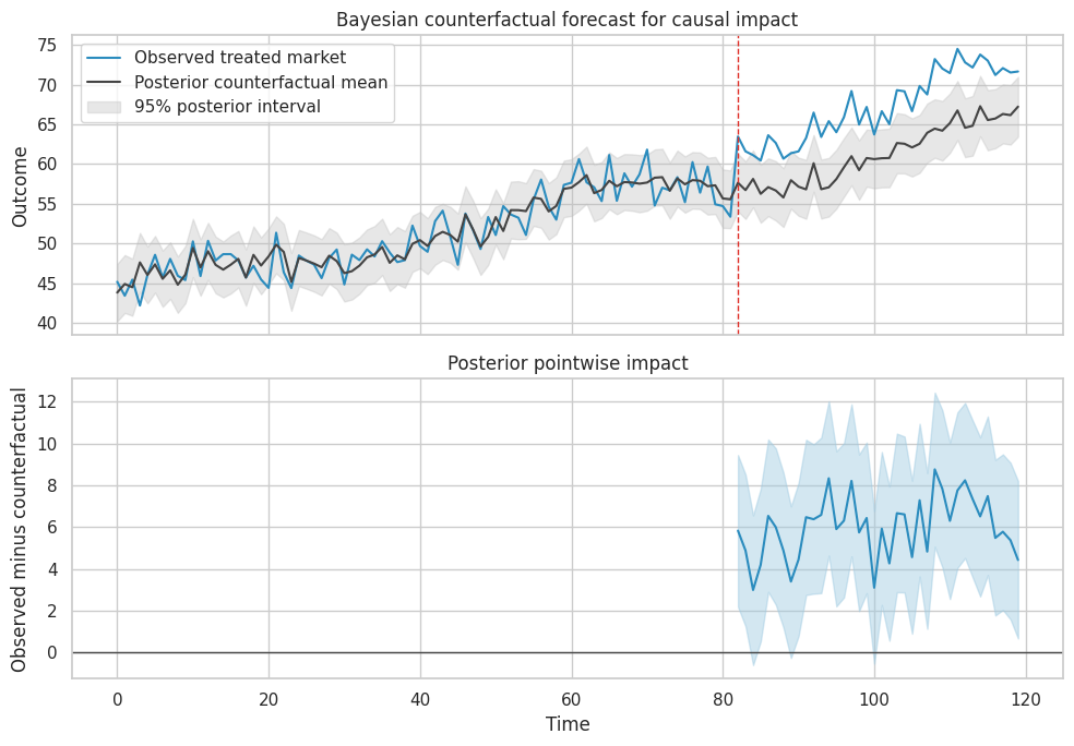
Causal Caveat
The time-series posterior is causal only if the controls represent what would have happened to the treated market absent intervention.
The method can fail if:
- control markets are affected by the intervention,
- the treated market was already diverging before treatment,
- post-period shocks hit only the treated market,
- the intervention changes measurement,
- the pre-period relationship is unstable.
11. Bayesian Decision Analysis
Bayesian causal inference is naturally connected to decisions.
Suppose the product intervention from the A/B test creates value per additional conversion, but launch has implementation cost and possible downside cost.
For each posterior draw, compute profit:
\[ Profit = Users \times Lift \times ValuePerConversion - Cost \]
Then ask:
\[ P(Profit > 0 \mid data) \]
and expected profit:
\[ E[Profit \mid data] \]
users_next_quarter = 900_000
value_per_conversion = 38
implementation_cost = 180_000

profit_draws = users_next_quarter * lift_draws * value_per_conversion - implementation_cost

decision_summary = pd.Series(
    {
        "posterior_expected_profit": profit_draws.mean(),
        "posterior_median_profit": np.median(profit_draws),
        "profit_q025": np.quantile(profit_draws, 0.025),
        "profit_q975": np.quantile(profit_draws, 0.975),
        "Pr(profit > 0)": np.mean(profit_draws > 0),
        "expected_loss_if_launch": np.mean(np.maximum(-profit_draws, 0)),
        "expected_opportunity_loss_if_do_not_launch": np.mean(np.maximum(profit_draws, 0)),
    }
)

decision_summary
posterior_expected_profit 178,248.7127
posterior_median_profit 178,219.1188
profit_q025 -252,143.2949
profit_q975 603,502.4290
Pr(profit > 0) 0.7944
expected_loss_if_launch 25,429.2816
expected_opportunity_loss_if_do_not_launch 203,677.9943
dtype: float64plot_posterior(
profit_draws,
title="Posterior distribution of launch profit",
xlabel="Profit next quarter",
reference=0,
figsize=(8, 4),
)
plt.show()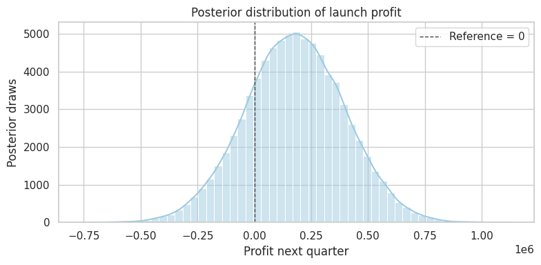
This is where Bayesian analysis often feels very natural for business settings. Instead of translating p-values into decisions indirectly, we simulate the business outcome implied by the posterior causal effect.
The launch decision can still depend on risk tolerance, reversibility, strategic value, and fairness constraints. Bayesian expected value is an input to decision-making, not the entire decision.
12. Bayesian Causal Workflow
A practical Bayesian causal workflow:
workflow = pd.DataFrame(
    [
        {
            "step": "Define causal estimand",
            "question": "ATE, ATT, CATE, policy value, cumulative impact, or decision utility?",
            "artifact": "Estimand statement.",
        },
        {
            "step": "Justify identification",
            "question": "Why are missing potential outcomes learnable from observed data?",
            "artifact": "Design DAG and assumptions.",
        },
        {
            "step": "Choose likelihood",
            "question": "What outcome model connects observed data to potential outcomes?",
            "artifact": "Model specification.",
        },
        {
            "step": "Choose priors",
            "question": "What prior knowledge, regularization, or skepticism is appropriate?",
            "artifact": "Prior predictive checks and sensitivity grid.",
        },
        {
            "step": "Compute posterior",
            "question": "Can we sample or approximate the posterior reliably?",
            "artifact": "Posterior draws and diagnostics.",
        },
        {
            "step": "Posterior predictive checks",
            "question": "Does the model reproduce relevant features of the data?",
            "artifact": "Predicted vs observed plots.",
        },
        {
            "step": "Causal sensitivity",
            "question": "How do unmeasured confounding, measurement error, or transport assumptions affect the result?",
            "artifact": "Bias prior or sensitivity analysis.",
        },
        {
            "step": "Decision analysis",
            "question": "What action maximizes expected utility under uncertainty?",
            "artifact": "Expected value, downside risk, and decision memo.",
        },
    ]
)

workflow| step | question | artifact | |
|---|---|---|---|
| 0 | Define causal estimand | ATE, ATT, CATE, policy value, cumulative impac... | Estimand statement. |
| 1 | Justify identification | Why are missing potential outcomes learnable f... | Design DAG and assumptions. |
| 2 | Choose likelihood | What outcome model connects observed data to p... | Model specification. |
| 3 | Choose priors | What prior knowledge, regularization, or skept... | Prior predictive checks and sensitivity grid. |
| 4 | Compute posterior | Can we sample or approximate the posterior rel... | Posterior draws and diagnostics. |
| 5 | Posterior predictive checks | Does the model reproduce relevant features of ... | Predicted vs observed plots. |
| 6 | Causal sensitivity | How do unmeasured confounding, measurement err... | Bias prior or sensitivity analysis. |
| 7 | Decision analysis | What action maximizes expected utility under u... | Expected value, downside risk, and decision memo. |
13. Industry Decision Memo Example
Here is a concise Bayesian causal memo.
memo = f'''
### Bayesian Causal Decision Memo

**Decision.** Decide whether to launch a checkout intervention to all eligible users next quarter.

**Design.** The effect estimate comes from a randomized A/B test, so treatment assignment is ignorable by design.

**Estimand.** Average effect on conversion probability among users eligible for next-quarter rollout.

**Posterior result.**

- Posterior mean absolute lift: {lift_draws.mean():.4f}
- 95% credible interval: [{np.quantile(lift_draws, 0.025):.4f}, {np.quantile(lift_draws, 0.975):.4f}]
- Probability lift is positive: {np.mean(lift_draws > 0):.3f}
- Probability lift exceeds 0.5 percentage points: {np.mean(lift_draws > 0.005):.3f}

**Business value.**

- Expected next-quarter profit: ${profit_draws.mean():,.0f}
- Probability profit is positive: {np.mean(profit_draws > 0):.3f}
- 95% posterior interval for profit: [${np.quantile(profit_draws, 0.025):,.0f}, ${np.quantile(profit_draws, 0.975):,.0f}]

**Sensitivity.**

- Results should be rechecked for telemetry changes, heterogeneous effects by device type, and transport to international users.
- If implementation cost rises above the current estimate, rerun the decision calculation.

**Recommendation.**

Launch if the team accepts the posterior downside risk and monitoring is in place for conversion, refund rate, and support contacts.
'''.strip()

display(Markdown(memo))
Bayesian Causal Decision Memo
Decision. Decide whether to launch a checkout intervention to all eligible users next quarter.
Design. The effect estimate comes from a randomized A/B test, so treatment assignment is ignorable by design.
Estimand. Average effect on conversion probability among users eligible for next-quarter rollout.
Posterior result.
- Posterior mean absolute lift: 0.0105
- 95% credible interval: [-0.0021, 0.0229]
- Probability lift is positive: 0.949
- Probability lift exceeds 0.5 percentage points: 0.806
Business value.
- Expected next-quarter profit: $178,249
- Probability profit is positive: 0.794
- 95% posterior interval for profit: [$-252,143, $603,502]
Sensitivity.
- Results should be rechecked for telemetry changes, heterogeneous effects by device type, and transport to international users.
- If implementation cost rises above the current estimate, rerun the decision calculation.
Recommendation.
Launch if the team accepts the posterior downside risk and monitoring is in place for conversion, refund rate, and support contacts.
14. Common Failure Modes
- Treating Bayesian posterior certainty as causal identification.
- Using a flexible model to adjust for the wrong covariates.
- Reporting posterior probabilities without stating the prior.
- Hiding prior sensitivity in small experiments.
- Treating narrow posterior intervals as valid when measurement or assignment is flawed.
- Using hierarchical shrinkage to hide real segment differences.
- Applying causal-impact forecasting when control series are contaminated.
- Optimizing expected value while ignoring downside risk, fairness, or reversibility.
- Confusing posterior predictive accuracy with causal validity.
- Forgetting that decision analysis requires costs, benefits, and constraints outside the statistical model.
15. Exercises
- In the binary A/B test, replace the uniform prior with
Beta(50, 450)for both arms. How much does the posterior lift change? - Change the decision threshold from 0.5 percentage points to 1 percentage point. How does the launch probability change?
- In the continuous experiment, reduce the sample size to 200. Compare unadjusted and regression-adjusted posterior intervals.
- In the confounding simulation, increase the effect of unobserved \(U\) on treatment assignment. How does the adjusted-for-\(X\) posterior move?
- In the hierarchical segment example, double the number of tiny segments. Which estimates shrink most?
- In the causal-impact example, add a post-period shock only to the treated market. Can the model distinguish the shock from treatment?
- Build a decision analysis where the cost of a false launch is asymmetric and much larger than the opportunity cost of waiting.
16. Key Takeaways
- Bayesian causal inference combines causal identification assumptions with posterior uncertainty.
- Randomized experiments make Bayesian treatment-effect estimation especially clean.
- Posterior probabilities are useful for decision-making, but they are conditional on model and prior assumptions.
- Bayesian regression adjustment can improve precision, but it does not solve omitted-variable bias.
- Priors matter most when data are weak or decisions are close.
- Hierarchical models stabilize noisy subgroup effects through partial pooling.
- Bayesian causal-impact models are counterfactual forecasting tools; their causal validity depends on control-series assumptions.
- Decision analysis is one of the strongest practical reasons to use Bayesian causal inference in industry.
References
Brodersen, K. H., Gallusser, F., Koehler, J., Remy, N., & Scott, S. L. (2015). Inferring causal impact using Bayesian structural time-series models. The Annals of Applied Statistics, 9(1), 247-274. https://doi.org/10.1214/14-AOAS788
Gelman, A., Carlin, J. B., Stern, H. S., Dunson, D. B., Vehtari, A., & Rubin, D. B. (2013). Bayesian data analysis (3rd ed.). Chapman & Hall/CRC. https://doi.org/10.1201/b16018
Hahn, P. R., Murray, J. S., & Carvalho, C. M. (2020). Bayesian regression tree models for causal inference: Regularization, confounding, and heterogeneous effects. Bayesian Analysis, 15(3), 965-1056. https://doi.org/10.1214/19-BA1195
Hill, J. L. (2011). Bayesian nonparametric modeling for causal inference. Journal of Computational and Graphical Statistics, 20(1), 217-240. https://doi.org/10.1198/jcgs.2010.08162
Imbens, G. W., & Rubin, D. B. (2015). Causal inference for statistics, social, and biomedical sciences: An introduction. Cambridge University Press. https://doi.org/10.1017/CBO9781139025751
Rubin, D. B. (1978). Bayesian inference for causal effects: The role of randomization. The Annals of Statistics, 6(1), 34-58. https://doi.org/10.1214/aos/1176344064