import warnings
warnings.filterwarnings("ignore")

from graphviz import Digraph
from IPython.display import Markdown, display
import matplotlib.pyplot as plt
import numpy as np
import pandas as pd
import seaborn as sns
import statsmodels.formula.api as smf
from scipy.special import expit

sns.set_theme(style="whitegrid", context="notebook")
pd.set_option("display.max_columns", 90)
pd.set_option("display.float_format", lambda x: f"{x:,.3f}")


def regression_effect(model, term):
    estimate = model.params[term]
    se = model.bse[term]
    return pd.Series(
        {
            "estimate": estimate,
            "std_error": se,
            "ci_lower": estimate - 1.96 * se,
            "ci_upper": estimate + 1.96 * se,
            "p_value": model.pvalues[term],
        }
    )


def mean_difference(df, outcome, treatment):
    treated = df.loc[df[treatment] == 1, outcome]
    control = df.loc[df[treatment] == 0, outcome]
    estimate = treated.mean() - control.mean()
    se = np.sqrt(treated.var(ddof=1) / treated.size + control.var(ddof=1) / control.size)
    return pd.Series(
        {
            "estimate": estimate,
            "std_error": se,
            "ci_lower": estimate - 1.96 * se,
            "ci_upper": estimate + 1.96 * se,
            "p_value": np.nan,
        }
    )


def plot_coef_table(table, title, xlabel, reference=0, figsize=(8.5, 4.5)):
    plot_df = table.sort_values("estimate")
    fig, ax = plt.subplots(figsize=figsize)
    ax.errorbar(
        x=plot_df["estimate"],
        y=plot_df.index,
        xerr=[
            plot_df["estimate"] - plot_df["ci_lower"],
            plot_df["ci_upper"] - plot_df["estimate"],
        ],
        fmt="o",
        color="#2b8cbe",
        ecolor="#a6bddb",
        elinewidth=3,
        capsize=4,
    )
    ax.axvline(reference, color="#444444", linestyle="--", linewidth=1)
    ax.set_title(title)
    ax.set_xlabel(xlabel)
    ax.set_ylabel("")
    plt.tight_layout()
return fig, ax04. Measurement Error
Measurement error is one of the quietest ways for a causal analysis to go wrong.
The data may contain exactly the rows we want. The treatment may look well-defined. The adjustment set may look defensible. But if key variables are measured badly, the analysis can estimate the wrong effect.
This notebook treats measurement as part of the causal design. We will separate four cases:
- The outcome is noisy.
- The treatment or exposure is misclassified.
- A confounder is measured with error.
- A proxy is used for a latent construct.
Each case has a different causal consequence. A noisy outcome is not the same problem as a noisy confounder. A noisy treatment is not the same problem as a noisy baseline covariate. A good analyst has to locate the measurement error before choosing a remedy.
Learning Goals
By the end of this notebook, you should be able to:
- Distinguish measurement error in outcomes, treatments, confounders, and mediators.
- Explain why mean-zero outcome noise often reduces precision, while confounder noise can bias causal estimates.
- Use causal diagrams to represent true variables and measured proxies.
- Simulate attenuation from classical measurement error.
- Correct binary treatment misclassification when sensitivity and specificity are known or estimated from validation data.
- Use validation data, replicate measures, and SIMEX-style sensitivity analysis to reason about noisy confounders.
- Write an industry measurement-error plan for a causal project.
1. Setup
We will use the same core stack as the previous notebooks: pandas, numpy, statsmodels, seaborn, matplotlib, and Graphviz.
2. Measurement Error as a Causal Object
Let \(X\) denote the true variable and \(X^\ast\) denote the measured variable.
A simple classical measurement-error model is:
\[ X^\ast = X + U \]
where:
\[ E[U \mid X, A, Y] = 0 \]
This looks harmless, but its causal effect depends on what \(X\) is.
- If \(X\) is the outcome and the error is mean-zero, the treatment effect on the mean outcome can remain unbiased, but noisier.
- If \(X\) is the treatment, treatment groups are mixed together.
- If \(X\) is a confounder, adjustment is incomplete because \(X^\ast\) does not fully block the backdoor path.
- If \(X\) is a mediator or post-treatment variable, measurement error can distort decomposition or mechanism claims.
dot = Digraph("measurement_error_dag", graph_attr={"rankdir": "LR"})
dot.attr("node", shape="box", style="rounded,filled", fillcolor="#f7fbff", color="#6baed6")

dot.node("X", "True confounder X")
dot.node("A", "Treatment A")
dot.node("Y", "Outcome Y")
dot.node("Xstar", "Measured proxy X*")
dot.node("U", "Measurement noise U", fillcolor="#fee0d2", color="#fc9272")

dot.edge("X", "A")
dot.edge("X", "Y")
dot.edge("A", "Y")
dot.edge("X", "Xstar")
dot.edge("U", "Xstar")

dot
The diagram shows a core causal problem: if \(X\) confounds \(A \rightarrow Y\), adjusting for \(X^\ast\) is not the same as adjusting for \(X\).
Kuroki and Pearl (2014) study this kind of measurement-bias problem using causal diagrams and discuss conditions under which proxy variables and external information can restore causal effects.
3. A Taxonomy for Causal Work
Before choosing a method, classify the measurement problem.
measurement_taxonomy = pd.DataFrame(
    [
        {
            "measured_variable": "Outcome Y",
            "example": "Revenue from an unreliable event pipeline",
            "typical_effect": "Mean-zero noise inflates variance; systematic or differential error biases effects.",
            "common_response": "Audit outcome definition; improve instrumentation; sensitivity analysis.",
        },
        {
            "measured_variable": "Treatment A",
            "example": "CRM says a customer received outreach, but logs disagree",
            "typical_effect": "Groups are mixed; effects are often attenuated or can change direction.",
            "common_response": "Use assignment logs; validation sample; misclassification correction.",
        },
        {
            "measured_variable": "Confounder X",
            "example": "Customer intent measured by a noisy score",
            "typical_effect": "Residual confounding remains after adjustment.",
            "common_response": "Collect better proxies; validation data; replicate measures; sensitivity analysis.",
        },
        {
            "measured_variable": "Mediator M",
            "example": "Engagement score used to explain why treatment worked",
            "typical_effect": "Direct/indirect effect decomposition becomes fragile.",
            "common_response": "Pre-specify measurement model; avoid overclaiming mechanisms.",
        },
    ]
)

measurement_taxonomy| measured_variable | example | typical_effect | common_response | |
|---|---|---|---|---|
| 0 | Outcome Y | Revenue from an unreliable event pipeline | Mean-zero noise inflates variance; systematic ... | Audit outcome definition; improve instrumentat... |
| 1 | Treatment A | CRM says a customer received outreach, but log... | Groups are mixed; effects are often attenuated... | Use assignment logs; validation sample; miscla... |
| 2 | Confounder X | Customer intent measured by a noisy score | Residual confounding remains after adjustment. | Collect better proxies; validation data; repli... |
| 3 | Mediator M | Engagement score used to explain why treatment... | Direct/indirect effect decomposition becomes f... | Pre-specify measurement model; avoid overclaim... |
4. Simulation 1: Noisy Outcomes in a Randomized Experiment
Start with the cleanest setting: randomized treatment and a continuous outcome.
The true data-generating process is:
\[ Y = \alpha + \tau A + \epsilon \]
where \(A\) is randomized. Now suppose the measured outcome is:
\[ Y^\ast = Y + U \]
If \(E[U \mid A] = 0\), the difference in mean observed outcomes still targets \(\tau\). If \(E[U \mid A] \neq 0\), the measured outcome contains treatment-related measurement bias.
rng = np.random.default_rng(4204)
n = 6000
true_tau = 2.0

df_outcome = pd.DataFrame(
    {
        "A": rng.binomial(1, 0.5, size=n),
        "baseline": rng.normal(0, 1, size=n),
    }
)

df_outcome["Y_true"] = (
    10
    + true_tau * df_outcome["A"]
    + 0.8 * df_outcome["baseline"]
    + rng.normal(0, 2.0, size=n)
)

df_outcome["Y_meanzero_noise"] = df_outcome["Y_true"] + rng.normal(0, 4.0, size=n)
df_outcome["Y_treatment_related_noise"] = (
    df_outcome["Y_true"]
    + rng.normal(0, 4.0, size=n)
    + 1.1 * df_outcome["A"]
)

outcome_estimates = pd.DataFrame(
    {
        "True outcome": mean_difference(df_outcome, "Y_true", "A"),
        "Mean-zero noisy outcome": mean_difference(df_outcome, "Y_meanzero_noise", "A"),
        "Treatment-related measurement bias": mean_difference(df_outcome, "Y_treatment_related_noise", "A"),
    }
).T

outcome_estimates| estimate | std_error | ci_lower | ci_upper | p_value | |
|---|---|---|---|---|---|
| True outcome | 1.938 | 0.056 | 1.828 | 2.049 | NaN |
| Mean-zero noisy outcome | 2.002 | 0.118 | 1.771 | 2.233 | NaN |
| Treatment-related measurement bias | 2.961 | 0.116 | 2.733 | 3.189 | NaN |
plot_coef_table(
    outcome_estimates,
    title="Noisy outcomes are not all the same problem",
    xlabel="Estimated treatment effect",
    reference=true_tau,
    figsize=(8, 3.8),
)
plt.show()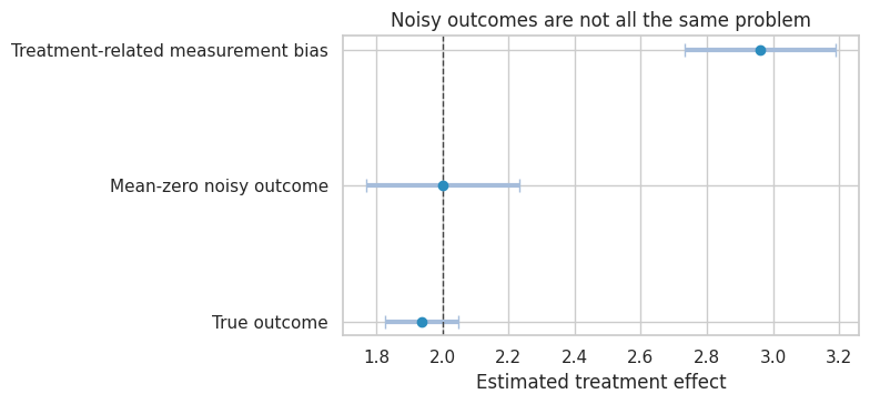
Interpretation
The mean-zero noisy outcome remains centered near the true effect, but the interval is wider because the outcome has more variance.
The treatment-related measurement error moves the estimate. This is not a precision problem. It is a validity problem. In industry settings, this can happen when treatment affects tracking itself:
- A new checkout flow changes what events are fired.
- A sales outreach program changes how account managers enter notes.
- A model intervention changes the probability that users opt into telemetry.
The right response is not simply “collect more rows.” More rows can make the biased estimate more precise.
5. Simulation 2: Treatment Misclassification
Now suppose the outcome is measured correctly, but treatment receipt is misclassified.
Let \(A\) be true treatment and \(A^\ast\) be recorded treatment. For a binary treatment:
\[ Sensitivity = P(A^\ast = 1 \mid A = 1) \]
\[ Specificity = P(A^\ast = 0 \mid A = 0) \]
If sensitivity and specificity are imperfect, the observed treated and control groups are mixtures of the true groups.
rng = np.random.default_rng(4205)
n = 7000
tau_treatment = 3.0
sens_A = 0.86
spec_A = 0.91

df_treat = pd.DataFrame({"A_true": rng.binomial(1, 0.48, size=n)})
df_treat["Y"] = 25 + tau_treatment * df_treat["A_true"] + rng.normal(0, 5, size=n)

observed_when_true_treated = rng.binomial(1, sens_A, size=n)
false_positive_when_true_control = rng.binomial(1, 1 - spec_A, size=n)
df_treat["A_observed"] = np.where(
    df_treat["A_true"] == 1,
    observed_when_true_treated,
    false_positive_when_true_control,
)

treatment_misclass_estimates = pd.DataFrame(
    {
        "Oracle: true treatment": mean_difference(df_treat, "Y", "A_true"),
        "Naive: recorded treatment": mean_difference(df_treat, "Y", "A_observed"),
    }
).T

treatment_misclass_estimates| estimate | std_error | ci_lower | ci_upper | p_value | |
|---|---|---|---|---|---|
| Oracle: true treatment | 3.093 | 0.120 | 2.858 | 3.328 | NaN |
| Naive: recorded treatment | 2.389 | 0.123 | 2.148 | 2.629 | NaN |
confusion = pd.crosstab(
    df_treat["A_true"],
    df_treat["A_observed"],
    normalize="index",
).rename_axis(index="True treatment", columns="Recorded treatment")

confusion| Recorded treatment | 0 | 1 |
|---|---|---|
| True treatment | ||
| 0 | 0.908 | 0.092 |
| 1 | 0.148 | 0.852 |
The naive estimate is smaller because the recorded treatment groups contain contamination:
- Some truly treated units appear in the recorded-control group.
- Some truly untreated units appear in the recorded-treated group.
This is the treatment analogue of a blurred camera. The contrast between groups gets softened.
Matrix Correction When Sensitivity and Specificity Are Known
If misclassification is independent of the outcome conditional on true treatment, we can express observed counts and observed outcome sums as mixtures of true counts and true outcome sums.
Let:
\[ Q = \begin{bmatrix} P(A^\ast=0 \mid A=0) & P(A^\ast=0 \mid A=1) \\ P(A^\ast=1 \mid A=0) & P(A^\ast=1 \mid A=1) \end{bmatrix} = \begin{bmatrix} specificity & 1 - sensitivity \\ 1 - specificity & sensitivity \end{bmatrix} \]
Then:
\[ \begin{bmatrix} N^\ast_0 \\ N^\ast_1 \end{bmatrix} = Q \begin{bmatrix} N_0 \\ N_1 \end{bmatrix} \]
and the same mixing applies to outcome sums.
def correct_binary_treatment_misclassification(df, observed_treatment, outcome, sensitivity, specificity):
    q = np.array(
        [
            [specificity, 1 - sensitivity],
            [1 - specificity, sensitivity],
        ]
    )
    counts_observed = (
        df.groupby(observed_treatment)
        .size()
        .reindex([0, 1], fill_value=0)
        .to_numpy(dtype=float)
    )
    sums_observed = (
        df.groupby(observed_treatment)[outcome]
        .sum()
        .reindex([0, 1], fill_value=0)
        .to_numpy(dtype=float)
    )

    counts_true_hat = np.linalg.solve(q, counts_observed)
    sums_true_hat = np.linalg.solve(q, sums_observed)
    means_true_hat = sums_true_hat / counts_true_hat
    return means_true_hat[1] - means_true_hat[0]


corrected_known = correct_binary_treatment_misclassification(
    df_treat,
    observed_treatment="A_observed",
    outcome="Y",
    sensitivity=sens_A,
    specificity=spec_A,
)

treatment_misclass_estimates.loc["Corrected: known sensitivity/specificity"] = {
    "estimate": corrected_known,
    "std_error": np.nan,
    "ci_lower": np.nan,
    "ci_upper": np.nan,
    "p_value": np.nan,
}

treatment_misclass_estimates| estimate | std_error | ci_lower | ci_upper | p_value | |
|---|---|---|---|---|---|
| Oracle: true treatment | 3.093 | 0.120 | 2.858 | 3.328 | NaN |
| Naive: recorded treatment | 2.389 | 0.123 | 2.148 | 2.629 | NaN |
| Corrected: known sensitivity/specificity | 3.088 | NaN | NaN | NaN | NaN |
fig, ax = plt.subplots(figsize=(8, 3.8))
display_df = treatment_misclass_estimates.reset_index(names="method")
sns.pointplot(data=display_df, y="method", x="estimate", join=False, ax=ax, color="#2b8cbe")
ax.axvline(tau_treatment, color="#444444", linestyle="--", linewidth=1, label="True effect")
ax.set_title("Treatment misclassification attenuates the treatment contrast")
ax.set_xlabel("Estimated treatment effect")
ax.set_ylabel("")
ax.legend()
plt.tight_layout()
plt.show()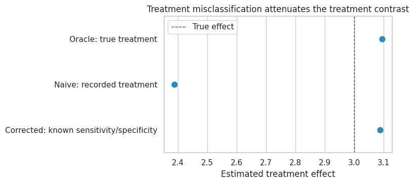
Validation Data
In practice, we rarely know sensitivity and specificity exactly. We estimate them from a validation sample where the true treatment status is audited.
This validation sample might come from:
- manual CRM review,
- raw exposure logs,
- product instrumentation audit,
- medical chart review,
- customer-support transcript review.
validation = df_treat.sample(800, random_state=17)

sens_hat = validation.loc[validation["A_true"] == 1, "A_observed"].mean()
spec_hat = 1 - validation.loc[validation["A_true"] == 0, "A_observed"].mean()

corrected_validation = correct_binary_treatment_misclassification(
    df_treat,
    observed_treatment="A_observed",
    outcome="Y",
    sensitivity=sens_hat,
    specificity=spec_hat,
)

validation_summary = pd.DataFrame(
    {
        "quantity": ["Sensitivity", "Specificity", "Corrected effect"],
        "true_or_oracle": [sens_A, spec_A, tau_treatment],
        "estimated_from_validation": [sens_hat, spec_hat, corrected_validation],
    }
)

validation_summary| quantity | true_or_oracle | estimated_from_validation | |
|---|---|---|---|
| 0 | Sensitivity | 0.860 | 0.856 |
| 1 | Specificity | 0.910 | 0.907 |
| 2 | Corrected effect | 3.000 | 3.117 |
The correction is only as credible as the validation design. If the validation sample overrepresents clean cases, active users, high-value customers, or recent records, its sensitivity and specificity may not represent the full analysis population.
6. Simulation 3: Noisy Confounders
Confounder measurement error is often more dangerous than outcome noise.
Suppose:
\[ X \rightarrow A \]
and:
\[ X \rightarrow Y \]
If we observe only \(X^\ast\), adjustment for \(X^\ast\) leaves residual confounding because units with the same measured score still differ in true \(X\).
rng = np.random.default_rng(4206)
n = 9000
true_tau_conf = 1.5

df_conf = pd.DataFrame({"X_true": rng.normal(0, 1, size=n)})
df_conf["A"] = rng.binomial(1, expit(-0.15 + 1.25 * df_conf["X_true"]), size=n)
df_conf["Y"] = (
    5
    + true_tau_conf * df_conf["A"]
    + 2.2 * df_conf["X_true"]
    + rng.normal(0, 1.5, size=n)
)

sigma_measure = 1.15
df_conf["X_claims_proxy"] = df_conf["X_true"] + rng.normal(0, sigma_measure, size=n)
df_conf["X_survey_proxy"] = df_conf["X_true"] + rng.normal(0, sigma_measure, size=n)
df_conf["X_proxy_average"] = (df_conf["X_claims_proxy"] + df_conf["X_survey_proxy"]) / 2

models_conf = {
    "Unadjusted": smf.ols("Y ~ A", data=df_conf).fit(),
    "Adjust for one noisy proxy": smf.ols("Y ~ A + X_claims_proxy", data=df_conf).fit(),
    "Adjust for two-proxy average": smf.ols("Y ~ A + X_proxy_average", data=df_conf).fit(),
    "Oracle: adjust for true X": smf.ols("Y ~ A + X_true", data=df_conf).fit(),
}

confounder_error_results = pd.DataFrame(
    {name: regression_effect(model, "A") for name, model in models_conf.items()}
).T

confounder_error_results| estimate | std_error | ci_lower | ci_upper | p_value | |
|---|---|---|---|---|---|
| Unadjusted | 3.664 | 0.052 | 3.563 | 3.766 | 0.000 |
| Adjust for one noisy proxy | 2.838 | 0.047 | 2.745 | 2.931 | 0.000 |
| Adjust for two-proxy average | 2.471 | 0.045 | 2.383 | 2.560 | 0.000 |
| Oracle: adjust for true X | 1.487 | 0.036 | 1.416 | 1.557 | 0.000 |
plot_coef_table(
    confounder_error_results,
    title="Noisy confounders leave residual confounding",
    xlabel="Coefficient on treatment",
    reference=true_tau_conf,
    figsize=(8, 4.2),
)
plt.show()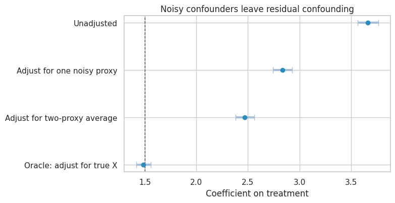
Interpretation
The unadjusted estimate is biased because high-\(X\) units are more likely to receive treatment and also have higher outcomes.
Adjusting for one noisy proxy helps but does not fully remove confounding. Averaging two independent proxies improves adjustment because the average is closer to the true latent confounder. The oracle model shows the estimate we would get if the true confounder were measured.
This is a common industry pattern:
- “Customer intent” is measured by recent clicks.
- “Account health” is measured by a risk score.
- “Disease severity” is measured by claims codes.
- “Manager quality” is measured by lagged team metrics.
These proxies can be useful, but they should not be mistaken for the construct itself.
7. Reliability Ratio and Attenuation
In a simple linear errors-in-variables problem:
\[ X^\ast = X + U \]
with \(U\) independent of \(X\), the reliability ratio is:
\[ \lambda = \frac{Var(X)}{Var(X) + Var(U)} \]
In a simple regression of \(Y\) on \(X^\ast\), the slope is attenuated toward zero by approximately \(\lambda\).
In causal adjustment, the same intuition helps: lower reliability means less confounding is removed.
reliability_table = []
for sigma in [0.25, 0.5, 1.0, 1.5, 2.0]:
    tmp = df_conf.copy()
    tmp["X_star"] = tmp["X_true"] + rng.normal(0, sigma, size=tmp.shape[0])
    model = smf.ols("Y ~ A + X_star", data=tmp).fit()
    reliability = tmp["X_true"].var() / tmp["X_star"].var()
    reliability_table.append(
        {
            "measurement_sd": sigma,
            "empirical_reliability": reliability,
            "treatment_estimate": model.params["A"],
            "absolute_bias": abs(model.params["A"] - true_tau_conf),
        }
    )

reliability_table = pd.DataFrame(reliability_table)
reliability_table| measurement_sd | empirical_reliability | treatment_estimate | absolute_bias | |
|---|---|---|---|---|
| 0 | 0.250 | 0.941 | 1.638 | 0.138 |
| 1 | 0.500 | 0.791 | 2.038 | 0.538 |
| 2 | 1.000 | 0.501 | 2.716 | 1.216 |
| 3 | 1.500 | 0.321 | 3.118 | 1.618 |
| 4 | 2.000 | 0.202 | 3.292 | 1.792 |
fig, axes = plt.subplots(1, 2, figsize=(12, 4))

sns.lineplot(
    data=reliability_table,
    x="measurement_sd",
    y="empirical_reliability",
    marker="o",
    ax=axes[0],
)
axes[0].set_title("More measurement noise lowers reliability")
axes[0].set_xlabel("Measurement-error SD")
axes[0].set_ylabel("Reliability ratio")

sns.lineplot(
    data=reliability_table,
    x="measurement_sd",
    y="treatment_estimate",
    marker="o",
    ax=axes[1],
)
axes[1].axhline(true_tau_conf, color="#444444", linestyle="--", linewidth=1)
axes[1].set_title("Less reliable confounders remove less bias")
axes[1].set_xlabel("Measurement-error SD")
axes[1].set_ylabel("Treatment estimate")

plt.tight_layout()
plt.show()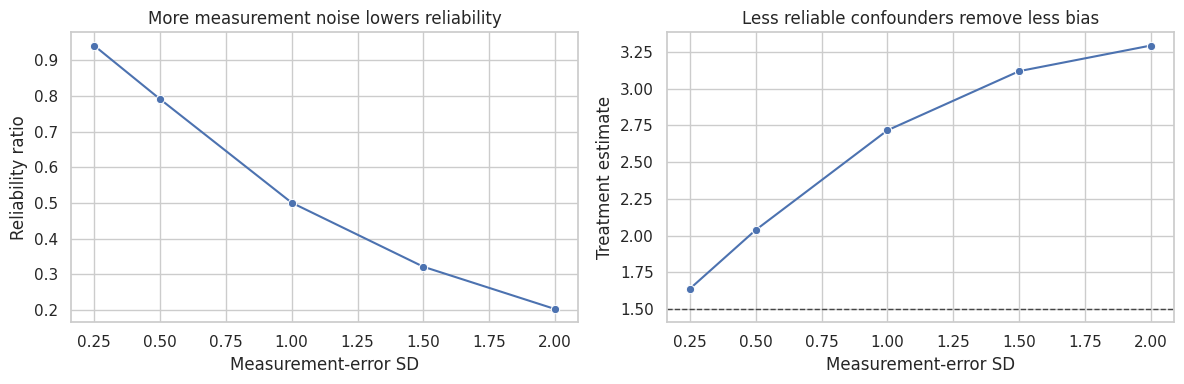
The right diagnostic is not only whether a proxy is predictive. It is whether it is reliable enough to block confounding paths for the causal question.
8. Validation Data and Calibration
Validation data means that for some units we observe both:
\[ X^\ast \]
and:
\[ X \]
That lets us learn how the proxy relates to the truth. Validation data can be internal or external:
- internal audit sample,
- duplicate survey,
- chart review,
- lab validation,
- high-quality data vendor sample,
- historical period with both old and new measurement systems.
Here we fit a calibration model for the true confounder using two proxies in a validation subset.
validation_conf = df_conf.sample(900, random_state=31).copy()

calibration_model = smf.ols(
    "X_true ~ X_claims_proxy + X_survey_proxy",
    data=validation_conf,
).fit()

df_conf["X_calibrated"] = calibration_model.predict(df_conf)

calibrated_model = smf.ols("Y ~ A + X_calibrated", data=df_conf).fit()
both_proxy_model = smf.ols("Y ~ A + X_claims_proxy + X_survey_proxy", data=df_conf).fit()

validation_results = confounder_error_results.copy()
validation_results.loc["Validation-calibrated proxy"] = regression_effect(calibrated_model, "A")
validation_results.loc["Adjust for both proxies directly"] = regression_effect(both_proxy_model, "A")

validation_results| estimate | std_error | ci_lower | ci_upper | p_value | |
|---|---|---|---|---|---|
| Unadjusted | 3.664 | 0.052 | 3.563 | 3.766 | 0.000 |
| Adjust for one noisy proxy | 2.838 | 0.047 | 2.745 | 2.931 | 0.000 |
| Adjust for two-proxy average | 2.471 | 0.045 | 2.383 | 2.560 | 0.000 |
| Oracle: adjust for true X | 1.487 | 0.036 | 1.416 | 1.557 | 0.000 |
| Validation-calibrated proxy | 2.472 | 0.045 | 2.383 | 2.561 | 0.000 |
| Adjust for both proxies directly | 2.472 | 0.045 | 2.383 | 2.560 | 0.000 |
plot_coef_table(
    validation_results,
    title="Validation and multiple proxies move the estimate toward the oracle",
    xlabel="Coefficient on treatment",
    reference=true_tau_conf,
    figsize=(8.5, 4.8),
)
plt.show()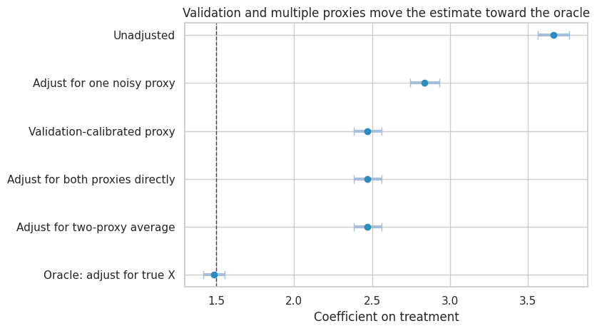
Practical Warning
In this linear example, calibration and direct proxy adjustment are close because the calibration model is a linear combination of observed proxies. In more complex settings, validation data can support:
- nonlinear calibration,
- multiple imputation of the true confounder,
- likelihood-based measurement-error models,
- Bayesian measurement models,
- sensitivity analysis over plausible reliability levels.
The deeper point is not that one calibration recipe always solves the problem. The point is that validation information changes measurement error from an invisible assumption into an estimable design component.
9. SIMEX-Style Sensitivity Analysis
SIMEX stands for simulation-extrapolation. The idea is:
- Add extra measurement error to the already noisy covariate.
- Estimate the causal model at several extra-noise levels.
- Extrapolate the trend back to a hypothetical no-error setting.
This is not magic. It depends on assumptions about the error process. But it is useful as a transparent sensitivity analysis.
rng = np.random.default_rng(4207)
lambda_grid = np.array([0.0, 0.5, 1.0, 1.5, 2.0])
rows = []

for lam in lambda_grid:
    for rep in range(60):
        extra_noise = rng.normal(0, np.sqrt(lam) * sigma_measure, size=df_conf.shape[0])
        tmp = df_conf.assign(X_simex=df_conf["X_claims_proxy"] + extra_noise)
        est = smf.ols("Y ~ A + X_simex", data=tmp).fit().params["A"]
        rows.append({"lambda": lam, "rep": rep, "estimate": est})

simex_df = pd.DataFrame(rows)
simex_mean = simex_df.groupby("lambda", as_index=False)["estimate"].mean()

quadratic = np.polyfit(simex_mean["lambda"], simex_mean["estimate"], deg=2)
simex_extrapolated = np.polyval(quadratic, -1)

simex_summary = pd.DataFrame(
    {
        "method": [
            "Naive noisy-confounder adjustment",
            "SIMEX extrapolation to lambda = -1",
            "Oracle true-confounder adjustment",
        ],
        "estimate": [
            confounder_error_results.loc["Adjust for one noisy proxy", "estimate"],
            simex_extrapolated,
            confounder_error_results.loc["Oracle: adjust for true X", "estimate"],
        ],
    }
)

simex_mean, simex_summary
( lambda estimate
0 0.000 2.838
1 0.500 3.034
2 1.000 3.152
3 1.500 3.239
4 2.000 3.298,
method estimate
0 Naive noisy-confounder adjustment 2.838
1 SIMEX extrapolation to lambda = -1 2.356
2 Oracle true-confounder adjustment 1.487)lambda_plot = np.linspace(-1, 2.2, 100)
pred_plot = np.polyval(quadratic, lambda_plot)
fig, ax = plt.subplots(figsize=(8, 4.5))
sns.scatterplot(data=simex_df, x="lambda", y="estimate", alpha=0.12, ax=ax, color="#9ecae1")
sns.lineplot(data=simex_mean, x="lambda", y="estimate", marker="o", ax=ax, color="#08519c", label="Mean estimate")
ax.plot(lambda_plot, pred_plot, color="#de2d26", label="Quadratic extrapolation")
ax.axvline(-1, color="#444444", linestyle="--", linewidth=1, label="No-error target")
ax.axhline(true_tau_conf, color="#31a354", linestyle=":", linewidth=2, label="True effect")
ax.set_title("SIMEX: add noise, observe bias trend, extrapolate backward")
ax.set_xlabel("Extra measurement-error multiplier")
ax.set_ylabel("Treatment estimate")
ax.legend()
plt.tight_layout()
plt.show()
simex_summary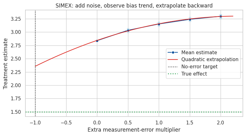
| method | estimate | |
|---|---|---|
| 0 | Naive noisy-confounder adjustment | 2.838 |
| 1 | SIMEX extrapolation to lambda = -1 | 2.356 |
| 2 | Oracle true-confounder adjustment | 1.487 |
Interpretation
As extra noise is added to the confounder, the adjusted estimate drifts toward the unadjusted confounded estimate. Extrapolating backward gives a rough estimate of what might happen if the measurement error were removed.
This is best used as a sensitivity analysis, not as a replacement for good measurement.
10. Binary Outcome Misclassification
Continuous measurement error is not the only problem. Binary outcomes and binary labels can also be misclassified.
For a binary outcome:
\[ Y^\ast \in \{0,1\} \]
with sensitivity and specificity:
\[ P(Y^\ast=1 \mid Y=1) = Se \]
\[ P(Y^\ast=0 \mid Y=0) = Sp \]
If \(Se + Sp > 1\), an observed risk can be corrected by:
\[ \widehat{P}(Y=1) = \frac{\widehat{P}(Y^\ast=1) + Sp - 1}{Se + Sp - 1} \]
rng = np.random.default_rng(4208)
n = 8000
df_binary = pd.DataFrame({"A": rng.binomial(1, 0.5, size=n)})

p0 = 0.18
risk_difference_true = 0.08
df_binary["p_true"] = p0 + risk_difference_true * df_binary["A"]
df_binary["Y_true"] = rng.binomial(1, df_binary["p_true"])

sens_y = 0.82
spec_y = 0.93
draw = rng.uniform(size=n)
df_binary["Y_observed"] = np.where(
    df_binary["Y_true"] == 1,
    (draw < sens_y).astype(int),
    (draw > spec_y).astype(int),
)

def risk_difference(df, outcome):
    return (
        df.loc[df["A"] == 1, outcome].mean()
        - df.loc[df["A"] == 0, outcome].mean()
    )


def correct_binary_risk(p_observed, sensitivity, specificity):
    return (p_observed + specificity - 1) / (sensitivity + specificity - 1)


observed_risks = df_binary.groupby("A")["Y_observed"].mean()
corrected_risks = observed_risks.apply(
    lambda p: correct_binary_risk(p, sens_y, spec_y)
)

binary_misclass_results = pd.DataFrame(
    {
        "method": [
            "Oracle: true outcome",
            "Naive: misclassified outcome",
            "Corrected with known Se/Sp",
        ],
        "risk_difference": [
            risk_difference(df_binary, "Y_true"),
            risk_difference(df_binary, "Y_observed"),
            corrected_risks.loc[1] - corrected_risks.loc[0],
        ],
    }
)

binary_misclass_results| method | risk_difference | |
|---|---|---|
| 0 | Oracle: true outcome | 0.082 |
| 1 | Naive: misclassified outcome | 0.059 |
| 2 | Corrected with known Se/Sp | 0.079 |
fig, ax = plt.subplots(figsize=(8, 3.8))
sns.pointplot(data=binary_misclass_results, y="method", x="risk_difference", join=False, ax=ax, color="#2b8cbe")
ax.axvline(risk_difference_true, color="#444444", linestyle="--", linewidth=1, label="True risk difference")
ax.set_title("Outcome misclassification can attenuate risk differences")
ax.set_xlabel("Risk difference")
ax.set_ylabel("")
ax.legend()
plt.tight_layout()
plt.show()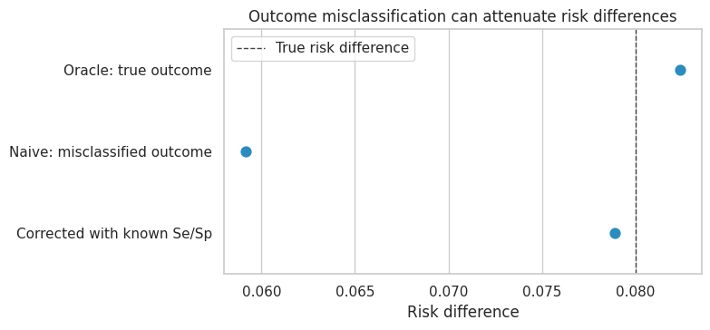
Why This Matters for Industry
Binary outcomes are everywhere:
- churned or not,
- converted or not,
- fraud or not,
- retained or not,
- escalated support ticket or not.
The label is often a measurement process. If fraud labels depend on manual investigation, then the measured label reflects both fraud and investigation intensity. If churn labels depend on delayed billing data, the measured label reflects true churn and data latency.
11. Probabilistic Bias Analysis
Quantitative bias analysis makes measurement assumptions explicit. Instead of pretending sensitivity and specificity are known, assign plausible distributions and propagate them through the correction.
Lash, Fox, and Fink (2009) provide a broad epidemiologic treatment of quantitative bias analysis. The same idea is useful in business and platform settings.
rng = np.random.default_rng(4209)
bias_draws = 4000

sens_draw = rng.beta(82, 18, size=bias_draws)
spec_draw = rng.beta(93, 7, size=bias_draws)

p_obs_control = observed_risks.loc[0]
p_obs_treated = observed_risks.loc[1]

corrected_control = correct_binary_risk(p_obs_control, sens_draw, spec_draw)
corrected_treated = correct_binary_risk(p_obs_treated, sens_draw, spec_draw)
corrected_rd = corrected_treated - corrected_control

bias_analysis_summary = pd.Series(
    {
        "naive_observed_rd": risk_difference(df_binary, "Y_observed"),
        "median_corrected_rd": np.median(corrected_rd),
        "p05_corrected_rd": np.quantile(corrected_rd, 0.05),
        "p95_corrected_rd": np.quantile(corrected_rd, 0.95),
        "oracle_true_rd": risk_difference(df_binary, "Y_true"),
    }
)

bias_analysis_summary
naive_observed_rd 0.059
median_corrected_rd 0.079
p05_corrected_rd 0.072
p95_corrected_rd 0.088
oracle_true_rd 0.082
dtype: float64fig, ax = plt.subplots(figsize=(8, 4))
sns.histplot(corrected_rd, bins=45, kde=True, color="#9ecae1", ax=ax)
ax.axvline(risk_difference(df_binary, "Y_observed"), color="#de2d26", linestyle="--", label="Naive observed")
ax.axvline(risk_difference_true, color="#31a354", linestyle=":", linewidth=2, label="True RD")
ax.set_title("Probabilistic bias analysis for outcome misclassification")
ax.set_xlabel("Corrected risk difference")
ax.set_ylabel("Simulation count")
ax.legend()
plt.tight_layout()
plt.show()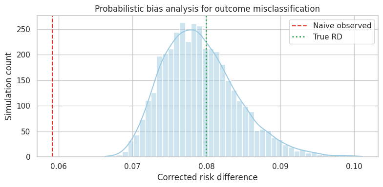
The result is no longer a single corrected estimate. It is a distribution over corrected estimates induced by uncertainty in measurement quality.
This is often the honest format for decision-making. It separates:
- random sampling uncertainty,
- uncertainty about the causal design,
- uncertainty about measurement validity.
12. Measurement Error in Mediators
Measurement error in mediators is especially easy to overinterpret.
Suppose:
\[ A \rightarrow M \rightarrow Y \]
and we observe:
\[ M^\ast = M + U \]
If we estimate mediation effects using \(M^\ast\), the indirect effect can be attenuated, distorted, or made to look absent even when the underlying mechanism is strong.
dot = Digraph("mediator_measurement", graph_attr={"rankdir": "LR"})
dot.attr("node", shape="box", style="rounded,filled", fillcolor="#f7fbff", color="#6baed6")

dot.node("A", "Treatment A")
dot.node("M", "True mediator M")
dot.node("Y", "Outcome Y")
dot.node("Mstar", "Measured mediator M*")
dot.node("U", "Measurement noise U", fillcolor="#fee0d2", color="#fc9272")

dot.edge("A", "M")
dot.edge("M", "Y")
dot.edge("A", "Y")
dot.edge("M", "Mstar")
dot.edge("U", "Mstar")

dot
A useful professional habit is to downgrade mechanism claims when mediator measurement is weak.
It may be reasonable to say:
The treatment improved revenue, and engagement increased after treatment.
It is stronger, and often less justified, to say:
The treatment improved revenue because engagement increased.
The second statement requires a mediation design and a credible mediator measurement model.
13. Industry Measurement-Error Checklist
For each important causal variable, ask:
checklist = pd.DataFrame(
    [
        {
            "question": "What is the true construct?",
            "example": "Customer intent, actual exposure, real churn, clinical severity",
        },
        {
            "question": "What is the measured field?",
            "example": "Click count, logged campaign flag, billing cancel flag, claims score",
        },
        {
            "question": "Who or what records it?",
            "example": "Frontend event, backend service, salesperson, manual reviewer",
        },
        {
            "question": "Can treatment affect measurement?",
            "example": "New UI changes event firing; outreach changes CRM entry behavior",
        },
        {
            "question": "Is there validation data?",
            "example": "Audit sample, duplicate source, raw logs, gold-standard panel",
        },
        {
            "question": "Is error likely differential?",
            "example": "Measurement quality differs by treatment, segment, geography, or time",
        },
        {
            "question": "What sensitivity analysis is decision-relevant?",
            "example": "How bad must sensitivity/specificity be to change the launch decision?",
        },
    ]
)

checklist| question | example | |
|---|---|---|
| 0 | What is the true construct? | Customer intent, actual exposure, real churn, ... |
| 1 | What is the measured field? | Click count, logged campaign flag, billing can... |
| 2 | Who or what records it? | Frontend event, backend service, salesperson, ... |
| 3 | Can treatment affect measurement? | New UI changes event firing; outreach changes ... |
| 4 | Is there validation data? | Audit sample, duplicate source, raw logs, gold... |
| 5 | Is error likely differential? | Measurement quality differs by treatment, segm... |
| 6 | What sensitivity analysis is decision-relevant? | How bad must sensitivity/specificity be to cha... |
14. Decision Memo Example
A concise measurement-error memo for an industry causal project might look like this:
memo = '''
### Measurement-Error Memo

**Decision context.** Estimate the effect of a retention intervention on 30-day renewal.

**Main risk.** The renewal outcome is based on billing events. A migration changed event timing during the experiment window, so outcome measurement may differ by treatment cohort.

**Variables at risk.**

- Treatment: assignment is reliable because it comes from experiment allocation logs.
- Outcome: renewal label may be delayed or misclassified.
- Confounders: pre-period customer health score is a proxy, not the construct itself.

**Primary analysis.**

- Use assignment logs for treatment.
- Define renewal from reconciled billing tables rather than frontend events.
- Adjust for pre-treatment health score, contract value, tenure, and product usage.

**Validation plan.**

- Audit a random sample of accounts against finance records.
- Estimate sensitivity and specificity of the renewal label by treatment arm.
- Compare estimates using raw labels, reconciled labels, and bias-corrected labels.

**Sensitivity question.**

- Would the launch decision change if renewal sensitivity differed by 5 percentage points across arms?

**Reporting rule.**

- Report the causal estimate and a measurement-error sensitivity interval, not only the conventional confidence interval.
'''.strip()

display(Markdown(memo))
Measurement-Error Memo
Decision context. Estimate the effect of a retention intervention on 30-day renewal.
Main risk. The renewal outcome is based on billing events. A migration changed event timing during the experiment window, so outcome measurement may differ by treatment cohort.
Variables at risk.
- Treatment: assignment is reliable because it comes from experiment allocation logs.
- Outcome: renewal label may be delayed or misclassified.
- Confounders: pre-period customer health score is a proxy, not the construct itself.
Primary analysis.
- Use assignment logs for treatment.
- Define renewal from reconciled billing tables rather than frontend events.
- Adjust for pre-treatment health score, contract value, tenure, and product usage.
Validation plan.
- Audit a random sample of accounts against finance records.
- Estimate sensitivity and specificity of the renewal label by treatment arm.
- Compare estimates using raw labels, reconciled labels, and bias-corrected labels.
Sensitivity question.
- Would the launch decision change if renewal sensitivity differed by 5 percentage points across arms?
Reporting rule.
- Report the causal estimate and a measurement-error sensitivity interval, not only the conventional confidence interval.
15. Common Failure Modes
- Treating a proxy as the true construct.
- Adjusting for a noisy confounder and declaring confounding solved.
- Ignoring treatment effects on measurement systems.
- Using validation data from an unrepresentative subset.
- Reporting narrow confidence intervals while hiding measurement uncertainty.
- Correcting for misclassification with sensitivity and specificity values that are guesses, without sensitivity analysis.
- Making mechanism claims from noisy mediator measurements.
16. Exercises
- In the noisy outcome simulation, change the treatment-related measurement bias from \(1.1\) to \(-1.1\). What happens to the treatment effect?
- In the treatment misclassification simulation, reduce sensitivity to \(0.70\). How does the naive estimate change?
- In the noisy confounder simulation, increase the measurement-error standard deviation to \(2.0\). Compare one proxy, two proxies, and the oracle adjustment.
- In the binary outcome misclassification section, use different sensitivity and specificity by treatment arm. Does nondifferential intuition still hold?
- Design a validation sample for a recommender-system causal analysis where treatment exposure is logged imperfectly.
- Pick one real business metric you use. Write down the true construct, the measured field, and three ways the measurement can fail.
17. Key Takeaways
- Measurement error is part of the causal design, not only a data-cleaning issue.
- Mean-zero outcome noise usually hurts precision; differential outcome error can bias effects.
- Treatment misclassification mixes treated and control groups.
- Noisy confounders leave residual confounding after adjustment.
- Validation data, replicate measures, and sensitivity analysis are often more credible than pretending measurement is perfect.
- Mechanism claims require especially careful mediator measurement.
- The professional standard is to state measurement assumptions in the same explicit way we state exchangeability, positivity, and consistency assumptions.
References
Carroll, R. J., Ruppert, D., Stefanski, L. A., & Crainiceanu, C. M. (2006). Measurement error in nonlinear models: A modern perspective (2nd ed.). Chapman & Hall/CRC. https://doi.org/10.1201/9781420010138
Fuller, W. A. (1987). Measurement error models. Wiley. https://doi.org/10.1002/9780470316665
Greenland, S. (1980). The effect of misclassification in the presence of covariates. American Journal of Epidemiology, 112(4), 564-569. https://doi.org/10.1093/oxfordjournals.aje.a113025
Kuroki, M., & Pearl, J. (2014). Measurement bias and effect restoration in causal inference. Biometrika, 101(2), 423-437. https://doi.org/10.1093/biomet/ast066
Lash, T. L., Fox, M. P., & Fink, A. K. (2009). Applying quantitative bias analysis to epidemiologic data. Springer. https://doi.org/10.1007/978-0-387-87959-8