import warnings

import graphviz
import matplotlib.pyplot as plt
import numpy as np
import pandas as pd
import seaborn as sns
from IPython.display import display
from sklearn.base import clone
from sklearn.ensemble import HistGradientBoostingClassifier, HistGradientBoostingRegressor
from sklearn.metrics import log_loss, mean_squared_error
from sklearn.model_selection import KFold, train_test_split

warnings.filterwarnings("ignore")

sns.set_theme(style="whitegrid", context="notebook")
pd.set_option("display.float_format", "{:.3f}".format)07. Off-Policy Evaluation
Off-policy evaluation (OPE) is the problem of estimating how a new decision policy would perform using data collected under an older policy.
This is one of the most industry-relevant uses of causal inference. Many companies have logs from recommenders, marketing systems, pricing engines, support-routing tools, ranking systems, sales playbooks, and human decision processes. A new policy may look promising, but deploying it directly can be expensive or risky. OPE asks:
Can we estimate the value of the new policy before exposing customers, users, patients, sellers, or accounts to it?
The answer is “sometimes.” OPE can be very powerful when the logging policy is known, stochastic, and has enough overlap with the target policy. It can be dangerously misleading when those conditions fail.
Learning Goals
By the end of this notebook, you should be able to:
- Define logging policies, target policies, contextual bandit feedback, and policy value.
- Explain why naive offline evaluation is biased under partial feedback.
- Implement direct method, inverse propensity scoring, self-normalized IPS, clipped IPS, and doubly robust OPE.
- Diagnose support and overlap problems through importance weights.
- Compare estimator bias and variance against simulation truth.
- Explain why logged propensities are a production requirement for reliable OPE.
- Translate OPE results into a cautious industry recommendation.
ACTION_LABELS = {
    0: "No action",
    1: "Email education",
    2: "Discount offer",
    3: "Human success call",
}
N_ACTIONS = len(ACTION_LABELS)


def sigmoid(x):
    return 1 / (1 + np.exp(-x))


def row_softmax(utilities):
    shifted = utilities - utilities.max(axis=1, keepdims=True)
    exp_u = np.exp(shifted)
    return exp_u / exp_u.sum(axis=1, keepdims=True)


def one_hot(actions, n_actions=N_ACTIONS):
    mat = np.zeros((len(actions), n_actions))
    mat[np.arange(len(actions)), np.asarray(actions, dtype=int)] = 1.0
    return mat


def make_dag(edges, title=None, node_colors=None, rankdir="LR"):
    graph = graphviz.Digraph(format="svg")
    graph.attr(rankdir=rankdir, bgcolor="white", pad="0.2")
    graph.attr("node", shape="box", style="rounded,filled", color="#334155", fontname="Helvetica")
    graph.attr("edge", color="#475569", arrowsize="0.8")

    node_colors = node_colors or {}
    nodes = sorted({node for edge in edges for node in edge[:2]})
    for node in nodes:
        graph.node(node, fillcolor=node_colors.get(node, "#eef2ff"))

    for edge in edges:
        if len(edge) == 2:
            graph.edge(edge[0], edge[1])
        else:
            graph.edge(edge[0], edge[1], label=edge[2])

    if title:
        graph.attr(label=title, labelloc="t", fontsize="18", fontname="Helvetica-Bold")
    return graph


def effective_sample_size(weights):
    weights = np.asarray(weights)
    if np.sum(weights**2) == 0:
        return 0.0
    return (np.sum(weights) ** 2) / np.sum(weights**2)
1. The OPE Problem
A logged decision dataset contains triples:
\[ (X_i, A_i, R_i) \]
where:
- \(X_i\) is the context available at decision time.
- \(A_i\) is the action chosen by the logging policy.
- \(R_i\) is the observed reward for the chosen action.
The key difficulty is partial feedback. We observe the reward for the action actually taken, but not the rewards that would have occurred under the other actions.
Let the historical logging policy be:
\[ \mu(a \mid x) \]
and let the new target policy be:
\[ \pi(a \mid x) \]
The policy value is:
\[ V(\pi) = E\left[\sum_a \pi(a \mid X)Y(a)\right] \]
OPE estimates \(V(\pi)\) using data collected under \(\mu\), without deploying \(\pi\).
make_dag(
    edges=[
        ("ContextX", "LoggingPolicy"),
        ("LoggingPolicy", "LoggedAction"),
        ("ContextX", "PotentialRewards"),
        ("LoggedAction", "ObservedReward"),
        ("PotentialRewards", "ObservedReward"),
        ("ContextX", "TargetPolicy"),
        ("TargetPolicy", "CounterfactualAction"),
        ("LoggedData", "OPEEstimator"),
        ("TargetPolicy", "OPEEstimator"),
        ("OPEEstimator", "EstimatedPolicyValue"),
    ],
    title="Off-policy evaluation estimates a target policy from logged decisions",
    node_colors={
        "ContextX": "#dbeafe",
        "LoggingPolicy": "#fef3c7",
        "LoggedAction": "#fee2e2",
        "PotentialRewards": "#dcfce7",
        "ObservedReward": "#f1f5f9",
        "TargetPolicy": "#ede9fe",
        "CounterfactualAction": "#cffafe",
        "LoggedData": "#e0f2fe",
        "OPEEstimator": "#fce7f3",
        "EstimatedPolicyValue": "#ecfccb",
    },
)
Dudik et al. (2014) present doubly robust policy evaluation and optimization for contextual bandits. Horvitz and Thompson (1952) is the classical origin of inverse-probability weighting. Modern OPE work studies the bias-variance tradeoff among direct modeling, importance weighting, self-normalization, clipping, and doubly robust estimators (Su et al., 2019; Zhan et al., 2021; Saito & Joachims, 2022).
2. Identification Conditions
For the basic contextual bandit OPE estimators in this notebook, the important conditions are:
- Consistency: the observed reward equals the potential reward for the action actually taken.
- Conditional exchangeability: after conditioning on logged context \(X\), action assignment is as good as random according to the logging policy.
- Positivity or overlap: if the target policy may choose action \(a\) at context \(x\), then the logging policy must have nonzero probability of choosing that action:
\[ \pi(a \mid x) > 0 \Rightarrow \mu(a \mid x) > 0 \]
- Correct logging probabilities: the analyst must know or accurately estimate \(\mu(A_i \mid X_i)\).
OPE is not a shortcut around identification. It is a way to use randomized or conditionally randomized historical logs efficiently.
3. Running Example: Offline Evaluation of Account Interventions
Imagine a SaaS company deciding among four account-level interventions:
- No action.
- Send educational lifecycle email.
- Offer a limited discount.
- Assign a human customer-success call.
The company has historical logs from a stochastic decision policy. That policy used account context and deliberately kept some exploration, so every action had at least some chance of being chosen. Now the team wants to evaluate new targeting policies offline before running a live experiment.
In this simulation, we observe the true potential reward functions only because we created the data. Real OPE projects do not have that luxury; simulation truth is used here to check estimator behavior.
def simulate_account_intervention_logs(n=12000, seed=5707):
    rng = np.random.default_rng(seed)

    churn_risk = rng.beta(2.1, 2.4, n)
    product_health = rng.beta(2.5, 2.0, n)
    email_engagement = rng.beta(1.7, 2.4, n)
    price_sensitivity = rng.beta(2.0, 2.6, n)
    usage_depth = rng.normal(0, 1, n)
    log_mrr = rng.normal(4.45, 0.65, n)
    mrr_z = (log_mrr - log_mrr.mean()) / log_mrr.std()
    enterprise = rng.binomial(1, sigmoid(-0.35 + 0.9 * mrr_z + 0.45 * churn_risk), n)
    strategic = rng.binomial(1, sigmoid(-1.4 + 1.0 * enterprise + 0.55 * mrr_z), n)
    onboarding_gap = rng.beta(1.8, 3.0, n)
    support_load = rng.poisson(np.clip(0.3 + 3.2 * churn_risk - 0.8 * product_health + 0.7 * enterprise, 0.05, None))
    region_west = rng.binomial(1, 0.32, n)
    region_emea = rng.binomial(1, 0.27, n) * (1 - region_west)

    baseline = (
        58
        + 11.0 * mrr_z
        + 18.0 * product_health
        - 24.0 * churn_risk
        + 5.5 * enterprise
        + 3.0 * strategic
        + 3.2 * usage_depth
        - 1.6 * support_load
        - 7.0 * onboarding_gap
        + 2.4 * region_west
        - 1.4 * region_emea
        + 3.0 * np.sin(usage_depth)
    )

    effect_no_action = np.zeros(n)
    effect_email = (
        1.5
        + 10.0 * onboarding_gap
        + 8.0 * email_engagement * (1 - product_health)
        + 3.5 * (usage_depth < -0.5)
        - 2.2 * enterprise
        - 1.0 * np.maximum(support_load - 4, 0)
    )
    effect_discount = (
        -1.0
        + 19.0 * price_sensitivity
        + 8.0 * churn_risk
        - 6.0 * product_health
        - 4.5 * enterprise
        - 2.0 * strategic
    )
    effect_call = (
        -7.0
        + 23.0 * enterprise * churn_risk
        + 9.0 * strategic
        + 12.0 * onboarding_gap
        + 4.0 * (support_load <= 3)
        - 6.0 * (product_health > 0.72)
        + 2.0 * region_emea
    )

    mu = np.column_stack(
        [
            baseline + effect_no_action,
            baseline + effect_email,
            baseline + effect_discount,
            baseline + effect_call,
        ]
    )

    logging_utilities = np.column_stack(
        [
            0.45 + 0.75 * product_health - 0.80 * churn_risk,
            0.10 + 1.35 * onboarding_gap + 0.75 * email_engagement - 0.30 * enterprise,
            -0.15 + 1.55 * price_sensitivity + 0.85 * churn_risk - 0.40 * strategic,
            -0.75 + 1.15 * enterprise + 0.85 * strategic + 1.15 * churn_risk + 0.18 * support_load,
        ]
    )
    logging_probs = row_softmax(logging_utilities)
    exploration = 0.08
    logging_probs = (1 - exploration) * logging_probs + exploration / N_ACTIONS

    actions = np.array([rng.choice(N_ACTIONS, p=probs) for probs in logging_probs])
    reward = mu[np.arange(n), actions] + rng.normal(0, 7.0, n)

    df = pd.DataFrame(
        {
            "account_id": np.arange(1, n + 1),
            "churn_risk": churn_risk,
            "product_health": product_health,
            "email_engagement": email_engagement,
            "price_sensitivity": price_sensitivity,
            "usage_depth": usage_depth,
            "log_mrr": log_mrr,
            "mrr_z": mrr_z,
            "enterprise": enterprise,
            "strategic": strategic,
            "onboarding_gap": onboarding_gap,
            "support_load": support_load,
            "region_west": region_west,
            "region_emea": region_emea,
            "action": actions,
            "action_label": [ACTION_LABELS[a] for a in actions],
            "reward": reward,
            "logging_prob_chosen": logging_probs[np.arange(n), actions],
        }
    )
    for action_id, label in ACTION_LABELS.items():
        safe_label = label.lower().replace(" ", "_")
        df[f"mu_{action_id}"] = mu[:, action_id]
        df[f"logging_prob_{action_id}"] = logging_probs[:, action_id]
        df[f"incremental_vs_no_action_{safe_label}"] = mu[:, action_id] - mu[:, 0]

    return df


df = simulate_account_intervention_logs()
df.head()| account_id | churn_risk | product_health | email_engagement | price_sensitivity | usage_depth | log_mrr | mrr_z | enterprise | strategic | ... | incremental_vs_no_action_no_action | mu_1 | logging_prob_1 | incremental_vs_no_action_email_education | mu_2 | logging_prob_2 | incremental_vs_no_action_discount_offer | mu_3 | logging_prob_3 | incremental_vs_no_action_human_success_call | |
|---|---|---|---|---|---|---|---|---|---|---|---|---|---|---|---|---|---|---|---|---|---|
| 0 | 1 | 0.420 | 0.692 | 0.537 | 0.129 | -0.286 | 5.600 | 1.785 | 0 | 0 | ... | 0.000 | 81.913 | 0.420 | 8.268 | 74.307 | 0.194 | 0.662 | 77.178 | 0.147 | 3.533 |
| 1 | 2 | 0.390 | 0.796 | 0.509 | 0.294 | 0.424 | 4.775 | 0.512 | 0 | 0 | ... | 0.000 | 72.310 | 0.282 | 3.645 | 71.603 | 0.276 | 2.938 | 61.241 | 0.140 | -7.424 |
| 2 | 3 | 0.780 | 0.325 | 0.352 | 0.485 | -0.314 | 4.385 | -0.090 | 0 | 0 | ... | 0.000 | 37.010 | 0.193 | 3.767 | 45.753 | 0.375 | 12.509 | 27.883 | 0.305 | -5.360 |
| 3 | 4 | 0.313 | 0.369 | 0.850 | 0.663 | 0.553 | 4.939 | 0.765 | 1 | 1 | ... | 0.000 | 76.399 | 0.210 | 8.984 | 72.796 | 0.145 | 5.381 | 89.090 | 0.529 | 21.675 |
| 4 | 5 | 0.009 | 0.611 | 0.781 | 0.194 | -1.266 | 3.769 | -1.039 | 0 | 0 | ... | 0.000 | 61.331 | 0.423 | 10.964 | 49.460 | 0.167 | -0.906 | 51.606 | 0.080 | 1.240 |
5 rows × 30 columns
feature_cols = [
    "churn_risk",
    "product_health",
    "email_engagement",
    "price_sensitivity",
    "usage_depth",
    "mrr_z",
    "enterprise",
    "strategic",
    "onboarding_gap",
    "support_load",
    "region_west",
    "region_emea",
]
mu_cols = [f"mu_{a}" for a in range(N_ACTIONS)]
logging_prob_cols = [f"logging_prob_{a}" for a in range(N_ACTIONS)]

summary = pd.DataFrame(
    {
        "quantity": [
            "Logged decisions",
            "Average observed reward",
            "Average chosen-action propensity",
            "Minimum chosen-action propensity",
            "Action with highest average true reward",
            "Average value under logging policy",
        ],
        "value": [
            len(df),
            df["reward"].mean(),
            df["logging_prob_chosen"].mean(),
            df["logging_prob_chosen"].min(),
            ACTION_LABELS[np.argmax(df[mu_cols].mean().to_numpy())],
            np.mean((df[logging_prob_cols].to_numpy() * df[mu_cols].to_numpy()).sum(axis=1)),
        ],
    }
)
display(summary)| quantity | value | |
|---|---|---|
| 0 | Logged decisions | 12000 |
| 1 | Average observed reward | 62.761 |
| 2 | Average chosen-action propensity | 0.316 |
| 3 | Minimum chosen-action propensity | 0.045 |
| 4 | Action with highest average true reward | Human success call |
| 5 | Average value under logging policy | 62.824 |
fig, axes = plt.subplots(1, 3, figsize=(15, 4.2))

sns.countplot(data=df, x="action_label", order=list(ACTION_LABELS.values()), color="#2563eb", ax=axes[0])
axes[0].set_title("Logged action distribution")
axes[0].set_xlabel("")
axes[0].tick_params(axis="x", rotation=35)

sns.histplot(df["logging_prob_chosen"], bins=35, kde=True, color="#0f766e", ax=axes[1])
axes[1].set_title("Chosen-action propensities")
axes[1].set_xlabel("Logging probability for chosen action")

true_action_means = df[mu_cols].mean().rename(index={f"mu_{a}": ACTION_LABELS[a] for a in range(N_ACTIONS)})
axes[2].bar(true_action_means.index, true_action_means.values, color="#7c3aed", alpha=0.82)
axes[2].set_title("Average true reward by action")
axes[2].set_ylabel("Expected reward")
axes[2].tick_params(axis="x", rotation=35)

plt.tight_layout()
plt.show()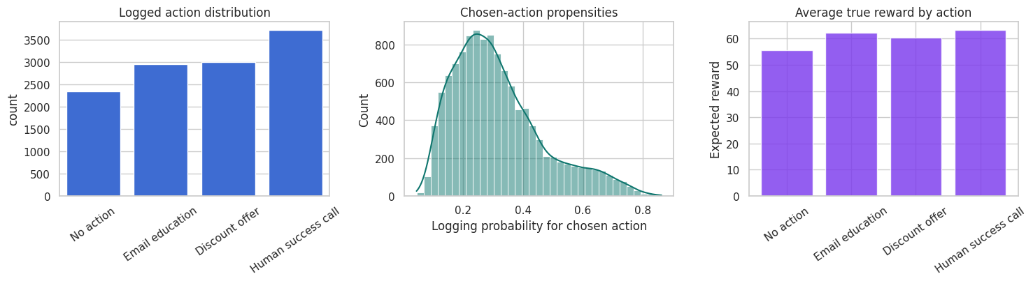
This setup is a contextual bandit:
- The system sees context.
- It chooses one action.
- It observes only that action’s reward.
- The rewards for the unchosen actions are missing.
The logging policy is stochastic and stores propensities. That is the feature that makes reliable OPE possible. If the logs only stored the chosen action and reward, we would have a much weaker evaluation problem.
4. Candidate Target Policies
We will evaluate several target policies:
- Logging policy: the policy that generated the data.
- Uniform random policy: a sanity-check policy.
- Business rule: a transparent hand-built rule.
- Model argmax policy: a deterministic policy that chooses the action with the highest predicted reward.
- Conservative model policy: mostly follows the model argmax but keeps 15% uniform exploration.
- Aggressive call-heavy policy: a riskier policy that uses many human calls.
The model-based policies are learned on a policy-design split. Their values are evaluated on a separate evaluation split.
design_idx, eval_idx = train_test_split(
    df.index,
    test_size=0.45,
    random_state=5710,
    stratify=df["action"],
)
design = df.loc[design_idx].copy()
eval_logs = df.loc[eval_idx].copy()


def fit_action_reward_models(frame, feature_cols):
    models = {}
    base_model = HistGradientBoostingRegressor(
        max_iter=180,
        learning_rate=0.045,
        min_samples_leaf=45,
        l2_regularization=0.03,
        random_state=5711,
    )
    for action_id in range(N_ACTIONS):
        action_frame = frame[frame["action"] == action_id]
        model = clone(base_model)
        model.fit(action_frame[feature_cols], action_frame["reward"])
        models[action_id] = model
    return models


def predict_action_rewards(models, frame, feature_cols):
    preds = np.zeros((len(frame), N_ACTIONS))
    for action_id, model in models.items():
        preds[:, action_id] = model.predict(frame[feature_cols])
    return preds


policy_design_models = fit_action_reward_models(design, feature_cols)
eval_pred_rewards_for_policy = predict_action_rewards(policy_design_models, eval_logs, feature_cols)
model_argmax_actions = eval_pred_rewards_for_policy.argmax(axis=1)


def business_rule_actions(frame):
    action = np.zeros(len(frame), dtype=int)
    call = (frame["enterprise"].to_numpy() == 1) & (frame["churn_risk"].to_numpy() > 0.58)
    discount = (~call) & (frame["price_sensitivity"].to_numpy() > 0.67) & (frame["churn_risk"].to_numpy() > 0.42)
    email = (~call) & (~discount) & (
        (frame["onboarding_gap"].to_numpy() > 0.55) | (frame["email_engagement"].to_numpy() > 0.65)
    )
    action[email] = 1
    action[discount] = 2
    action[call] = 3
    return action


def aggressive_call_actions(frame):
    action = np.ones(len(frame), dtype=int)
    discount = frame["price_sensitivity"].to_numpy() > 0.55
    call = (frame["enterprise"].to_numpy() == 1) | (frame["churn_risk"].to_numpy() > 0.48)
    action[discount] = 2
    action[call] = 3
    return action


def conservative_probs(actions, epsilon=0.15):
    return (1 - epsilon) * one_hot(actions) + epsilon / N_ACTIONS


target_policies = {
    "Logging policy": eval_logs[logging_prob_cols].to_numpy(),
    "Uniform random": np.ones((len(eval_logs), N_ACTIONS)) / N_ACTIONS,
    "Business rule": one_hot(business_rule_actions(eval_logs)),
    "Model argmax": one_hot(model_argmax_actions),
    "Conservative model": conservative_probs(model_argmax_actions, epsilon=0.15),
    "Aggressive call-heavy": one_hot(aggressive_call_actions(eval_logs)),
}

policy_action_mix = []
for policy_name, probs in target_policies.items():
    action_rates = probs.mean(axis=0)
    row = {"policy": policy_name}
    for action_id, label in ACTION_LABELS.items():
        row[label] = action_rates[action_id]
    policy_action_mix.append(row)

display(pd.DataFrame(policy_action_mix))| policy | No action | Email education | Discount offer | Human success call | |
|---|---|---|---|---|---|
| 0 | Logging policy | 0.189 | 0.248 | 0.253 | 0.310 |
| 1 | Uniform random | 0.250 | 0.250 | 0.250 | 0.250 |
| 2 | Business rule | 0.503 | 0.276 | 0.065 | 0.156 |
| 3 | Model argmax | 0.008 | 0.291 | 0.242 | 0.459 |
| 4 | Conservative model | 0.044 | 0.285 | 0.244 | 0.427 |
| 5 | Aggressive call-heavy | 0.000 | 0.204 | 0.092 | 0.704 |
The action mix is an immediate deployment diagnostic. A policy that shifts heavily toward an expensive or operationally scarce action may have a high estimated reward but still be infeasible.
It is also an OPE diagnostic. The more different the target policy is from the logging policy, the harder offline evaluation becomes.
5. Ground Truth Value in Simulation
In real life, policy value is unknown. Here we can compute it because the simulation contains all potential reward means:
\[ V(\pi) = \frac{1}{n} \sum_i \sum_a \pi(a \mid X_i)\mu_a(X_i) \]
where \(\mu_a(X_i)=E[Y_i(a)\mid X_i]\).
This simulation truth lets us separate two questions:
- What does each OPE estimator say?
- How close is that estimate to the value we know from the data-generating process?
def true_policy_value(frame, target_probs):
    return np.mean(np.sum(target_probs * frame[mu_cols].to_numpy(), axis=1))


truth_table = pd.DataFrame(
    [
        {
            "policy": name,
            "true_value": true_policy_value(eval_logs, probs),
            "true_gain_vs_logging": true_policy_value(eval_logs, probs)
            - true_policy_value(eval_logs, target_policies["Logging policy"]),
        }
        for name, probs in target_policies.items()
    ]
).sort_values("true_value", ascending=False)

display(truth_table)| policy | true_value | true_gain_vs_logging | |
|---|---|---|---|
| 3 | Model argmax | 67.325 | 4.533 |
| 4 | Conservative model | 66.276 | 3.484 |
| 5 | Aggressive call-heavy | 65.291 | 2.499 |
| 0 | Logging policy | 62.792 | 0.000 |
| 2 | Business rule | 61.850 | -0.942 |
| 1 | Uniform random | 60.333 | -2.459 |
6. Why Naive Offline Evaluation Fails
A naive matched-outcome estimate keeps only rows where the logged action matches the target policy action and averages their observed rewards.
For deterministic target policies:
\[ \hat{V}_{matched} = \frac{\sum_i 1\{A_i = \pi(X_i)\}R_i} {\sum_i 1\{A_i = \pi(X_i)\}} \]
This can be badly biased when the logging policy is context-dependent. The matched rows are not a random sample of all contexts. They are the contexts where the logging policy happened to take the same action as the target policy.
Proper OPE accounts for the probability of the observed action under the logging policy.
def deterministic_actions_from_probs(probs):
    is_deterministic = np.all((np.isclose(probs, 0) | np.isclose(probs, 1)), axis=1)
    if not np.all(is_deterministic):
        return None
    return probs.argmax(axis=1)


naive_rows = []
for policy_name, probs in target_policies.items():
    target_actions = deterministic_actions_from_probs(probs)
    if target_actions is None:
        continue
    matched = eval_logs["action"].to_numpy() == target_actions
    naive_rows.append(
        {
            "policy": policy_name,
            "matched_share": matched.mean(),
            "naive_matched_reward": eval_logs.loc[matched, "reward"].mean(),
            "true_value": true_policy_value(eval_logs, probs),
            "naive_bias": eval_logs.loc[matched, "reward"].mean() - true_policy_value(eval_logs, probs),
        }
    )

display(pd.DataFrame(naive_rows).sort_values("naive_bias"))| policy | matched_share | naive_matched_reward | true_value | naive_bias | |
|---|---|---|---|---|---|
| 0 | Business rule | 0.323 | 63.967 | 61.850 | 2.117 |
| 1 | Model argmax | 0.402 | 69.657 | 67.325 | 2.332 |
| 2 | Aggressive call-heavy | 0.377 | 69.453 | 65.291 | 4.162 |
The matched-outcome estimator is tempting because it feels like “look at cases where we did the same thing.” But if the old system took that action only for certain kinds of accounts, the matched subset does not represent the population the new policy would touch.
7. OPE Estimators
Let \(p_i = \mu(A_i \mid X_i)\) be the logged propensity of the action actually taken.
Let \(q_i = \pi(A_i \mid X_i)\) be the target policy probability of that same action.
The importance weight is:
\[ w_i = \frac{q_i}{p_i} \]
Inverse propensity scoring estimates:
\[ \hat{V}_{IPS} = \frac{1}{n}\sum_i w_iR_i \]
Self-normalized IPS estimates:
\[ \hat{V}_{SNIPS} = \frac{\sum_i w_iR_i}{\sum_i w_i} \]
The direct method estimates a reward model \(\hat{\mu}_a(x)\) and plugs it in:
\[ \hat{V}_{DM} = \frac{1}{n}\sum_i\sum_a \pi(a \mid X_i)\hat{\mu}_a(X_i) \]
The doubly robust estimator combines both:
\[ \hat{V}_{DR} = \frac{1}{n}\sum_i \left[ \sum_a \pi(a \mid X_i)\hat{\mu}_a(X_i) + \frac{\pi(A_i \mid X_i)}{\mu(A_i \mid X_i)} \{R_i-\hat{\mu}_{A_i}(X_i)\} \right] \]
DR is attractive because the reward model supplies baseline predictions while the weighted residual corrects the model using logged outcomes.
def crossfit_reward_matrix(frame, feature_cols, n_splits=5, seed=5712):
    n = len(frame)
    mu_hat = np.zeros((n, N_ACTIONS))
    fold_id = np.zeros(n, dtype=int)
    base_model = HistGradientBoostingRegressor(
        max_iter=180,
        learning_rate=0.045,
        min_samples_leaf=40,
        l2_regularization=0.025,
        random_state=seed,
    )

    kfold = KFold(n_splits=n_splits, shuffle=True, random_state=seed)
    for fold, (train_idx, test_idx) in enumerate(kfold.split(frame), start=1):
        train = frame.iloc[train_idx]
        test = frame.iloc[test_idx]
        for action_id in range(N_ACTIONS):
            action_train = train[train["action"] == action_id]
            model = clone(base_model)
            model.fit(action_train[feature_cols], action_train["reward"])
            mu_hat[test_idx, action_id] = model.predict(test[feature_cols])
        fold_id[test_idx] = fold
    return mu_hat, fold_id


mu_hat_eval, fold_id_eval = crossfit_reward_matrix(eval_logs, feature_cols)
eval_logs = eval_logs.copy()
eval_logs["fold"] = fold_id_eval

chosen_actions = eval_logs["action"].to_numpy()
chosen_mu_hat = mu_hat_eval[np.arange(len(eval_logs)), chosen_actions]
reward_rmse_chosen = np.sqrt(mean_squared_error(eval_logs["reward"], chosen_mu_hat))
potential_rmse = np.sqrt(mean_squared_error(eval_logs[mu_cols].to_numpy().ravel(), mu_hat_eval.ravel()))

pd.DataFrame(
    {
        "diagnostic": [
            "Out-of-fold reward RMSE on observed actions",
            "Out-of-fold reward RMSE against all simulated potential means",
        ],
        "value": [reward_rmse_chosen, potential_rmse],
    }
)| diagnostic | value | |
|---|---|---|
| 0 | Out-of-fold reward RMSE on observed actions | 7.897 |
| 1 | Out-of-fold reward RMSE against all simulated ... | 3.663 |
def evaluate_ope_estimators(frame, target_probs, mu_hat, logging_probs=None, clip=12.0):
    if logging_probs is None:
        logging_probs = frame[logging_prob_cols].to_numpy()
    action = frame["action"].to_numpy()
    reward = frame["reward"].to_numpy()
    n = len(frame)

    p_chosen = logging_probs[np.arange(n), action]
    q_chosen = target_probs[np.arange(n), action]
    weights = q_chosen / np.clip(p_chosen, 1e-6, None)
    clipped_weights = np.minimum(weights, clip)

    dm_row = np.sum(target_probs * mu_hat, axis=1)
    residual = reward - mu_hat[np.arange(n), action]

    ips_contrib = weights * reward
    clipped_ips_contrib = clipped_weights * reward
    dr_contrib = dm_row + weights * residual
    clipped_dr_contrib = dm_row + clipped_weights * residual

    estimators = {
        "Direct method": dm_row,
        "IPS": ips_contrib,
        "Clipped IPS": clipped_ips_contrib,
        "Doubly robust": dr_contrib,
        "Clipped DR": clipped_dr_contrib,
    }

    rows = []
    for name, contrib in estimators.items():
        rows.append(
            {
                "estimator": name,
                "estimate": np.mean(contrib),
                "std_error": np.std(contrib, ddof=1) / np.sqrt(n),
            }
        )

    if weights.sum() > 0:
        snips_estimate = np.sum(weights * reward) / np.sum(weights)
        snips_if = weights * (reward - snips_estimate) / np.mean(weights)
        rows.append(
            {
                "estimator": "SNIPS",
                "estimate": snips_estimate,
                "std_error": np.std(snips_if, ddof=1) / np.sqrt(n),
            }
        )

    return pd.DataFrame(rows), weights


all_ope_rows = []
weight_rows = []
for policy_name, probs in target_policies.items():
    estimates, weights = evaluate_ope_estimators(eval_logs, probs, mu_hat_eval, clip=12.0)
    truth = true_policy_value(eval_logs, probs)
    estimates["policy"] = policy_name
    estimates["true_value"] = truth
    estimates["bias_vs_truth"] = estimates["estimate"] - truth
    estimates["ci_low"] = estimates["estimate"] - 1.96 * estimates["std_error"]
    estimates["ci_high"] = estimates["estimate"] + 1.96 * estimates["std_error"]
    all_ope_rows.append(estimates)

    weight_rows.append(
        {
            "policy": policy_name,
            "mean_weight": weights.mean(),
            "max_weight": weights.max(),
            "share_zero_weight": np.mean(weights == 0),
            "share_weight_gt_10": np.mean(weights > 10),
            "effective_sample_size": effective_sample_size(weights),
            "ess_fraction": effective_sample_size(weights) / len(weights),
        }
    )

ope_results = pd.concat(all_ope_rows, ignore_index=True)
weight_diagnostics = pd.DataFrame(weight_rows).sort_values("ess_fraction")

display(weight_diagnostics)| policy | mean_weight | max_weight | share_zero_weight | share_weight_gt_10 | effective_sample_size | ess_fraction | |
|---|---|---|---|---|---|---|---|
| 2 | Business rule | 1.048 | 13.851 | 0.677 | 0.001 | 1416.516 | 0.262 |
| 5 | Aggressive call-heavy | 1.013 | 10.549 | 0.623 | 0.000 | 1668.987 | 0.309 |
| 3 | Model argmax | 1.012 | 8.882 | 0.598 | 0.000 | 1939.358 | 0.359 |
| 4 | Conservative model | 1.009 | 7.882 | 0.000 | 0.000 | 2420.539 | 0.448 |
| 1 | Uniform random | 0.991 | 4.620 | 0.000 | 0.000 | 4238.381 | 0.785 |
| 0 | Logging policy | 1.000 | 1.000 | 0.000 | 0.000 | 5400.000 | 1.000 |
The effective sample size is a practical OPE warning light:
\[ ESS = \frac{(\sum_i w_i)^2}{\sum_i w_i^2} \]
A low ESS means the estimate is driven by a small number of heavily weighted observations. In that situation, the point estimate may be unstable even if the dataset is large.
display(
    ope_results[
        ["policy", "estimator", "estimate", "std_error", "ci_low", "ci_high", "true_value", "bias_vs_truth"]
    ].sort_values(["policy", "estimator"])
)| policy | estimator | estimate | std_error | ci_low | ci_high | true_value | bias_vs_truth | |
|---|---|---|---|---|---|---|---|---|
| 34 | Aggressive call-heavy | Clipped DR | 65.115 | 0.327 | 64.475 | 65.756 | 65.291 | -0.176 |
| 32 | Aggressive call-heavy | Clipped IPS | 65.728 | 1.283 | 63.213 | 68.242 | 65.291 | 0.436 |
| 30 | Aggressive call-heavy | Direct method | 65.303 | 0.259 | 64.796 | 65.810 | 65.291 | 0.012 |
| 33 | Aggressive call-heavy | Doubly robust | 65.115 | 0.327 | 64.475 | 65.756 | 65.291 | -0.176 |
| 31 | Aggressive call-heavy | IPS | 65.728 | 1.283 | 63.213 | 68.242 | 65.291 | 0.436 |
| 35 | Aggressive call-heavy | SNIPS | 64.860 | 0.533 | 63.815 | 65.904 | 65.291 | -0.432 |
| 16 | Business rule | Clipped DR | 61.910 | 0.314 | 61.296 | 62.525 | 61.850 | 0.060 |
| 14 | Business rule | Clipped IPS | 63.968 | 1.473 | 61.082 | 66.855 | 61.850 | 2.118 |
| 12 | Business rule | Direct method | 61.787 | 0.223 | 61.349 | 62.224 | 61.850 | -0.064 |
| 15 | Business rule | Doubly robust | 61.912 | 0.314 | 61.297 | 62.526 | 61.850 | 0.061 |
| 13 | Business rule | IPS | 63.992 | 1.475 | 61.101 | 66.883 | 61.850 | 2.141 |
| 17 | Business rule | SNIPS | 61.081 | 0.478 | 60.145 | 62.018 | 61.850 | -0.769 |
| 28 | Conservative model | Clipped DR | 66.319 | 0.272 | 65.786 | 66.853 | 66.276 | 0.043 |
| 26 | Conservative model | Clipped IPS | 67.100 | 1.056 | 65.030 | 69.170 | 66.276 | 0.823 |
| 24 | Conservative model | Direct method | 66.332 | 0.223 | 65.895 | 66.769 | 66.276 | 0.056 |
| 27 | Conservative model | Doubly robust | 66.319 | 0.272 | 65.786 | 66.853 | 66.276 | 0.043 |
| 25 | Conservative model | IPS | 67.100 | 1.056 | 65.030 | 69.170 | 66.276 | 0.823 |
| 29 | Conservative model | SNIPS | 66.505 | 0.357 | 65.806 | 67.205 | 66.276 | 0.229 |
| 4 | Logging policy | Clipped DR | 62.780 | 0.244 | 62.301 | 63.259 | 62.792 | -0.012 |
| 2 | Logging policy | Clipped IPS | 62.813 | 0.254 | 62.315 | 63.311 | 62.792 | 0.021 |
| 0 | Logging policy | Direct method | 62.849 | 0.215 | 62.428 | 63.270 | 62.792 | 0.057 |
| 3 | Logging policy | Doubly robust | 62.780 | 0.244 | 62.301 | 63.259 | 62.792 | -0.012 |
| 1 | Logging policy | IPS | 62.813 | 0.254 | 62.315 | 63.311 | 62.792 | 0.021 |
| 5 | Logging policy | SNIPS | 62.813 | 0.254 | 62.315 | 63.311 | 62.792 | 0.021 |
| 22 | Model argmax | Clipped DR | 67.384 | 0.286 | 66.825 | 67.944 | 67.325 | 0.059 |
| 20 | Model argmax | Clipped IPS | 68.387 | 1.260 | 65.917 | 70.857 | 67.325 | 1.062 |
| 18 | Model argmax | Direct method | 67.382 | 0.228 | 66.935 | 67.828 | 67.325 | 0.056 |
| 21 | Model argmax | Doubly robust | 67.384 | 0.286 | 66.825 | 67.944 | 67.325 | 0.059 |
| 19 | Model argmax | IPS | 68.387 | 1.260 | 65.917 | 70.857 | 67.325 | 1.062 |
| 23 | Model argmax | SNIPS | 67.566 | 0.400 | 66.782 | 68.349 | 67.325 | 0.240 |
| 10 | Uniform random | Clipped DR | 60.284 | 0.243 | 59.808 | 60.760 | 60.333 | -0.049 |
| 8 | Uniform random | Clipped IPS | 59.805 | 0.459 | 58.904 | 60.705 | 60.333 | -0.529 |
| 6 | Uniform random | Direct method | 60.384 | 0.204 | 59.984 | 60.783 | 60.333 | 0.050 |
| 9 | Uniform random | Doubly robust | 60.284 | 0.243 | 59.808 | 60.760 | 60.333 | -0.049 |
| 7 | Uniform random | IPS | 59.805 | 0.459 | 58.904 | 60.705 | 60.333 | -0.529 |
| 11 | Uniform random | SNIPS | 60.368 | 0.271 | 59.836 | 60.900 | 60.333 | 0.035 |
fig, axes = plt.subplots(1, 2, figsize=(15, 5.2))

selected_estimators = ["Direct method", "IPS", "SNIPS", "Doubly robust", "Clipped DR"]
plot_results = ope_results[ope_results["estimator"].isin(selected_estimators)].copy()

sns.scatterplot(
    data=plot_results,
    x="true_value",
    y="estimate",
    hue="estimator",
    style="policy",
    s=85,
    ax=axes[0],
)
min_value = min(plot_results["true_value"].min(), plot_results["estimate"].min()) - 2
max_value = max(plot_results["true_value"].max(), plot_results["estimate"].max()) + 2
axes[0].plot([min_value, max_value], [min_value, max_value], color="#111827", linestyle="--")
axes[0].set_title("OPE estimates versus simulation truth")
axes[0].set_xlabel("True policy value")
axes[0].set_ylabel("Estimated policy value")

bias_plot = plot_results.copy()
bias_plot["policy_estimator"] = bias_plot["policy"] + " | " + bias_plot["estimator"]
sns.barplot(
    data=bias_plot,
    y="policy",
    x="bias_vs_truth",
    hue="estimator",
    ax=axes[1],
)
axes[1].axvline(0, color="#111827", linewidth=1.1)
axes[1].set_title("Estimator bias in the simulation")
axes[1].set_xlabel("Estimate minus true value")
axes[1].set_ylabel("")

plt.tight_layout()
plt.show()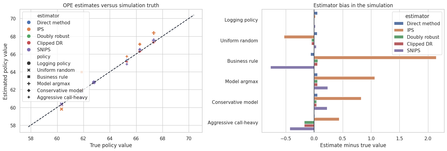
The comparison shows the central OPE tradeoff:
- Direct method can have low variance but can be biased when the reward model is wrong.
- IPS is less model-dependent but can have high variance when target and logging policies disagree.
- SNIPS often stabilizes IPS but introduces small finite-sample bias.
- DR often performs well because it combines a reward model with propensity correction.
- Clipping reduces variance but adds bias.
No estimator dominates in every problem. The best estimator depends on overlap, reward-model quality, action-space size, and how far the target policy moves from the logging policy.
8. Inspecting Importance Weights
Importance weights are the mechanical heart of IPS and DR:
\[ w_i = \frac{\pi(A_i \mid X_i)}{\mu(A_i \mid X_i)} \]
Large weights mean the target policy puts much more probability on the logged action than the logging policy did. Zero weights mean the logged action would not be chosen by the target policy.
Weight diagnostics are not optional. They tell us whether the logged data are informative for the proposed target policy.
weight_plot_rows = []
for policy_name, probs in target_policies.items():
    _, weights = evaluate_ope_estimators(eval_logs, probs, mu_hat_eval, clip=12.0)
    if policy_name in ["Business rule", "Model argmax", "Conservative model", "Aggressive call-heavy"]:
        sample_weights = pd.DataFrame({"policy": policy_name, "weight": weights})
        weight_plot_rows.append(sample_weights)

weight_plot = pd.concat(weight_plot_rows, ignore_index=True)

fig, axes = plt.subplots(1, 2, figsize=(14, 4.8))

sns.histplot(
    data=weight_plot,
    x="weight",
    hue="policy",
    bins=45,
    common_norm=False,
    stat="density",
    alpha=0.38,
    ax=axes[0],
)
axes[0].set_xlim(0, 25)
axes[0].set_title("Importance-weight distributions")
axes[0].set_xlabel("Importance weight")

sns.barplot(
    data=weight_diagnostics,
    y="policy",
    x="ess_fraction",
    color="#2563eb",
    ax=axes[1],
)
axes[1].set_title("Effective sample size fraction")
axes[1].set_xlabel("ESS / n")
axes[1].set_ylabel("")

plt.tight_layout()
plt.show()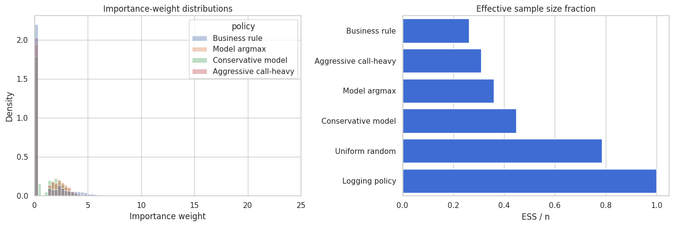
The aggressive policy is the kind of policy that often makes OPE uncomfortable. It may be operationally attractive, but if historical logs rarely used the same actions in similar contexts, then the estimate depends on a thin slice of the data.
An OPE readout should not simply rank policies by point estimate. It should also report whether each estimate is supported by the logs.
9. Clipping Sensitivity
Clipping caps the largest importance weights:
\[ w_i^{clip} = \min(w_i, c) \]
This reduces variance but changes the estimand. A large shift in the estimate across clipping thresholds is a warning that the evaluation is weight-sensitive.
clip_rows = []
clip_grid = [2, 4, 6, 8, 12, 20, 40]
for policy_name in ["Model argmax", "Conservative model", "Aggressive call-heavy"]:
    probs = target_policies[policy_name]
    truth = true_policy_value(eval_logs, probs)
    for clip_value in clip_grid:
        estimates, _ = evaluate_ope_estimators(eval_logs, probs, mu_hat_eval, clip=clip_value)
        subset = estimates[estimates["estimator"].isin(["Clipped IPS", "Clipped DR"])].copy()
        subset["clip"] = clip_value
        subset["policy"] = policy_name
        subset["true_value"] = truth
        clip_rows.append(subset)

clip_df = pd.concat(clip_rows, ignore_index=True)

fig, axes = plt.subplots(1, 2, figsize=(14, 4.8))
for ax, estimator in zip(axes, ["Clipped IPS", "Clipped DR"]):
    sns.lineplot(
        data=clip_df[clip_df["estimator"] == estimator],
        x="clip",
        y="estimate",
        hue="policy",
        marker="o",
        ax=ax,
    )
    for policy_name in ["Model argmax", "Conservative model", "Aggressive call-heavy"]:
        truth = true_policy_value(eval_logs, target_policies[policy_name])
        ax.axhline(truth, color="#64748b", linestyle=":", linewidth=1)
    ax.set_title(f"{estimator} sensitivity to clipping")
    ax.set_xlabel("Weight cap")
    ax.set_ylabel("Estimated policy value")

plt.tight_layout()
plt.show()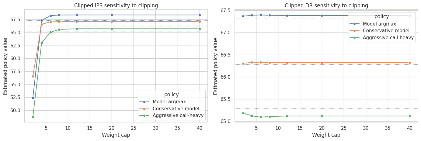
Stable estimates across a reasonable clipping range are reassuring. Large movement is not automatically fatal, but it means the offline estimate should be treated as exploratory rather than launch-ready.
10. Known Versus Estimated Logging Propensities
Production OPE works best when the logging system records the exact action probabilities used at decision time.
If propensities are not logged, analysts may estimate them from historical data. That can be useful, but it adds another nuisance model and another source of bias. Worse, if the old policy was deterministic, the missing support cannot be repaired by estimating propensities after the fact.
Here we estimate the logging policy from the evaluation logs and compare OPE for one target policy using known versus estimated propensities.
def crossfit_logging_propensities(frame, feature_cols, n_splits=5, seed=5713):
    n = len(frame)
    prop_hat = np.zeros((n, N_ACTIONS))
    base_model = HistGradientBoostingClassifier(
        max_iter=180,
        learning_rate=0.045,
        min_samples_leaf=45,
        l2_regularization=0.03,
        random_state=seed,
    )
    kfold = KFold(n_splits=n_splits, shuffle=True, random_state=seed)
    for train_idx, test_idx in kfold.split(frame):
        train = frame.iloc[train_idx]
        test = frame.iloc[test_idx]
        model = clone(base_model)
        model.fit(train[feature_cols], train["action"])
        pred = model.predict_proba(test[feature_cols])
        full_pred = np.zeros((len(test), N_ACTIONS))
        for col_idx, action_id in enumerate(model.classes_):
            full_pred[:, int(action_id)] = pred[:, col_idx]
        prop_hat[test_idx, :] = np.clip(full_pred, 0.02, 0.98)
        prop_hat[test_idx, :] = prop_hat[test_idx, :] / prop_hat[test_idx, :].sum(axis=1, keepdims=True)
    return prop_hat


estimated_logging_probs = crossfit_logging_propensities(eval_logs, feature_cols)
known_logging_probs = eval_logs[logging_prob_cols].to_numpy()

propensity_compare = pd.DataFrame(
    {
        "diagnostic": [
            "Mean absolute propensity error",
            "Log loss using known logging probabilities",
            "Log loss using estimated logging probabilities",
        ],
        "value": [
            np.mean(np.abs(estimated_logging_probs - known_logging_probs)),
            log_loss(eval_logs["action"], known_logging_probs, labels=list(range(N_ACTIONS))),
            log_loss(eval_logs["action"], estimated_logging_probs, labels=list(range(N_ACTIONS))),
        ],
    }
)
display(propensity_compare)| diagnostic | value | |
|---|---|---|
| 0 | Mean absolute propensity error | 0.091 |
| 1 | Log loss using known logging probabilities | 1.258 |
| 2 | Log loss using estimated logging probabilities | 1.384 |
comparison_policy = "Conservative model"
known_estimates, known_weights = evaluate_ope_estimators(
    eval_logs,
    target_policies[comparison_policy],
    mu_hat_eval,
    logging_probs=known_logging_probs,
    clip=12.0,
)
estimated_estimates, estimated_weights = evaluate_ope_estimators(
    eval_logs,
    target_policies[comparison_policy],
    mu_hat_eval,
    logging_probs=estimated_logging_probs,
    clip=12.0,
)

known_estimates["propensity_source"] = "Known logged propensity"
estimated_estimates["propensity_source"] = "Estimated propensity model"
propensity_source_comparison = pd.concat([known_estimates, estimated_estimates], ignore_index=True)
propensity_source_comparison["true_value"] = true_policy_value(eval_logs, target_policies[comparison_policy])
propensity_source_comparison["bias_vs_truth"] = (
    propensity_source_comparison["estimate"] - propensity_source_comparison["true_value"]
)

display(
    propensity_source_comparison[
        ["propensity_source", "estimator", "estimate", "std_error", "true_value", "bias_vs_truth"]
    ]
)| propensity_source | estimator | estimate | std_error | true_value | bias_vs_truth | |
|---|---|---|---|---|---|---|
| 0 | Known logged propensity | Direct method | 66.332 | 0.223 | 66.276 | 0.056 |
| 1 | Known logged propensity | IPS | 67.100 | 1.056 | 66.276 | 0.823 |
| 2 | Known logged propensity | Clipped IPS | 67.100 | 1.056 | 66.276 | 0.823 |
| 3 | Known logged propensity | Doubly robust | 66.319 | 0.272 | 66.276 | 0.043 |
| 4 | Known logged propensity | Clipped DR | 66.319 | 0.272 | 66.276 | 0.043 |
| 5 | Known logged propensity | SNIPS | 66.505 | 0.357 | 66.276 | 0.229 |
| 6 | Estimated propensity model | Direct method | 66.332 | 0.223 | 66.276 | 0.056 |
| 7 | Estimated propensity model | IPS | 80.279 | 1.547 | 66.276 | 14.003 |
| 8 | Estimated propensity model | Clipped IPS | 79.725 | 1.486 | 66.276 | 13.449 |
| 9 | Estimated propensity model | Doubly robust | 66.228 | 0.321 | 66.276 | -0.048 |
| 10 | Estimated propensity model | Clipped DR | 66.187 | 0.310 | 66.276 | -0.089 |
| 11 | Estimated propensity model | SNIPS | 65.662 | 0.414 | 66.276 | -0.615 |
The estimated propensity model is not terrible in this simulation, but it is still inferior to having the true logged propensities. In real systems, logging propensities is a design requirement, not a reporting nicety.
11. Policy Contrast: Is the New Policy Better Than the Current One?
Often the real business question is not “what is the absolute value of policy \(\pi\)?” but:
Is the proposed policy better than the current policy?
For a target policy \(\pi\) and current policy \(\mu\), estimate:
\[ \Delta = V(\pi)-V(\mu) \]
The direct way is to estimate both values and subtract them. The uncertainty can be large because the two estimates are correlated. For a practical first pass, we can compute per-row DR contributions for both policies and take their difference.
def dr_contribution(frame, target_probs, mu_hat, logging_probs=None):
    if logging_probs is None:
        logging_probs = frame[logging_prob_cols].to_numpy()
    action = frame["action"].to_numpy()
    reward = frame["reward"].to_numpy()
    n = len(frame)
    p_chosen = logging_probs[np.arange(n), action]
    q_chosen = target_probs[np.arange(n), action]
    weights = q_chosen / np.clip(p_chosen, 1e-6, None)
    dm_row = np.sum(target_probs * mu_hat, axis=1)
    residual = reward - mu_hat[np.arange(n), action]
    return dm_row + weights * residual


contrast_rows = []
logging_contrib = dr_contribution(eval_logs, target_policies["Logging policy"], mu_hat_eval)
for policy_name in ["Business rule", "Model argmax", "Conservative model", "Aggressive call-heavy"]:
    target_contrib = dr_contribution(eval_logs, target_policies[policy_name], mu_hat_eval)
    contrast = target_contrib - logging_contrib
    contrast_rows.append(
        {
            "policy": policy_name,
            "dr_gain_vs_logging": contrast.mean(),
            "std_error": contrast.std(ddof=1) / np.sqrt(len(contrast)),
            "ci_low": contrast.mean() - 1.96 * contrast.std(ddof=1) / np.sqrt(len(contrast)),
            "ci_high": contrast.mean() + 1.96 * contrast.std(ddof=1) / np.sqrt(len(contrast)),
            "true_gain_vs_logging": true_policy_value(eval_logs, target_policies[policy_name])
            - true_policy_value(eval_logs, target_policies["Logging policy"]),
        }
    )

contrast_table = pd.DataFrame(contrast_rows).sort_values("dr_gain_vs_logging", ascending=False)
display(contrast_table)| policy | dr_gain_vs_logging | std_error | ci_low | ci_high | true_gain_vs_logging | |
|---|---|---|---|---|---|---|
| 1 | Model argmax | 4.605 | 0.144 | 4.322 | 4.887 | 4.533 |
| 2 | Conservative model | 3.539 | 0.119 | 3.306 | 3.772 | 3.484 |
| 3 | Aggressive call-heavy | 2.335 | 0.176 | 1.991 | 2.680 | 2.499 |
| 0 | Business rule | -0.868 | 0.206 | -1.272 | -0.465 | -0.942 |
fig, ax = plt.subplots(figsize=(9, 4.8))
plot_contrast = contrast_table.sort_values("dr_gain_vs_logging")
ax.barh(plot_contrast["policy"], plot_contrast["dr_gain_vs_logging"], color="#2563eb", alpha=0.82)
ax.errorbar(
    x=plot_contrast["dr_gain_vs_logging"],
    y=np.arange(len(plot_contrast)),
    xerr=[
        plot_contrast["dr_gain_vs_logging"] - plot_contrast["ci_low"],
        plot_contrast["ci_high"] - plot_contrast["dr_gain_vs_logging"],
    ],
    fmt="none",
    ecolor="#111827",
    capsize=3,
)
ax.scatter(plot_contrast["true_gain_vs_logging"], np.arange(len(plot_contrast)), color="#dc2626", label="Simulation truth", zorder=5)
ax.axvline(0, color="#111827", linewidth=1.1)
ax.set_title("DR-estimated gain versus logging policy")
ax.set_xlabel("Policy value gain")
ax.legend()
plt.tight_layout()
plt.show()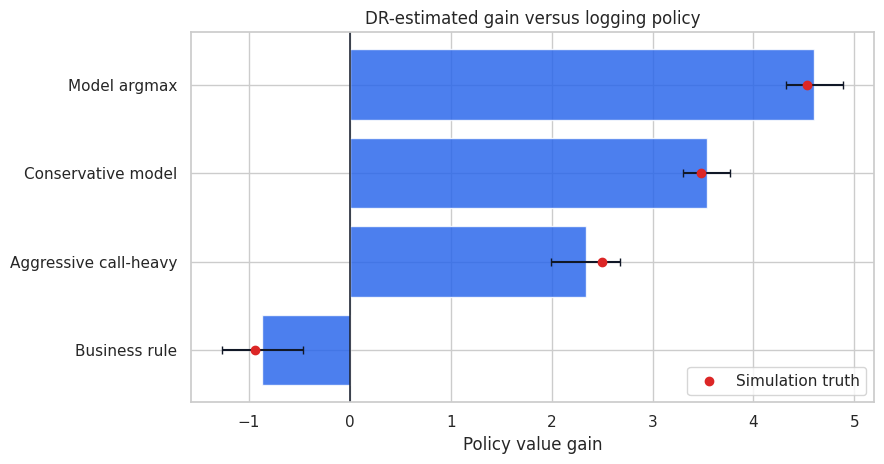
This is the kind of table that belongs in an executive readout. It compares proposed policies to the current baseline, shows uncertainty, and keeps the support diagnostics nearby.
The important move is to avoid treating the highest point estimate as a deployment command. A policy with a slightly lower estimate but much better support may be the better next experiment.
12. Stress Test: What If the Target Policy Is Too Far Away?
OPE is strongest when the target policy is close enough to the logging policy that the logs contain relevant evidence.
If a proposed policy takes actions that the logging policy almost never took for similar contexts, then:
- IPS weights become extreme.
- SNIPS may look stable while estimating a support-limited quantity.
- Direct method relies heavily on extrapolation.
- DR inherits both reward-model risk and weight instability.
In practice, the right next step may be a small randomized exploration pilot, not a full launch.
support_summary = weight_diagnostics.merge(
    truth_table[["policy", "true_gain_vs_logging"]],
    on="policy",
    how="left",
)
support_summary["ope_risk_level"] = pd.cut(
    support_summary["ess_fraction"],
    bins=[-0.01, 0.10, 0.30, 0.60, 1.01],
    labels=["High", "Elevated", "Moderate", "Low"],
)

display(
    support_summary[
        [
            "policy",
            "true_gain_vs_logging",
            "ess_fraction",
            "max_weight",
            "share_weight_gt_10",
            "share_zero_weight",
            "ope_risk_level",
        ]
    ].sort_values("ess_fraction")
)| policy | true_gain_vs_logging | ess_fraction | max_weight | share_weight_gt_10 | share_zero_weight | ope_risk_level | |
|---|---|---|---|---|---|---|---|
| 0 | Business rule | -0.942 | 0.262 | 13.851 | 0.001 | 0.677 | Elevated |
| 1 | Aggressive call-heavy | 2.499 | 0.309 | 10.549 | 0.000 | 0.623 | Moderate |
| 2 | Model argmax | 4.533 | 0.359 | 8.882 | 0.000 | 0.598 | Moderate |
| 3 | Conservative model | 3.484 | 0.448 | 7.882 | 0.000 | 0.000 | Moderate |
| 4 | Uniform random | -2.459 | 0.785 | 4.620 | 0.000 | 0.000 | Low |
| 5 | Logging policy | 0.000 | 1.000 | 1.000 | 0.000 | 0.000 | Low |
13. Industry Readout Template
A professional OPE readout should be explicit about both value and reliability:
- Decision: which target policy is being considered?
- Logged data: time window, eligible population, action set, reward definition, and logging policy.
- Identification: why historical action assignment can be treated as randomized conditional on context.
- Propensities: whether exact propensities were logged or estimated after the fact.
- Estimators: direct method, IPS/SNIPS, DR, and clipped variants.
- Main result: estimated value and gain versus current policy.
- Support diagnostics: ESS, max weights, zero-weight share, and action mix shift.
- Sensitivity: clipping thresholds, reward-model choices, and target-policy stochasticity.
- Recommendation: launch, reject, revise policy, or run an exploration pilot.
Good OPE is not just an estimator. It is a decision-control process for changing deployed systems safely.
recommended_policy = contrast_table.iloc[0]["policy"]
recommended_support = support_summary[support_summary["policy"] == recommended_policy].iloc[0]
recommended_contrast = contrast_table[contrast_table["policy"] == recommended_policy].iloc[0]

readout = pd.DataFrame(
    {
        "item": [
            "Top DR-estimated policy",
            "Estimated gain vs logging",
            "Approximate 95% CI",
            "Simulation true gain vs logging",
            "ESS fraction",
            "Maximum importance weight",
            "OPE risk level",
            "Recommended next step",
        ],
        "value": [
            recommended_policy,
            f"{recommended_contrast['dr_gain_vs_logging']:.2f}",
            f"[{recommended_contrast['ci_low']:.2f}, {recommended_contrast['ci_high']:.2f}]",
            f"{recommended_contrast['true_gain_vs_logging']:.2f}",
            f"{recommended_support['ess_fraction']:.2%}",
            f"{recommended_support['max_weight']:.1f}",
            str(recommended_support["ope_risk_level"]),
            "Use OPE as a screening result, then validate with a randomized pilot.",
        ],
    }
)
display(readout)| item | value | |
|---|---|---|
| 0 | Top DR-estimated policy | Model argmax |
| 1 | Estimated gain vs logging | 4.60 |
| 2 | Approximate 95% CI | [4.32, 4.89] |
| 3 | Simulation true gain vs logging | 4.53 |
| 4 | ESS fraction | 35.91% |
| 5 | Maximum importance weight | 8.9 |
| 6 | OPE risk level | Moderate |
| 7 | Recommended next step | Use OPE as a screening result, then validate w... |
Key Takeaways
- OPE estimates the value of a target policy using data logged under another policy.
- Partial feedback is the central problem: only the chosen action’s reward is observed.
- IPS corrects the action-distribution mismatch with importance weights.
- SNIPS often reduces variance but can introduce finite-sample bias.
- Direct method depends heavily on reward-model quality.
- Doubly robust estimation combines reward modeling with importance-weighted residual correction.
- Weight diagnostics are central. Low ESS and large weights mean the logged data provide weak support.
- Exact logged propensities are a production requirement for reliable OPE.
- Clipping, shrinkage, and stochastic target policies can improve stability, but they change the bias-variance tradeoff.
- OPE should usually screen policies for experimentation, not replace final validation for high-stakes decisions.
References
Dudik, M., Erhan, D., Langford, J., & Li, L. (2014). Doubly robust policy evaluation and optimization. Statistical Science, 29(4), 485-511. https://doi.org/10.1214/14-sts500
Horvitz, D. G., & Thompson, D. J. (1952). A generalization of sampling without replacement from a finite universe. Journal of the American Statistical Association, 47(260), 663-685. https://doi.org/10.1080/01621459.1952.10483446
Saito, Y., & Joachims, T. (2022). Off-policy evaluation for large action spaces via embeddings. arXiv. https://doi.org/10.48550/arxiv.2202.06317
Su, Y., Dimakopoulou, M., Krishnamurthy, A., & Dudik, M. (2019). Doubly robust off-policy evaluation with shrinkage. arXiv. https://doi.org/10.48550/arxiv.1907.09623
Zhan, R., Hadad, V., Hirshberg, D. A., & Athey, S. (2021). Off-policy evaluation via adaptive weighting with data from contextual bandits. arXiv. https://doi.org/10.48550/arxiv.2106.02029