02. CATE and Uplift Modeling

The previous notebook introduced heterogeneous treatment effects and the CATE. This notebook focuses on uplift modeling, the industry-facing version of the same idea when the outcome is often binary: conversion, churn, renewal, click, purchase, activation, or default.

Uplift modeling asks a targeting question: who is more likely to respond because of the treatment? That is different from asking who is likely to convert. A customer can be likely to convert anyway. Another customer can have a modest baseline conversion probability but a large incremental response to the offer.

Learning Goals

By the end of this notebook, you should be able to:

• Explain the relationship between uplift, CATE, and incremental response.
• Distinguish response modeling from uplift modeling.
• Describe the classic uplift segments: persuadables, sure things, lost causes, and sleeping dogs.
• Fit practical uplift scores using two-model, interaction-model, and transformed-outcome approaches.
• Evaluate uplift models with decile lift tables, cumulative uplift curves, AUUC-style summaries, and policy value.
• Explain why ordinary classification metrics can be actively misleading for treatment targeting.

import warnings

import graphviz
import matplotlib.pyplot as plt
import numpy as np
import pandas as pd
import seaborn as sns
from IPython.display import display
from sklearn.ensemble import RandomForestClassifier, RandomForestRegressor
from sklearn.linear_model import LogisticRegression
from sklearn.metrics import average_precision_score, roc_auc_score
from sklearn.model_selection import train_test_split
from sklearn.pipeline import make_pipeline
from sklearn.preprocessing import StandardScaler

warnings.filterwarnings("ignore")

sns.set_theme(style="whitegrid", context="notebook")
pd.set_option("display.float_format", "{:.3f}".format)

def sigmoid(x):
    return 1 / (1 + np.exp(-x))


def make_dag(edges, title=None, node_colors=None, rankdir="LR"):
    graph = graphviz.Digraph(format="svg")
    graph.attr(rankdir=rankdir, bgcolor="white", pad="0.2")
    graph.attr("node", shape="box", style="rounded,filled", color="#334155", fontname="Helvetica")
    graph.attr("edge", color="#475569", arrowsize="0.8")

    node_colors = node_colors or {}
    nodes = sorted({node for edge in edges for node in edge[:2]})
    for node in nodes:
        graph.node(node, fillcolor=node_colors.get(node, "#eef2ff"))

    for edge in edges:
        if len(edge) == 2:
            graph.edge(edge[0], edge[1])
        else:
            graph.edge(edge[0], edge[1], label=edge[2])

    if title:
        graph.attr(label=title, labelloc="t", fontsize="18", fontname="Helvetica-Bold")
    return graph


def simulate_uplift_campaign(n=25_000, seed=5202):
    rng = np.random.default_rng(seed)

    intent_score = rng.beta(2.0, 4.0, n)
    price_sensitivity = rng.beta(2.5, 2.0, n)
    loyalty_score = rng.beta(2.8, 1.8, n)
    visits_30d = rng.poisson(np.clip(1.0 + 7.0 * intent_score, 0.2, None))
    days_since_last_visit = np.clip(rng.gamma(2.0, 10.0, n) * (1.25 - intent_score), 1, 90)
    discount_history = rng.poisson(np.clip(0.3 + 2.4 * price_sensitivity, 0.1, None))
    mobile_app = rng.binomial(1, sigmoid(-0.6 + 1.4 * intent_score + 0.4 * loyalty_score), n)
    annual_contract = rng.binomial(1, sigmoid(-0.5 + 1.7 * loyalty_score - 0.8 * price_sensitivity), n)

    control_logit = (
        -3.4
        + 3.2 * intent_score
        + 1.4 * loyalty_score
        + 0.08 * visits_30d
        - 0.025 * days_since_last_visit
        - 0.75 * price_sensitivity
        + 0.35 * mobile_app
        + 0.45 * annual_contract
    )
    p0 = sigmoid(control_logit)

    raw_uplift = (
        0.16 * price_sensitivity * (1 - loyalty_score)
        + 0.09 * intent_score * price_sensitivity
        + 0.035 * mobile_app
        + 0.025 * (discount_history >= 2).astype(float)
        - 0.10 * loyalty_score * (1 - price_sensitivity)
        - 0.05 * annual_contract * (1 - price_sensitivity)
    )
    p1 = np.clip(p0 + raw_uplift, 0.002, 0.985)
    true_cate = p1 - p0

    treatment = rng.binomial(1, 0.5, n)
    y0 = rng.binomial(1, p0)
    y1 = rng.binomial(1, p1)
    converted = np.where(treatment == 1, y1, y0)

    return pd.DataFrame(
        {
            "customer_id": np.arange(1, n + 1),
            "intent_score": intent_score,
            "price_sensitivity": price_sensitivity,
            "loyalty_score": loyalty_score,
            "visits_30d": visits_30d,
            "days_since_last_visit": days_since_last_visit,
            "discount_history": discount_history,
            "mobile_app": mobile_app,
            "annual_contract": annual_contract,
            "treatment": treatment,
            "converted": converted,
            "p0": p0,
            "p1": p1,
            "true_cate": true_cate,
            "y0": y0,
            "y1": y1,
        }
    )


def top_fraction_mask(frame, score_col, fraction=0.20, largest=True):
    n_select = max(1, int(np.floor(fraction * len(frame))))
    selected_index = frame[score_col].sort_values(ascending=not largest).head(n_select).index
    mask = pd.Series(False, index=frame.index)
    mask.loc[selected_index] = True
    return mask


def response_rate_difference(frame, mask=None, outcome="converted", treatment="treatment"):
    work = frame if mask is None else frame.loc[mask]
    treated = work.loc[work[treatment] == 1, outcome]
    control = work.loc[work[treatment] == 0, outcome]
    estimate = treated.mean() - control.mean()
    se = np.sqrt(treated.var(ddof=1) / treated.size + control.var(ddof=1) / control.size)
    return {
        "n": len(work),
        "n_treated": treated.size,
        "n_control": control.size,
        "treated_rate": treated.mean(),
        "control_rate": control.mean(),
        "observed_uplift": estimate,
        "std_error": se,
        "ci_low": estimate - 1.96 * se,
        "ci_high": estimate + 1.96 * se,
    }


def make_interaction_frame(frame, feature_cols, treatment_value=None):
    base = frame[feature_cols].copy()
    treatment = frame["treatment"].to_numpy() if treatment_value is None else np.repeat(treatment_value, len(frame))
    for col in feature_cols:
        base[f"treat_x_{col}"] = treatment * frame[col].to_numpy()
    base["treatment"] = treatment
    return base


def cumulative_uplift_curve(frame, score_col, outcome="converted", treatment="treatment", propensity=0.5, n_grid=120):
    work = frame.sort_values(score_col, ascending=False).reset_index(drop=True).copy()
    work["ipw_incremental"] = work[outcome] * (
        work[treatment] / propensity - (1 - work[treatment]) / (1 - propensity)
    )
    work["cum_incremental"] = work["ipw_incremental"].cumsum()
    work["contact_share"] = (np.arange(len(work)) + 1) / len(work)
    work["incremental_per_eligible"] = work["cum_incremental"] / len(work)

    grid_idx = np.unique(np.ceil(np.linspace(1, len(work), n_grid)).astype(int) - 1)
    curve = work.loc[grid_idx, ["contact_share", "incremental_per_eligible"]].copy()
    curve = pd.concat(
        [pd.DataFrame({"contact_share": [0.0], "incremental_per_eligible": [0.0]}), curve],
        ignore_index=True,
    )
    curve["incremental_conversions_per_1000"] = 1000 * curve["incremental_per_eligible"]
    return curve


def auuc_from_curve(curve):
    return np.trapezoid(curve["incremental_per_eligible"], curve["contact_share"])


def decile_lift_table(frame, score_col):
    work = frame.sort_values(score_col, ascending=False).reset_index(drop=True).copy()
    labels = [f"D{i} highest" if i == 1 else f"D{i}" for i in range(1, 11)]
    work["score_decile"] = pd.qcut(np.arange(len(work)), q=10, labels=labels)

    rows = []
    for decile, decile_frame in work.groupby("score_decile", observed=True):
        stats = response_rate_difference(decile_frame)
        rows.append(
            {
                "decile": str(decile),
                "n": stats["n"],
                "treated_rate": stats["treated_rate"],
                "control_rate": stats["control_rate"],
                "observed_uplift": stats["observed_uplift"],
                "ci_low": stats["ci_low"],
                "ci_high": stats["ci_high"],
                "true_uplift_mean": decile_frame["true_cate"].mean(),
                "baseline_conversion_mean": decile_frame["p0"].mean(),
            }
        )
    return pd.DataFrame(rows)

1. Uplift Is CATE for a Binary Business Outcome

For a binary outcome, uplift is the incremental probability of success caused by treatment:

\[ Uplift(x) = P(Y=1 \mid do(W=1), X=x) - P(Y=1 \mid do(W=0), X=x) \]

This is the CATE when \(Y\) is binary:

\[ \tau(x) = E[Y(1) - Y(0) \mid X=x] \]

Because \(Y\) is 0 or 1, this is also:

\[ \tau(x) = P(Y(1)=1 \mid X=x) - P(Y(0)=1 \mid X=x) \]

In a randomized experiment, treatment assignment is independent of potential outcomes. That lets us estimate conditional response differences from treatment and control groups. In observational data, the same formulas require stronger assumptions and adjustment for confounding.

make_dag(
    edges=[
        ("CustomerFeatures", "ControlConversionProb"),
        ("CustomerFeatures", "TreatmentConversionProb"),
        ("RandomAssignment", "Treatment"),
        ("Treatment", "ObservedConversion"),
        ("ControlConversionProb", "ObservedConversion"),
        ("TreatmentConversionProb", "ObservedConversion"),
        ("TreatmentConversionProb", "UpliftScore"),
        ("ControlConversionProb", "UpliftScore"),
        ("UpliftScore", "TargetingDecision"),
    ],
    title="Uplift modeling ranks customers by incremental response, not conversion probability alone",
    node_colors={
        "CustomerFeatures": "#dbeafe",
        "RandomAssignment": "#dcfce7",
        "Treatment": "#fee2e2",
        "ControlConversionProb": "#fef3c7",
        "TreatmentConversionProb": "#fef3c7",
        "ObservedConversion": "#f1f5f9",
        "UpliftScore": "#cffafe",
        "TargetingDecision": "#ede9fe",
    },
)

Uplift modeling is common in marketing, lifecycle messaging, ads, churn prevention, recommendations, healthcare outreach, and credit operations. Rzepakowski and Jaroszewicz (2011) describe uplift trees for single and multiple treatments. Soltys et al. (2014) discuss ensemble methods for uplift modeling. Devriendt et al. (2022) frame uplift as a ranking problem, which is often how it is used in production. Betlei et al. (2021) emphasize AUUC-style evaluation for choosing models from randomized experiment data.

2. The Four Uplift Segments

Uplift practitioners often use four conceptual customer types:

• Persuadables: convert only if treated.
• Sure things: convert with or without treatment.
• Lost causes: do not convert either way.
• Sleeping dogs: would convert without treatment but are less likely to convert if treated.

These are not directly observable labels. They are a mental model based on potential outcomes. For a single customer, we observe either \(Y(1)\) or \(Y(0)\), never both. The labels are useful because they clarify why a response model can waste money. A response model tends to find sure things. An uplift model tries to find persuadables and avoid sleeping dogs.

3. Simulated Campaign Data

We will simulate an e-commerce promotion experiment. Half of customers receive a limited-time discount message; half do not. The outcome is whether the customer buys within seven days.

The promotion has three realistic patterns:

• Price-sensitive customers can be persuaded by the discount.
• Highly loyal customers often buy anyway, so their incremental lift is smaller.
• Some loyal annual-contract customers dislike discount messaging, creating negative lift for a small segment.

The true uplift is known only because this is a simulation.

df = simulate_uplift_campaign()

experiment_summary = pd.DataFrame(
    {
        "quantity": [
            "Customers",
            "Treatment share",
            "Observed conversion rate",
            "Control conversion probability, mean",
            "Treatment conversion probability, mean",
            "True average uplift",
            "Share with negative true uplift",
        ],
        "value": [
            len(df),
            df["treatment"].mean(),
            df["converted"].mean(),
            df["p0"].mean(),
            df["p1"].mean(),
            df["true_cate"].mean(),
            (df["true_cate"] < 0).mean(),
        ],
    }
)

display(experiment_summary)
display(df.head())

	quantity	value
0	Customers	25000.000
1	Treatment share	0.505
2	Observed conversion rate	0.218
3	Control conversion probability, mean	0.195
4	Treatment conversion probability, mean	0.238
5	True average uplift	0.043
6	Share with negative true uplift	0.238

	customer_id	intent_score	price_sensitivity	loyalty_score	visits_30d	days_since_last_visit	discount_history	mobile_app	annual_contract	treatment	converted	p0	p1	true_cate	y0	y1
0	1	0.145	0.595	0.785	2	16.761	1	1	0	0	0	0.100	0.132	0.031	0	0
1	2	0.132	0.926	0.537	4	19.831	3	0	1	0	0	0.066	0.163	0.097	0	0
2	3	0.206	0.475	0.763	1	2.755	0	0	1	0	1	0.173	0.133	-0.040	1	0
3	4	0.190	0.532	0.539	1	56.114	2	1	1	0	0	0.049	0.109	0.060	0	0
4	5	0.152	0.289	0.872	2	15.426	1	0	0	1	0	0.106	0.053	-0.052	0	0

The average uplift is the average difference between treatment and control conversion probabilities. In business language, this is the incremental conversion rate caused by the promotion.

A five percentage point uplift can be valuable at scale, but it does not mean every customer should receive the message. Some customers have near-zero or negative lift.

ate_stats = response_rate_difference(df)
ate_table = pd.DataFrame(
    {
        "quantity": [
            "Observed treated conversion rate",
            "Observed control conversion rate",
            "Estimated average uplift",
            "95% CI lower",
            "95% CI upper",
            "True average uplift",
        ],
        "value": [
            ate_stats["treated_rate"],
            ate_stats["control_rate"],
            ate_stats["observed_uplift"],
            ate_stats["ci_low"],
            ate_stats["ci_high"],
            df["true_cate"].mean(),
        ],
    }
)

display(ate_table.round(4))

	quantity	value
0	Observed treated conversion rate	0.239
1	Observed control conversion rate	0.197
2	Estimated average uplift	0.042
3	95% CI lower	0.032
4	95% CI upper	0.052
5	True average uplift	0.043

The randomized experiment recovers the average uplift well. The next question is whether we can rank customers so that the top part of the list has much higher incremental conversion than the average.

fig, axes = plt.subplots(1, 2, figsize=(12, 4.2))

sns.histplot(df["p0"], bins=35, kde=True, color="#2563eb", ax=axes[0])
axes[0].set_title("Baseline conversion probability")
axes[0].set_xlabel("P(Y=1 | control)")

sns.histplot(df["true_cate"], bins=40, kde=True, color="#0f766e", ax=axes[1])
axes[1].axvline(0, color="#334155", linestyle=":")
axes[1].axvline(df["true_cate"].mean(), color="#16a34a", linestyle="--", label="Average uplift")
axes[1].set_title("True uplift distribution")
axes[1].set_xlabel("P(Y=1 | treatment) - P(Y=1 | control)")
axes[1].legend()

plt.tight_layout()
plt.show()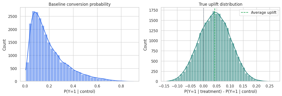

The left plot is about baseline propensity to buy. The right plot is about incremental responsiveness. These are related but not interchangeable.

4. Conceptual Customer Segments in the Simulation

Because we know \(P(Y(0)=1)\) and \(\tau(x)\) in the simulation, we can create approximate teaching labels. These labels are not available in real campaign data, but they make the response-versus-uplift distinction concrete.

def assign_teaching_segment(frame):
    conditions = [
        frame["true_cate"] < -0.015,
        frame["true_cate"] >= 0.085,
        (frame["p0"] >= 0.30) & (frame["true_cate"] < 0.055),
        (frame["p0"] < 0.10) & (frame["true_cate"] < 0.055),
    ]
    choices = ["Sleeping dogs", "Persuadables", "Sure things", "Lost causes"]
    return np.select(conditions, choices, default="Moderate uplift")


df["teaching_segment"] = assign_teaching_segment(df)

segment_table = (
    df.groupby("teaching_segment")
    .agg(
        customers=("customer_id", "count"),
        baseline_conversion=("p0", "mean"),
        treated_conversion=("p1", "mean"),
        true_uplift=("true_cate", "mean"),
        price_sensitivity=("price_sensitivity", "mean"),
        loyalty=("loyalty_score", "mean"),
    )
    .assign(customer_share=lambda x: x["customers"] / len(df))
    .sort_values("true_uplift", ascending=False)
)

display(segment_table.round(3))

plot_sample = df.sample(3500, random_state=22)
fig, ax = plt.subplots(figsize=(8.5, 5.5))
sns.scatterplot(
    data=plot_sample,
    x="p0",
    y="true_cate",
    hue="teaching_segment",
    alpha=0.55,
    edgecolor=None,
    ax=ax,
)
ax.axhline(0, color="#334155", linestyle=":")
ax.set_title("Baseline conversion and uplift are different dimensions")
ax.set_xlabel("Baseline conversion probability")
ax.set_ylabel("True uplift")
ax.legend(title="Teaching segment", bbox_to_anchor=(1.02, 1), loc="upper left")
plt.tight_layout()
plt.show()

	customers	baseline_conversion	treated_conversion	true_uplift	price_sensitivity	loyalty	customer_share
teaching_segment
Persuadables	6017	0.180	0.298	0.118	0.750	0.462	0.241
Moderate uplift	9726	0.181	0.225	0.044	0.570	0.626	0.389
Lost causes	3106	0.064	0.088	0.024	0.530	0.591	0.124
Sure things	2024	0.436	0.456	0.021	0.462	0.713	0.081
Sleeping dogs	4127	0.233	0.189	-0.044	0.308	0.741	0.165

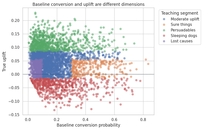
The important contrast is between sure things and persuadables. Sure things have high baseline conversion. Persuadables have high incremental conversion. A campaign that is judged by raw response rate can look good while spending budget on sure things.

5. Train-Test Split and Candidate Scores

We will compare four scoring strategies.

1. Response model: predicts conversion among treated customers. This is common in marketing, but it is not an uplift model.
2. Two-model uplift score: fit one model for treated conversion and one model for control conversion, then subtract probabilities.
3. Interaction model: fit a single classifier with treatment and treatment-feature interactions, then predict each customer twice, once as treated and once as control.
4. Transformed-outcome model: convert each observed row into an unbiased noisy signal of uplift, then regress that signal on features.

The next notebook will go deeper into metalearners. Here the goal is to understand the modeling target and evaluation workflow.

feature_cols = [
    "intent_score",
    "price_sensitivity",
    "loyalty_score",
    "visits_30d",
    "days_since_last_visit",
    "discount_history",
    "mobile_app",
    "annual_contract",
]

strata = df["treatment"].astype(str) + "_" + df["converted"].astype(str)
train_df, test_df = train_test_split(df, test_size=0.40, random_state=19, stratify=strata)

split_summary = pd.DataFrame(
    {
        "sample": ["Train", "Test"],
        "n": [len(train_df), len(test_df)],
        "treatment_share": [train_df["treatment"].mean(), test_df["treatment"].mean()],
        "conversion_rate": [train_df["converted"].mean(), test_df["converted"].mean()],
        "true_average_uplift": [train_df["true_cate"].mean(), test_df["true_cate"].mean()],
    }
)

display(split_summary.round(4))

	sample	n	treatment_share	conversion_rate	true_average_uplift
0	Train	15000	0.505	0.218	0.043
1	Test	10000	0.505	0.218	0.044

# 1. Response model: predicts conversion among treated customers.
response_model = RandomForestClassifier(
    n_estimators=200,
    min_samples_leaf=60,
    random_state=101,
    n_jobs=-1,
)
response_model.fit(
    train_df.loc[train_df["treatment"] == 1, feature_cols],
    train_df.loc[train_df["treatment"] == 1, "converted"],
)

# 2. Two-model uplift score.
treated_model = RandomForestClassifier(
    n_estimators=200,
    min_samples_leaf=60,
    random_state=102,
    n_jobs=-1,
)
control_model = RandomForestClassifier(
    n_estimators=200,
    min_samples_leaf=60,
    random_state=103,
    n_jobs=-1,
)
treated_model.fit(
    train_df.loc[train_df["treatment"] == 1, feature_cols],
    train_df.loc[train_df["treatment"] == 1, "converted"],
)
control_model.fit(
    train_df.loc[train_df["treatment"] == 0, feature_cols],
    train_df.loc[train_df["treatment"] == 0, "converted"],
)

# 3. Single interaction model.
X_train_interaction = make_interaction_frame(train_df, feature_cols)
interaction_model = make_pipeline(
    StandardScaler(),
    LogisticRegression(max_iter=2000, C=0.4),
)
interaction_model.fit(X_train_interaction, train_df["converted"])

# 4. Transformed-outcome model.
propensity = 0.5
transformed_outcome = train_df["converted"] * (
    train_df["treatment"] / propensity - (1 - train_df["treatment"]) / (1 - propensity)
)
transformed_model = RandomForestRegressor(
    n_estimators=200,
    min_samples_leaf=80,
    random_state=104,
    n_jobs=-1,
)
transformed_model.fit(train_df[feature_cols], transformed_outcome)

print("Models fit on randomized treatment-control experiment data.")

Models fit on randomized treatment-control experiment data.

The transformed outcome used above is:

\[ Y_i^* = Y_i\left(\frac{W_i}{e} - \frac{1-W_i}{1-e}\right) \]

where \(e=P(W=1)\). Under random assignment:

\[ E[Y_i^* \mid X_i=x] = E[Y(1)-Y(0) \mid X_i=x] \]

This transformed target is noisy, but it lets us use ordinary regression software to produce an uplift score.

test_scored = test_df.copy()

test_scored["score_response"] = response_model.predict_proba(test_scored[feature_cols])[:, 1]

test_scored["score_two_model"] = (
    treated_model.predict_proba(test_scored[feature_cols])[:, 1]
    - control_model.predict_proba(test_scored[feature_cols])[:, 1]
)

X_test_control = make_interaction_frame(test_scored.assign(treatment=0), feature_cols, treatment_value=0)
X_test_treated = make_interaction_frame(test_scored.assign(treatment=1), feature_cols, treatment_value=1)
test_scored["score_interaction"] = (
    interaction_model.predict_proba(X_test_treated)[:, 1]
    - interaction_model.predict_proba(X_test_control)[:, 1]
)

test_scored["score_transformed"] = transformed_model.predict(test_scored[feature_cols])

display(
    test_scored[
        [
            "customer_id",
            "converted",
            "treatment",
            "p0",
            "true_cate",
            "score_response",
            "score_two_model",
            "score_interaction",
            "score_transformed",
        ]
    ].head(10).round(4)
)

	customer_id	converted	treatment	p0	true_cate	score_response	score_two_model	score_interaction	score_transformed
6933	6934	0	1	0.032	0.127	0.184	0.147	0.068	0.176
14465	14466	0	1	0.118	0.157	0.269	0.085	0.154	0.040
23503	23504	1	0	0.368	-0.030	0.335	-0.047	-0.107	0.108
17025	17026	0	1	0.088	0.129	0.216	0.084	0.104	0.110
22270	22271	0	1	0.513	0.097	0.547	-0.004	0.045	-0.158
2263	2264	0	1	0.133	-0.051	0.097	-0.042	-0.028	-0.035
5420	5421	0	1	0.349	0.048	0.334	-0.040	0.015	-0.021
9292	9293	0	1	0.161	-0.003	0.133	-0.068	0.022	-0.139
15691	15692	0	1	0.133	0.035	0.213	0.055	0.048	0.075
7770	7771	0	0	0.373	0.076	0.376	-0.006	0.077	0.073

Every model produces a score, but the scores mean different things. The response score estimates conversion under treatment. The other three scores estimate incremental conversion caused by treatment.

6. Why Classification Metrics Can Mislead

A response model can have a strong AUC because it predicts who converts when treated. But targeting by this score can still be inefficient if many high-scoring customers would have converted without treatment.

We will compare two kinds of metrics:

• Treated-response AUC and average precision: ordinary predictive metrics among treated customers.
• Uplift usefulness: correlation with true uplift in the simulation, observed uplift in the top 20%, and true mean uplift in the top 20%.

In real data, the true-uplift columns are unavailable. The observed top-bin lift is the practical experimental check.

score_map = {
    "Response model": "score_response",
    "Two-model uplift": "score_two_model",
    "Interaction uplift": "score_interaction",
    "Transformed outcome": "score_transformed",
}

comparison_rows = []
for model_name, score_col in score_map.items():
    top20 = top_fraction_mask(test_scored, score_col, fraction=0.20)
    top20_stats = response_rate_difference(test_scored, top20)
    treated_test = test_scored.loc[test_scored["treatment"] == 1]
    comparison_rows.append(
        {
            "model": model_name,
            "treated_response_auc": roc_auc_score(treated_test["converted"], treated_test[score_col]),
            "treated_average_precision": average_precision_score(treated_test["converted"], treated_test[score_col]),
            "corr_with_true_uplift": np.corrcoef(test_scored[score_col], test_scored["true_cate"])[0, 1],
            "observed_uplift_top20": top20_stats["observed_uplift"],
            "true_uplift_top20": test_scored.loc[top20, "true_cate"].mean(),
            "negative_uplift_share_top20": (test_scored.loc[top20, "true_cate"] < 0).mean(),
        }
    )

comparison_table = pd.DataFrame(comparison_rows).sort_values("true_uplift_top20", ascending=False)
display(comparison_table.round(4))

	model	treated_response_auc	treated_average_precision	corr_with_true_uplift	observed_uplift_top20	true_uplift_top20	negative_uplift_share_top20
2	Interaction uplift	0.492	0.257	0.841	0.069	0.116	0.000
1	Two-model uplift	0.502	0.249	0.752	0.093	0.107	0.003
3	Transformed outcome	0.484	0.260	0.590	0.084	0.100	0.034
0	Response model	0.710	0.448	0.283	0.065	0.061	0.181

The response model can score well on treated-response AUC but still be a weaker targeting rule. The uplift models are not trying to predict conversion. They are trying to predict incremental conversion.

This is the first major habit shift: do not pick an uplift model using ordinary classification accuracy, AUC, or log loss alone.

fig, axes = plt.subplots(1, 2, figsize=(12, 4.6))
plot_sample = test_scored.sample(3000, random_state=35)

sns.scatterplot(
    data=plot_sample,
    x="score_response",
    y="true_cate",
    alpha=0.35,
    edgecolor=None,
    color="#2563eb",
    ax=axes[0],
)
axes[0].set_title("Response score does not rank uplift cleanly")
axes[0].set_xlabel("Predicted conversion if treated")
axes[0].set_ylabel("True uplift")

sns.scatterplot(
    data=plot_sample,
    x="score_interaction",
    y="true_cate",
    alpha=0.35,
    edgecolor=None,
    color="#0f766e",
    ax=axes[1],
)
axes[1].set_title("Interaction uplift score tracks incremental lift")
axes[1].set_xlabel("Predicted uplift")
axes[1].set_ylabel("True uplift")

plt.tight_layout()
plt.show()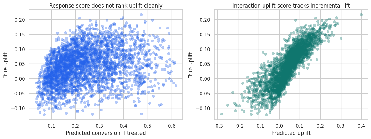

The response score is strongly related to baseline conversion. The uplift score is more directly related to incremental response. This distinction is the reason uplift modeling exists.

7. Decile Lift Tables

A decile table is often the most practical way to explain uplift results to stakeholders. Sort customers by the model score, split them into ten equally sized groups, and estimate treatment-control lift inside each group.

For a useful uplift model, the top deciles should have much higher observed treatment-control differences than the lower deciles.

interaction_deciles = decile_lift_table(test_scored, "score_interaction")
display(interaction_deciles.round(4))

fig, ax = plt.subplots(figsize=(9.5, 4.8))
y = np.arange(len(interaction_deciles))
ax.errorbar(
    interaction_deciles["observed_uplift"],
    y,
    xerr=np.vstack(
        [
            interaction_deciles["observed_uplift"] - interaction_deciles["ci_low"],
            interaction_deciles["ci_high"] - interaction_deciles["observed_uplift"],
        ]
    ),
    fmt="o",
    color="#2563eb",
    ecolor="#94a3b8",
    capsize=4,
    label="Observed treatment-control lift",
)
ax.scatter(
    interaction_deciles["true_uplift_mean"],
    y,
    color="#dc2626",
    marker="D",
    label="True mean uplift",
)
ax.axvline(0, color="#334155", linestyle=":")
ax.set_yticks(y)
ax.set_yticklabels(interaction_deciles["decile"])
ax.set_xlabel("Incremental conversion rate")
ax.set_title("Decile lift table for the interaction uplift model")
ax.invert_yaxis()
ax.legend(loc="best")
plt.tight_layout()
plt.show()

	decile	n	treated_rate	control_rate	observed_uplift	ci_low	ci_high	true_uplift_mean	baseline_conversion_mean
0	D1 highest	1000	0.299	0.195	0.104	0.051	0.157	0.133	0.201
1	D2	1000	0.263	0.229	0.034	-0.019	0.088	0.100	0.177
2	D3	1000	0.249	0.167	0.082	0.032	0.132	0.081	0.158
3	D4	1000	0.206	0.146	0.061	0.014	0.108	0.065	0.148
4	D5	1000	0.191	0.151	0.039	-0.007	0.086	0.052	0.143
5	D6	1000	0.184	0.132	0.051	0.006	0.097	0.036	0.133
6	D7	1000	0.168	0.132	0.037	-0.008	0.081	0.017	0.142
7	D8	1000	0.186	0.182	0.004	-0.045	0.052	-0.002	0.178
8	D9	1000	0.253	0.251	0.002	-0.052	0.056	-0.013	0.261
9	D10	1000	0.392	0.388	0.005	-0.056	0.065	-0.033	0.412

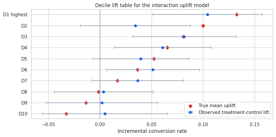
The top deciles show high incremental conversion. Lower deciles are weaker and may include customers who should not receive the promotion.

In real applications, this table should be computed on a holdout experiment or on future randomized traffic. It should not be trusted if it is computed on the same data used to tune many competing models.

8. Cumulative Uplift Curves and AUUC

A cumulative uplift curve asks: if we contact the top \(k\) percent of customers according to the score, how many incremental conversions do we estimate?

For a randomized experiment with treatment probability \(e\), an inverse-probability weighted estimate of incremental conversions in a selected set \(S\) is:

\[ \widehat{\Delta}(S) = \sum_{i \in S} Y_i\left(\frac{W_i}{e} - \frac{1-W_i}{1-e}\right) \]

Dividing by the total number of eligible customers gives incremental conversions per eligible customer. Multiplying by 1000 gives incremental conversions per 1000 eligible customers.

The area under this curve is an AUUC-style summary. Larger is better for ranking customers by incremental response.

curve_frames = []
auuc_rows = []
for model_name, score_col in score_map.items():
    curve = cumulative_uplift_curve(test_scored, score_col)
    curve["model"] = model_name
    curve_frames.append(curve)
    auuc_rows.append({"model": model_name, "auuc": auuc_from_curve(curve)})

# Oracle curve is available only in the simulation.
oracle_curve = cumulative_uplift_curve(test_scored, "true_cate")
oracle_curve["model"] = "Oracle true uplift"
curve_frames.append(oracle_curve)
auuc_rows.append({"model": "Oracle true uplift", "auuc": auuc_from_curve(oracle_curve)})

curves = pd.concat(curve_frames, ignore_index=True)
auuc_table = pd.DataFrame(auuc_rows).sort_values("auuc", ascending=False)

overall_curve_end = cumulative_uplift_curve(test_scored.assign(random_score=0.0), "random_score")[
    "incremental_per_eligible"
].iloc[-1]
random_baseline = pd.DataFrame(
    {
        "contact_share": np.linspace(0, 1, 121),
        "incremental_per_eligible": np.linspace(0, overall_curve_end, 121),
    }
)
random_baseline["incremental_conversions_per_1000"] = 1000 * random_baseline["incremental_per_eligible"]
random_baseline["model"] = "Random targeting baseline"

display(auuc_table.round(5))

fig, ax = plt.subplots(figsize=(9.5, 5.5))
sns.lineplot(
    data=pd.concat([curves, random_baseline], ignore_index=True),
    x="contact_share",
    y="incremental_conversions_per_1000",
    hue="model",
    ax=ax,
)
ax.set_title("Cumulative uplift curves on the test experiment")
ax.set_xlabel("Share of eligible customers contacted")
ax.set_ylabel("Incremental conversions per 1000 eligible customers")
ax.legend(title="Score", bbox_to_anchor=(1.02, 1), loc="upper left")
plt.tight_layout()
plt.show()

	model	auuc
4	Oracle true uplift	0.039
1	Two-model uplift	0.034
2	Interaction uplift	0.033
0	Response model	0.029
3	Transformed outcome	0.028

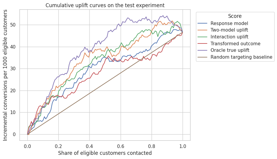
The curve is more informative than a single metric. A model can be excellent in the top 10% and mediocre after that, which is fine if campaign capacity is 10%. If capacity is 60%, a different model may be preferred.

Devriendt et al. (2022) note that uplift modeling is fundamentally a ranking problem. Betlei et al. (2021) discuss AUUC as a model-selection criterion when the future policy treats the highest-scored individuals.

9. Policy Value With Margin and Cost

Incremental conversion is not enough. Campaigns have value and cost.

Suppose one incremental conversion is worth 80 dollars in contribution margin, and each contacted customer costs 5 dollars in discount expense, messaging, or customer-experience risk.

For a selected group \(S\), the true expected net value per eligible customer is:

\[ \frac{|S|}{N}\left(E[\tau(X) \mid X \in S] \times margin - cost\right) \]

In real data, the true uplift term is unavailable, so we use randomized holdout estimates and continue experimenting.

def policy_value_table(frame, score_map, fractions, margin=80.0, contact_cost=5.0, propensity=0.5):
    rows = []
    for model_name, score_col in score_map.items():
        for fraction in fractions:
            mask = top_fraction_mask(frame, score_col, fraction=fraction)
            selected = frame.loc[mask].copy()
            ipw_incremental = selected["converted"] * (
                selected["treatment"] / propensity - (1 - selected["treatment"]) / (1 - propensity)
            )
            rows.append(
                {
                    "model": model_name,
                    "contact_share": fraction,
                    "true_uplift_targeted": selected["true_cate"].mean(),
                    "observed_uplift_targeted": ipw_incremental.mean(),
                    "true_net_value_per_eligible": fraction
                    * (selected["true_cate"].mean() * margin - contact_cost),
                    "observed_net_value_per_eligible": fraction
                    * (ipw_incremental.mean() * margin - contact_cost),
                    "negative_uplift_share_targeted": (selected["true_cate"] < 0).mean(),
                }
            )
    return pd.DataFrame(rows)


fractions = [0.10, 0.20, 0.30, 0.50, 1.00]
policy_scores = {
    "Response model": "score_response",
    "Two-model uplift": "score_two_model",
    "Interaction uplift": "score_interaction",
    "Transformed outcome": "score_transformed",
    "Oracle true uplift": "true_cate",
}
policy_table = policy_value_table(test_scored, policy_scores, fractions)

display(
    policy_table.sort_values(["contact_share", "true_net_value_per_eligible"], ascending=[True, False]).round(4)
)

	model	contact_share	true_uplift_targeted	observed_uplift_targeted	true_net_value_per_eligible	observed_net_value_per_eligible	negative_uplift_share_targeted
20	Oracle true uplift	0.100	0.145	0.126	0.663	0.508	0.000
10	Interaction uplift	0.100	0.133	0.122	0.560	0.476	0.000
5	Two-model uplift	0.100	0.119	0.134	0.453	0.572	0.001
15	Transformed outcome	0.100	0.109	0.124	0.375	0.492	0.024
0	Response model	0.100	0.059	0.062	-0.030	-0.004	0.197
21	Oracle true uplift	0.200	0.126	0.130	1.008	1.080	0.000
11	Interaction uplift	0.200	0.116	0.090	0.860	0.440	0.000
6	Two-model uplift	0.200	0.107	0.108	0.707	0.728	0.003
16	Transformed outcome	0.200	0.100	0.092	0.597	0.472	0.034
1	Response model	0.200	0.061	0.085	-0.029	0.360	0.181
22	Oracle true uplift	0.300	0.112	0.115	1.181	1.252	0.000
12	Interaction uplift	0.300	0.104	0.087	1.006	0.580	0.000
7	Two-model uplift	0.300	0.097	0.101	0.818	0.932	0.007
17	Transformed outcome	0.300	0.089	0.063	0.648	0.020	0.048
2	Response model	0.300	0.059	0.076	-0.079	0.324	0.179
23	Oracle true uplift	0.500	0.091	0.085	1.131	0.892	0.000
13	Interaction uplift	0.500	0.086	0.072	0.948	0.364	0.005
8	Two-model uplift	0.500	0.080	0.076	0.704	0.556	0.027
18	Transformed outcome	0.500	0.074	0.068	0.447	0.204	0.078
3	Response model	0.500	0.060	0.070	-0.095	0.300	0.167
4	Response model	1.000	0.044	0.047	-1.510	-1.272	0.237
9	Two-model uplift	1.000	0.044	0.047	-1.510	-1.272	0.237
14	Interaction uplift	1.000	0.044	0.047	-1.510	-1.272	0.237
19	Transformed outcome	1.000	0.044	0.047	-1.510	-1.272	0.237
24	Oracle true uplift	1.000	0.044	0.047	-1.510	-1.272	0.237

fig, axes = plt.subplots(1, 2, figsize=(13, 5))

sns.lineplot(
    data=policy_table,
    x="contact_share",
    y="true_net_value_per_eligible",
    hue="model",
    marker="o",
    ax=axes[0],
)
axes[0].axhline(0, color="#334155", linestyle=":")
axes[0].set_title("True net value by contact share")
axes[0].set_xlabel("Share contacted")
axes[0].set_ylabel("Net value per eligible customer")

sns.lineplot(
    data=policy_table,
    x="contact_share",
    y="negative_uplift_share_targeted",
    hue="model",
    marker="o",
    ax=axes[1],
)
axes[1].set_title("Share of contacted customers with negative uplift")
axes[1].set_xlabel("Share contacted")
axes[1].set_ylabel("Negative uplift share")
axes[1].legend_.remove()

plt.tight_layout()
plt.show()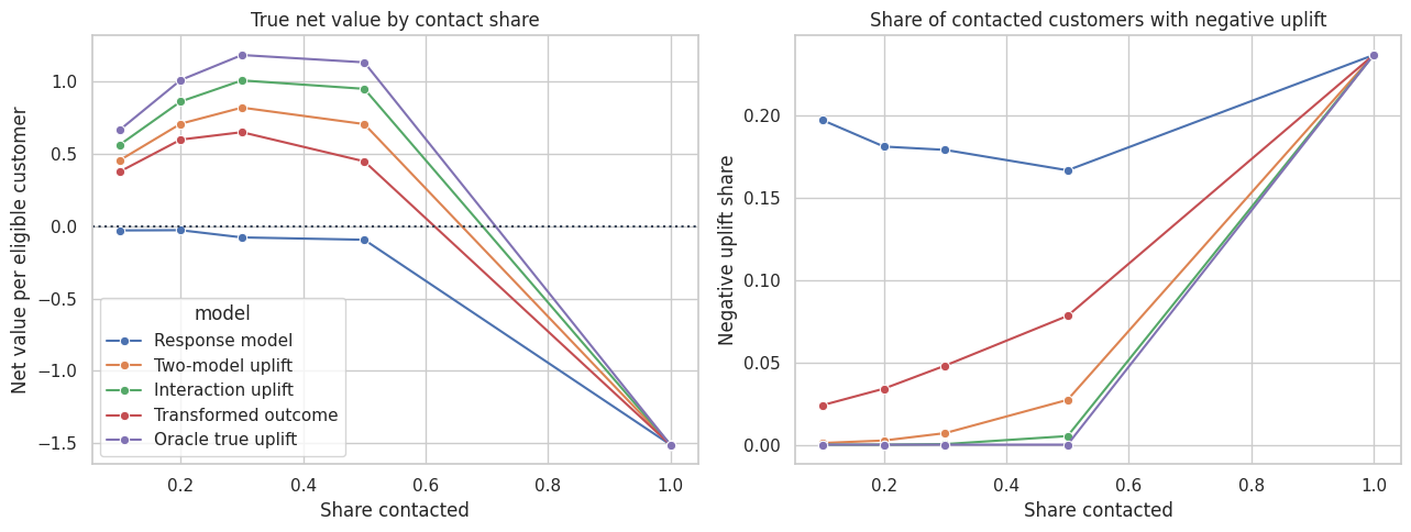

The interaction uplift model creates more value than the response model at constrained contact shares. The response model often contacts customers with high conversion probability, but some of those customers are sure things.

The negative-uplift plot is a useful guardrail. It tells us whether a targeting rule is accidentally contacting many sleeping dogs.

10. Overlap Between Response Targeting and Uplift Targeting

A common stakeholder question is: “Are we really targeting different customers?” We can answer by comparing the top lists.

top20_response = top_fraction_mask(test_scored, "score_response", fraction=0.20)
top20_uplift = top_fraction_mask(test_scored, "score_interaction", fraction=0.20)

test_scored["top20_response_model"] = top20_response
_test_overlap = test_scored.copy()
_test_overlap["top20_interaction_uplift"] = top20_uplift
_test_overlap["targeting_group"] = np.select(
    [
        top20_response & top20_uplift,
        top20_response & ~top20_uplift,
        ~top20_response & top20_uplift,
    ],
    ["Both lists", "Response only", "Uplift only"],
    default="Neither top list",
)

overlap_table = (
    _test_overlap.groupby("targeting_group")
    .agg(
        customers=("customer_id", "count"),
        baseline_conversion=("p0", "mean"),
        true_uplift=("true_cate", "mean"),
        price_sensitivity=("price_sensitivity", "mean"),
        loyalty_score=("loyalty_score", "mean"),
        negative_uplift_share=("true_cate", lambda x: (x < 0).mean()),
    )
    .assign(customer_share=lambda x: x["customers"] / len(_test_overlap))
    .sort_values("true_uplift", ascending=False)
)

display(overlap_table.round(4))

	customers	baseline_conversion	true_uplift	price_sensitivity	loyalty_score	negative_uplift_share	customer_share
targeting_group
Both lists	630	0.305	0.126	0.734	0.519	0.000	0.063
Uplift only	1370	0.136	0.112	0.729	0.473	0.000	0.137
Response only	1370	0.466	0.031	0.497	0.713	0.264	0.137
Neither top list	6630	0.141	0.024	0.522	0.623	0.302	0.663

The “response only” group tends to have stronger baseline conversion than incremental lift. The “uplift only” group is often more price-sensitive and less certain to buy without treatment. This is exactly the strategic difference between conversion prediction and uplift modeling.

11. Practical Modeling Notes

Several implementation details matter in real projects:

• Keep a randomized holdout. Without it, uplift validation becomes fragile.
• Use pre-treatment features only. Post-treatment behavior can leak mediators or outcomes into the model.
• Check treatment and control counts in top bins. Tiny cells produce noisy lift estimates.
• Evaluate at the contact share the business can actually use.
• Include contact costs, margin, opt-outs, and support load in policy value.
• Report uncertainty in top-bin lift, not only point estimates.
• Monitor drift. A model trained on one campaign can decay when pricing, seasonality, audience mix, or offer design changes.
• Avoid claiming individual-level truth. Uplift is usually reliable at ranked-group or segment level, not as a literal person-by-person causal fact.

Uplift modeling is most credible when it is embedded in an experimentation program: learn from randomized treatment-control data, deploy to a constrained audience, and keep randomized exploration so the model can be audited and improved.

12. Industry Readout Template

A good uplift readout for a promotion or retention campaign might include:

1. Average lift: treatment increased conversion by the experimental treatment-control difference.
2. Targeting objective: maximize incremental conversions per contacted customer, not raw conversion rate.
3. Recommended score: use the uplift score, not the treated-response score.
4. Capacity decision: contact the top 20% or 30%, depending on marginal net value.
5. Avoided waste: the response model over-targets sure things; the uplift model finds more persuadables.
6. Risk control: exclude bins with negative or near-zero lift unless there is another strategic reason to contact them.
7. Validation plan: keep a randomized holdout and report decile lift after launch.

This makes the analysis legible to marketing, product, finance, and data science at the same time.

best_fraction = 0.20
readout_rows = []
for model_name in ["Response model", "Interaction uplift", "Oracle true uplift"]:
    row = policy_table.loc[
        (policy_table["model"] == model_name) & (policy_table["contact_share"] == best_fraction)
    ].iloc[0]
    readout_rows.append(
        {
            "targeting_rule": model_name,
            "contact_share": best_fraction,
            "true_uplift_targeted": row["true_uplift_targeted"],
            "true_net_value_per_eligible": row["true_net_value_per_eligible"],
            "negative_uplift_share_targeted": row["negative_uplift_share_targeted"],
        }
    )

readout_table = pd.DataFrame(readout_rows)
display(readout_table.round(4))

	targeting_rule	contact_share	true_uplift_targeted	true_net_value_per_eligible	negative_uplift_share_targeted
0	Response model	0.200	0.061	-0.029	0.181
1	Interaction uplift	0.200	0.116	0.860	0.000
2	Oracle true uplift	0.200	0.126	1.008	0.000

The interaction uplift rule is not perfect, but it moves the campaign in the right direction. It gets closer to the oracle rule than the response model because it is solving the correct causal ranking problem.

Key Takeaways

• Uplift for a binary outcome is the CATE expressed as an incremental probability of success.
• Response modeling asks who will convert; uplift modeling asks whose conversion probability changes because of treatment.
• Sure things can make a campaign look good while wasting treatment budget.
• A response model can have good AUC and still be a weak targeting rule.
• Decile lift tables and cumulative uplift curves are practical tools for model evaluation.
• AUUC-style metrics summarize ranking quality, but business decisions should still use campaign capacity, margin, cost, and guardrails.
• The most credible uplift systems keep randomized holdouts so targeting performance can be measured after deployment.

References

Betlei, A., Diemert, E., & Amini, M.-R. (2021). Uplift modeling with generalization guarantees. Proceedings of the 27th ACM SIGKDD Conference on Knowledge Discovery & Data Mining, 55-65. https://doi.org/10.1145/3447548.3467395

Devriendt, F., Van Belle, J., & Guns, T. (2022). Learning to rank for uplift modeling. IEEE Transactions on Knowledge and Data Engineering, 34(10), 4888-4904. https://doi.org/10.1109/TKDE.2020.3048510

Kunzel, S. R., Sekhon, J. S., Bickel, P. J., & Yu, B. (2019). Metalearners for estimating heterogeneous treatment effects using machine learning. Proceedings of the National Academy of Sciences, 116(10), 4156-4165. https://doi.org/10.1073/pnas.1804597116

Olaya, D., Coussement, K., & Verbeke, W. (2020). A survey and benchmarking study of multitreatment uplift modeling. Data Mining and Knowledge Discovery, 34(2), 273-308. https://doi.org/10.1007/s10618-019-00670-y

Rzepakowski, P., & Jaroszewicz, S. (2011). Decision trees for uplift modeling with single and multiple treatments. Knowledge and Information Systems, 32(2), 303-327. https://doi.org/10.1007/s10115-011-0434-0

Soltys, M., Jaroszewicz, S., & Rzepakowski, P. (2014). Ensemble methods for uplift modeling. Data Mining and Knowledge Discovery, 29(6), 1531-1559. https://doi.org/10.1007/s10618-014-0383-9