05. Clustered Experiments

Many real experiments cannot randomize individual users independently. A delivery marketplace might randomize cities, a retail chain might randomize stores, a sales platform might randomize account teams, and a hospital system might randomize clinics. In each case, the treatment is assigned to a cluster of units.

Clustered experiments are powerful because they let us test interventions that are operationally, socially, or technically delivered at a group level. They are dangerous because the data can look much larger than the experiment really is. Ten thousand users nested inside 40 stores is not the same as ten thousand independently randomized users.

The central idea of this notebook is:

In a clustered experiment, the number of independent randomization units is closer to the number of clusters than the number of rows in the dataset.

That does not mean individual-level data are useless. Individual-level data help define metrics, adjust for pre-treatment covariates, diagnose heterogeneity, and improve precision. But the design and inference must respect the cluster randomization.

Learning Goals

By the end of this notebook, you should be able to:

• Explain why teams randomize stores, schools, clinics, sellers, markets, accounts, or regions instead of individual users.
• Distinguish the unit of randomization, unit of observation, unit of analysis, and target estimand.
• Define intracluster correlation and explain why it reduces effective sample size.
• Compute and interpret the cluster design effect.
• Compare naive user-level inference with cluster-aware inference.
• Show why adding more users inside the same clusters has diminishing returns.
• Diagnose problems caused by few clusters and unequal cluster sizes.
• Decide when to use cluster-level aggregation, cluster-robust standard errors, blocking, or pair matching.
• Write an industry-facing experiment plan for a clustered rollout.

import warnings
warnings.filterwarnings("ignore")

import numpy as np
import pandas as pd
import matplotlib.pyplot as plt
import seaborn as sns
from scipy import stats
import statsmodels.formula.api as smf
from graphviz import Digraph
from IPython.display import display

sns.set_theme(style="whitegrid", context="notebook")
rng = np.random.default_rng(20260428)

COLORS = {
    "assignment": "#d7ecff",
    "cluster": "#ffe0c2",
    "individual": "#dff0d8",
    "outcome": "#eadcf8",
    "warning": "#fff1c7",
    "decision": "#ffd6db",
    "neutral": "#f7f7f7",
    "analysis": "#e1f3ef",
}

def make_dag(edges, title=None, node_colors=None, rankdir="LR"):
    """Create a Graphviz diagram with consistent lecture styling."""
    node_colors = node_colors or {}
    dot = Digraph(format="svg")
    dot.attr(rankdir=rankdir, bgcolor="transparent", pad="0.15", nodesep="0.55", ranksep="0.70")
    dot.attr(
        "node",
        shape="box",
        style="rounded,filled",
        color="#2b2b2b",
        fontname="Helvetica",
        fontsize="11",
        margin="0.12,0.08",
    )
    dot.attr("edge", color="#404040", arrowsize="0.75", penwidth="1.6", fontname="Helvetica", fontsize="10")
    if title:
        dot.attr(label=title, labelloc="t", fontsize="14", fontname="Helvetica-Bold")
    nodes = sorted(set([node for edge in edges for node in edge[:2]]))
    for node in nodes:
        dot.node(node, fillcolor=node_colors.get(node, COLORS["neutral"]))
    for edge in edges:
        if len(edge) == 2:
            src, dst = edge
            dot.edge(src, dst)
        elif len(edge) == 3:
            src, dst, label = edge
            dot.edge(src, dst, label=label)
    return dot


def design_effect(avg_cluster_size, icc):
    """Cluster design effect for equal-sized clusters."""
    return 1 + (avg_cluster_size - 1) * icc


def effective_sample_size(n_units, avg_cluster_size, icc):
    return n_units / design_effect(avg_cluster_size, icc)


def estimate_icc_anova(df, cluster_col, y_col):
    """One-way ANOVA estimate of the intracluster correlation."""
    grouped = df.groupby(cluster_col)[y_col]
    sizes = grouped.size()
    means = grouped.mean()
    grand_mean = df[y_col].mean()
    k = sizes.shape[0]
    n = sizes.sum()
    ss_between = (sizes * (means - grand_mean) ** 2).sum()
    ss_within = grouped.apply(lambda x: ((x - x.mean()) ** 2).sum()).sum()
    ms_between = ss_between / (k - 1)
    ms_within = ss_within / (n - k)
    n_bar = (n - (sizes.pow(2).sum() / n)) / (k - 1)
    return (ms_between - ms_within) / (ms_between + (n_bar - 1) * ms_within)


def plot_ci_table(table, title, xlabel, reference=None, figsize=(8.5, 4.0)):
    ordered = table.sort_values("estimate")
    fig, ax = plt.subplots(figsize=figsize)
    y = np.arange(len(ordered))
    ax.errorbar(
        ordered["estimate"],
        y,
        xerr=[ordered["estimate"] - ordered["ci_low"], ordered["ci_high"] - ordered["estimate"]],
        fmt="o",
        color="#2f6f9f",
        ecolor="#2f6f9f",
        elinewidth=2,
        capsize=4,
    )
    if reference is not None:
        ax.axvline(reference, color="#b23b3b", linestyle="--", linewidth=2, label="True effect")
        ax.legend(loc="lower right")
    ax.axvline(0, color="#333333", linewidth=1)
    ax.set_yticks(y)
    ax.set_yticklabels(ordered["method"])
    ax.set_xlabel(xlabel)
    ax.set_title(title)
    plt.tight_layout()
    plt.show()

1. What Is a Clustered Experiment?

A clustered experiment randomizes groups of units rather than individual units. The cluster may be a store, market, classroom, clinic, village, team, seller, employer, account, region, warehouse, or device fleet.

Concept	Meaning	Example
Unit of randomization	The unit assigned to treatment or control	Store
Unit of observation	The row level in the analysis dataset	Customer visit
Unit of treatment delivery	Where the intervention is implemented	Store-level staffing policy
Unit of decision	The business level where the decision is made	Roll out policy to all stores
Target estimand	The causal effect the team wants to learn	Average effect per customer visit or per store

The hard part is that these units are not always the same. If stores are randomized but customer visits are rows, the rows inside one store share the same assignment and often share unobserved store-level factors. This creates dependence inside clusters.

cluster_edges = [
    ("Cluster assignment", "Store A"),
    ("Cluster assignment", "Store B"),
    ("Cluster assignment", "Store C"),
    ("Store A", "Customers in A"),
    ("Store B", "Customers in B"),
    ("Store C", "Customers in C"),
    ("Store environment", "Customers in A"),
    ("Store environment", "Customers in B"),
    ("Store environment", "Customers in C"),
    ("Customers in A", "Outcomes"),
    ("Customers in B", "Outcomes"),
    ("Customers in C", "Outcomes"),
]
cluster_colors = {
    "Cluster assignment": COLORS["assignment"],
    "Store A": COLORS["cluster"],
    "Store B": COLORS["cluster"],
    "Store C": COLORS["cluster"],
    "Store environment": COLORS["warning"],
    "Customers in A": COLORS["individual"],
    "Customers in B": COLORS["individual"],
    "Customers in C": COLORS["individual"],
    "Outcomes": COLORS["outcome"],
}

display(make_dag(cluster_edges, "Cluster assignment creates grouped outcome data", cluster_colors))

Interpretation

The experiment has many customer rows, but treatment assignment varies only at the store level. Customers in the same store are exposed to the same treatment status and the same store environment. If we analyze each customer row as if it were independently randomized, we usually make the uncertainty look too small.

2. Why Randomize Clusters?

Cluster randomization is not a statistical luxury. In industry settings, it is often the only credible design.

Common reasons include:

Reason	Industry example	Why individual randomization is hard
Contamination	Sales representatives use a new playbook	One representative cannot use two playbooks with different customers cleanly
Operational delivery	Store layout, training, staffing, routing	The treatment is implemented at the store or site level
Spillovers	Marketplace incentives, search ranking, pricing	One user’s treatment can change another user’s experience
Compliance	Account manager workflow, clinical protocol	Individual-level assignment may be ignored or impossible
Fairness and communication	School, workplace, regional policy	Mixed treatment inside a visible group may be unacceptable
Infrastructure	Cache policy, warehouse process, fraud-review queue	Systems may switch at the queue, market, or fleet level

Cluster-randomized trials are common when interventions are delivered to groups, but the design requires explicit attention to within-cluster correlation and the number of available clusters (Campbell et al., 2004; Kennedy-Shaffer & Hughes, 2021). Imai, King, and Nall (2009) use examples such as households, communities, firms, medical practices, schools, and classrooms to describe this basic design feature.

3. Intracluster Correlation

The intracluster correlation coefficient, usually written as $ ho$, measures how similar units are inside the same cluster.

One simple variance-components model is:

\[ Y_{ij} = \mu + u_j + \epsilon_{ij}, \]

where \(i\) indexes individuals and \(j\) indexes clusters. The cluster effect is \(u_j\) and the individual-level noise is \(\epsilon_{ij}\). If:

\[ u_j \sim (0, \sigma_u^2), \qquad \epsilon_{ij} \sim (0, \sigma_\epsilon^2), \]

then the intracluster correlation is:

\[ \rho = \frac{\sigma_u^2}{\sigma_u^2 + \sigma_\epsilon^2}. \]

When \(\rho = 0\), observations in the same cluster are no more similar than observations in different clusters. When \(\rho\) is positive, each additional user inside an existing cluster provides less new information than a user from a new cluster. Campbell et al. (2004) describe the same issue as non-independence of observations within clusters, and Peerawaranun et al. (2019) describe ICC as a measure of response correlation within the same cluster.

cluster_sizes = [5, 20, 50, 100, 250]
icc_values = [0.00, 0.01, 0.03, 0.05, 0.10, 0.20]

de_rows = []
for m in cluster_sizes:
    for icc in icc_values:
        de_rows.append({
            "avg_cluster_size": m,
            "icc": icc,
            "design_effect": design_effect(m, icc),
            "effective_n_from_10000_rows": effective_sample_size(10_000, m, icc),
        })

de_table = pd.DataFrame(de_rows)
de_table.pivot(index="avg_cluster_size", columns="icc", values="design_effect").round(2)

icc	0.00	0.01	0.03	0.05	0.10	0.20
avg_cluster_size
5	1.0	1.04	1.12	1.20	1.4	1.8
20	1.0	1.19	1.57	1.95	2.9	4.8
50	1.0	1.49	2.47	3.45	5.9	10.8
100	1.0	1.99	3.97	5.95	10.9	20.8
250	1.0	3.49	8.47	13.45	25.9	50.8

heatmap_data = de_table.pivot(index="avg_cluster_size", columns="icc", values="design_effect")
fig, ax = plt.subplots(figsize=(8.5, 4.5))
sns.heatmap(
    heatmap_data,
    annot=True,
    fmt=".2f",
    cmap="YlGnBu",
    cbar_kws={"label": "Design effect"},
    ax=ax,
)
ax.set_title("Design effect grows with cluster size and ICC")
ax.set_xlabel("Intracluster correlation")
ax.set_ylabel("Average cluster size")
plt.tight_layout()
plt.show()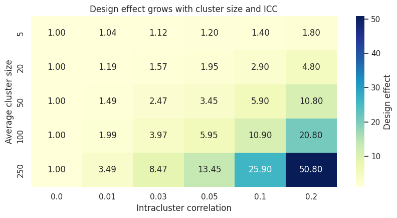

Interpretation

The equal-cluster design effect is:

\[ DE = 1 + (m - 1)\rho, \]

where \(m\) is the average cluster size. This formula appears widely in discussions of cluster-randomized trials; Campbell et al. (2004) use the same expression to describe the loss of effective sample size.

The heatmap shows why even a small ICC matters. If \(m = 100\) and \(\rho = 0.05\), the design effect is \(5.95\). Ten thousand rows then have roughly the information content of only:

\[ \frac{10000}{5.95} \approx 1681 \]

independent observations.

The practical message is uncomfortable but useful: a clustered experiment can have many rows and still have low precision.

4. Simulating a Cluster-Randomized Business Experiment

Now suppose a retail company wants to test a new store-level merchandising policy. The policy is implemented by store managers, so the company randomizes stores. Customer visits are the observation rows.

The true data-generating process has:

• Store-level randomization.
• Store-level baseline differences.
• Customer-level prior demand.
• A constant treatment effect.
• Positive within-store correlation.

We will compare three analyses:

1. Naive user-row analysis: treats customer visits as independent.
2. Cluster-robust regression: keeps user rows but clusters the standard error by store.
3. Cluster-level aggregation: analyzes one row per store.

def simulate_store_experiment(
    n_clusters=80,
    avg_cluster_size=90,
    cluster_size_cv=0.35,
    treatment_effect=1.20,
    icc=0.08,
    individual_sd=4.0,
    seed=20260428,
):
    local_rng = np.random.default_rng(seed)
    cluster_ids = np.arange(n_clusters)
    sigma_cluster = np.sqrt(icc / (1 - icc)) * individual_sd

    raw_sizes = local_rng.lognormal(
        mean=np.log(avg_cluster_size) - 0.5 * cluster_size_cv**2,
        sigma=cluster_size_cv,
        size=n_clusters,
    )
    sizes = np.maximum(25, np.round(raw_sizes)).astype(int)

    treatment_clusters = local_rng.choice(cluster_ids, size=n_clusters // 2, replace=False)
    treatment = np.isin(cluster_ids, treatment_clusters).astype(int)

    store_effect = local_rng.normal(0, sigma_cluster, size=n_clusters)
    store_quality = local_rng.normal(0, 1, size=n_clusters)

    rows = []
    for cluster_id, n, z, u, quality in zip(cluster_ids, sizes, treatment, store_effect, store_quality):
        prior_demand = local_rng.normal(0, 1, size=n)
        pre_metric = 52 + 2.2 * quality + 3.0 * prior_demand + u + local_rng.normal(0, individual_sd, size=n)
        outcome = 55 + 2.2 * quality + 3.0 * prior_demand + u + treatment_effect * z + local_rng.normal(0, individual_sd, size=n)
        rows.append(pd.DataFrame({
            "cluster_id": cluster_id,
            "customer_id": np.arange(n),
            "treatment": z,
            "store_quality": quality,
            "prior_demand": prior_demand,
            "pre_metric": pre_metric,
            "outcome": outcome,
            "cluster_size": n,
        }))

    return pd.concat(rows, ignore_index=True)


df_store = simulate_store_experiment()
print(f"Customer rows: {len(df_store):,}")
print(f"Stores: {df_store['cluster_id'].nunique():,}")
print(f"Average rows per store: {df_store.groupby('cluster_id').size().mean():.1f}")
print(f"Treatment share of stores: {df_store.groupby('cluster_id')['treatment'].first().mean():.2f}")
df_store.head()

Customer rows: 6,648
Stores: 80
Average rows per store: 83.1
Treatment share of stores: 0.50

	cluster_id	customer_id	treatment	store_quality	prior_demand	pre_metric	outcome	cluster_size
0	0	0	1	0.981246	1.800923	57.454616	62.758592	48
1	0	1	1	0.981246	1.297015	59.528463	60.719544	48
2	0	2	1	0.981246	-0.554235	52.979913	53.474985	48
3	0	3	1	0.981246	0.788067	57.428419	56.169411	48
4	0	4	1	0.981246	-0.458051	59.278808	57.253801	48

store_summary = (
    df_store.groupby(["cluster_id", "treatment"], as_index=False)
    .agg(
        outcome_mean=("outcome", "mean"),
        pre_metric_mean=("pre_metric", "mean"),
        cluster_size=("outcome", "size"),
        prior_demand_mean=("prior_demand", "mean"),
    )
)

fig, axes = plt.subplots(1, 2, figsize=(12, 4.5))
sns.histplot(data=store_summary, x="cluster_size", bins=20, color="#2f6f9f", ax=axes[0])
axes[0].set_title("Cluster sizes vary across stores")
axes[0].set_xlabel("Customer visits per store")

sns.scatterplot(
    data=store_summary,
    x="pre_metric_mean",
    y="outcome_mean",
    hue="treatment",
    size="cluster_size",
    sizes=(30, 180),
    palette={0: "#6b7280", 1: "#2f6f9f"},
    ax=axes[1],
)
axes[1].set_title("Store-level outcomes retain store-level structure")
axes[1].set_xlabel("Pre-period store mean")
axes[1].set_ylabel("Experiment-period store mean")
axes[1].legend(title="Treatment", loc="best")
plt.tight_layout()
plt.show()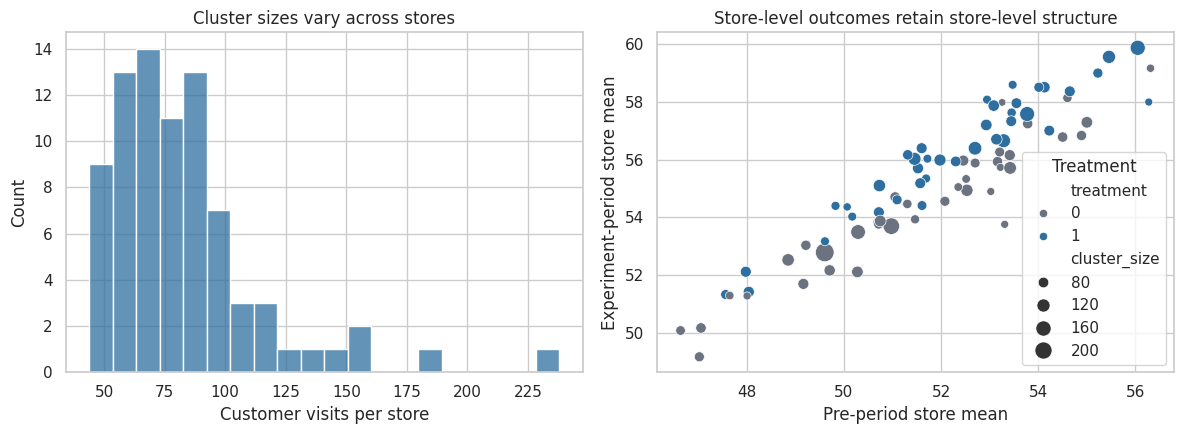

Interpretation

The dataset looks like a large customer-level experiment, but the scatterplot reminds us that the randomized units are stores. Each dot is one independent assignment unit. Store-level baseline differences persist into the outcome period, which is exactly why rows within a store are correlated.

control_only = df_store.query("treatment == 0")
estimated_icc = estimate_icc_anova(control_only, "cluster_id", "outcome")
avg_m = df_store.groupby("cluster_id").size().mean()
print(f"Estimated ICC among control stores: {estimated_icc:.3f}")
print(f"Average cluster size: {avg_m:.1f}")
print(f"Approximate design effect: {design_effect(avg_m, estimated_icc):.2f}")
print(f"Rows: {len(df_store):,}")
print(f"Approximate effective sample size: {effective_sample_size(len(df_store), avg_m, estimated_icc):,.0f}")

Estimated ICC among control stores: 0.149
Average cluster size: 83.1
Approximate design effect: 13.27
Rows: 6,648
Approximate effective sample size: 501

Interpretation

The estimated ICC will vary by simulation, but it is positive. That means a customer row inside a store is not as informative as a customer row from a new independently randomized store. The effective sample size calculation is only an approximation, especially with unequal cluster sizes, but it gives the right intuition.

5. Naive vs Cluster-Aware Inference

The treatment effect estimate can be similar across methods while the standard error changes substantially. This distinction is important.

Randomization protects the point estimate when the design is valid. Clustering mainly changes the uncertainty around that estimate. Cameron and Miller (2015) frame cluster-robust inference as regression inference where errors may be correlated within clusters but independent across clusters. Desai et al. (2013) similarly emphasize that ignoring clustering can distort standard errors and therefore confidence intervals and tests.

def readout_cluster_experiment(df):
    naive_model = smf.ols("outcome ~ treatment", data=df).fit(cov_type="HC1")
    cluster_model = smf.ols("outcome ~ treatment", data=df).fit(
        cov_type="cluster",
        cov_kwds={"groups": df["cluster_id"]},
    )

    cluster_df = (
        df.groupby(["cluster_id", "treatment"], as_index=False)
        .agg(outcome=("outcome", "mean"), n=("outcome", "size"), pre_metric=("pre_metric", "mean"))
    )
    cluster_level_model = smf.ols("outcome ~ treatment", data=cluster_df).fit(cov_type="HC1")
    weighted_cluster_model = smf.wls("outcome ~ treatment", data=cluster_df, weights=cluster_df["n"]).fit(cov_type="HC1")

    models = [
        ("Naive user-row HC1", naive_model),
        ("User-row regression, clustered SE", cluster_model),
        ("Cluster means, unweighted", cluster_level_model),
        ("Cluster means, user-weighted", weighted_cluster_model),
    ]
    rows = []
    for method, model in models:
        est = model.params["treatment"]
        se = model.bse["treatment"]
        rows.append({
            "method": method,
            "estimate": est,
            "se": se,
            "ci_low": est - 1.96 * se,
            "ci_high": est + 1.96 * se,
            "p_value": model.pvalues["treatment"],
        })
    return pd.DataFrame(rows)

readout_table = readout_cluster_experiment(df_store)
readout_table.round(4)

	method	estimate	se	ci_low	ci_high	p_value
0	Naive user-row HC1	2.1706	0.1333	1.9094	2.4318	0.0000
1	User-row regression, clustered SE	2.1706	0.4820	1.2259	3.1153	0.0000
2	Cluster means, unweighted	1.8025	0.4960	0.8303	2.7746	0.0003
3	Cluster means, user-weighted	2.1706	0.4850	1.2199	3.1213	0.0000

plot_ci_table(
    readout_table,
    title="Same point estimate, different uncertainty story",
    xlabel="Estimated treatment effect on customer outcome",
    reference=1.20,
    figsize=(9, 4.2),
)

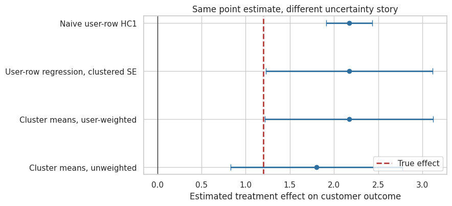
Interpretation

The naive user-row analysis usually reports the smallest standard error because it behaves as if every customer row were an independently randomized unit. The cluster-aware analyses recognize that assignment occurred at the store level.

The cluster-robust approach is often convenient because it keeps individual rows and allows individual-level covariates. The cluster-level approach is often useful as a transparent diagnostic because it shows the experiment’s independent units directly. In practice, it is common to report a regression with cluster-robust standard errors and also sanity-check the result using cluster-level summaries.

6. Adding More Users Inside the Same Clusters Has Diminishing Returns

In an individually randomized experiment, doubling the number of independent users roughly reduces standard errors by a factor of \(\sqrt{2}\). In a clustered experiment, adding more users inside the same stores helps, but the benefit slows down when ICC is positive.

For a fixed number of clusters \(G\) and equal cluster size \(m\):

\[ N = Gm, \]

and the effective sample size is approximately:

\[ N_{eff} = \frac{Gm}{1 + (m - 1)\rho}. \]

As \(m\) gets large, \(N_{eff}\) approaches roughly \(G / \rho\). The ceiling is driven by the number of clusters and the ICC.

cluster_count = 60
m_grid = np.arange(5, 401, 5)
icc_grid = [0.00, 0.01, 0.03, 0.08, 0.15]
curve_rows = []
for icc in icc_grid:
    for m in m_grid:
        total_n = cluster_count * m
        curve_rows.append({
            "avg_cluster_size": m,
            "icc": icc,
            "total_rows": total_n,
            "effective_n": effective_sample_size(total_n, m, icc),
        })
curve_df = pd.DataFrame(curve_rows)

fig, ax = plt.subplots(figsize=(9, 5))
for icc in icc_grid:
    part = curve_df.query("icc == @icc")
    ax.plot(part["avg_cluster_size"], part["effective_n"], linewidth=2.2, label=f"ICC = {icc:.2f}")
ax.set_title("More rows per cluster help less when ICC is positive")
ax.set_xlabel("Average rows per cluster")
ax.set_ylabel("Approximate effective sample size")
ax.legend(title="Within-cluster correlation")
plt.tight_layout()
plt.show()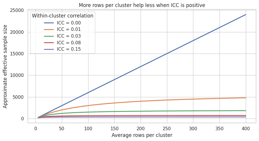

Interpretation

When \(\rho = 0\), effective sample size grows linearly with rows. When \(\rho > 0\), the curves bend. After some point, the better design move is usually to add clusters rather than add more users inside the same clusters.

This is one of the most important design conversations for industry experiments. If a company can choose between 20 stores with many visits and 80 stores with fewer visits each, the second design may be much more informative, even with fewer total rows.

7. Few Clusters Can Break Otherwise Reasonable Analyses

Clustered experiments need enough clusters. With very few clusters, standard large-sample approximations can be fragile. Taljaard et al. (2016) focus specifically on risks that arise when cluster-randomized and stepped-wedge designs have only a small number of clusters. Cameron and Miller (2015) also discuss problems with cluster-robust inference when the number of clusters is small.

A simple simulation makes the point. We set the true treatment effect to zero and repeat the experiment many times. A valid 5% test should reject about 5% of the time.

def one_null_cluster_trial(n_clusters=20, units_per_cluster=80, icc=0.08, seed=None):
    local_rng = np.random.default_rng(seed)
    cluster_ids = np.arange(n_clusters)
    treated_clusters = local_rng.choice(cluster_ids, size=n_clusters // 2, replace=False)
    z_cluster = np.isin(cluster_ids, treated_clusters).astype(int)

    unit_sd = 4.0
    sigma_cluster = np.sqrt(icc / (1 - icc)) * unit_sd
    cluster_effect = local_rng.normal(0, sigma_cluster, size=n_clusters)

    rows = []
    for cluster_id, z, u in zip(cluster_ids, z_cluster, cluster_effect):
        y = 50 + u + local_rng.normal(0, unit_sd, size=units_per_cluster)
        rows.append(pd.DataFrame({"cluster_id": cluster_id, "treatment": z, "outcome": y}))
    df = pd.concat(rows, ignore_index=True)

    naive_p = stats.ttest_ind(
        df.loc[df["treatment"] == 1, "outcome"],
        df.loc[df["treatment"] == 0, "outcome"],
        equal_var=False,
    ).pvalue

    cluster_means = df.groupby(["cluster_id", "treatment"], as_index=False)["outcome"].mean()
    cluster_p = stats.ttest_ind(
        cluster_means.loc[cluster_means["treatment"] == 1, "outcome"],
        cluster_means.loc[cluster_means["treatment"] == 0, "outcome"],
        equal_var=False,
    ).pvalue
    return naive_p, cluster_p

sim_rows = []
for n_clusters in [8, 12, 20, 60]:
    for sim in range(800):
        naive_p, cluster_p = one_null_cluster_trial(
            n_clusters=n_clusters,
            units_per_cluster=80,
            icc=0.08,
            seed=10_000 * n_clusters + sim,
        )
        sim_rows.append({
            "clusters": n_clusters,
            "method": "Naive user-row t-test",
            "reject": naive_p < 0.05,
        })
        sim_rows.append({
            "clusters": n_clusters,
            "method": "Cluster-level t-test",
            "reject": cluster_p < 0.05,
        })

false_positive_df = pd.DataFrame(sim_rows)
false_positive_summary = (
    false_positive_df.groupby(["clusters", "method"], as_index=False)["reject"]
    .mean()
    .rename(columns={"reject": "false_positive_rate"})
)
false_positive_summary.pivot(index="clusters", columns="method", values="false_positive_rate").round(3)

method	Cluster-level t-test	Naive user-row t-test
clusters
8	0.048	0.464
12	0.059	0.472
20	0.049	0.501
60	0.058	0.486

fig, ax = plt.subplots(figsize=(9, 4.7))
sns.barplot(
    data=false_positive_summary,
    x="clusters",
    y="false_positive_rate",
    hue="method",
    palette=["#b23b3b", "#2f6f9f"],
    ax=ax,
)
ax.axhline(0.05, color="#333333", linestyle="--", linewidth=1.5, label="Nominal 5%")
ax.set_title("Ignoring clusters inflates false positives under the null")
ax.set_xlabel("Number of randomized clusters")
ax.set_ylabel("False-positive rate")
ax.legend(loc="upper right")
plt.tight_layout()
plt.show()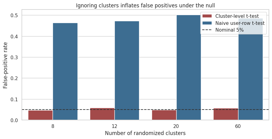

Interpretation

The naive test over-rejects because it counts many correlated user rows as if they were independent. The cluster-level test is not perfect in every small-sample setting, but it is much closer to the design. The main lesson is not that cluster-level t-tests are always the final answer. The lesson is that the effective evidence comes from independently randomized clusters.

When the number of clusters is small, analysts often need small-sample corrections, randomization inference, permutation tests at the cluster level, or wild cluster bootstrap methods. The exact choice depends on the design and the inferential target.

8. Unequal Cluster Sizes Change the Estimand Conversation

Clustered experiments often have unequal cluster sizes. One region may have many more users than another. One enterprise account may have many more seats than another. One store may have much more traffic than another.

This creates an estimand question:

Estimand	Informal meaning	Weighting
Cluster-weighted effect	Effect for the average cluster	Each cluster gets equal weight
User-weighted effect	Effect for the average user or visit	Larger clusters get more weight

Neither estimand is automatically right. A marketplace may care about the average transaction, while an operations team may care about the average site. The problem is failing to say which one is being estimated.

def simulate_unequal_cluster_estimands(seed=20260429):
    local_rng = np.random.default_rng(seed)
    n_clusters = 70
    cluster_ids = np.arange(n_clusters)
    sizes = np.round(local_rng.lognormal(mean=np.log(120), sigma=0.85, size=n_clusters)).astype(int)
    sizes = np.clip(sizes, 20, 700)
    log_size_z = (np.log(sizes) - np.log(sizes).mean()) / np.log(sizes).std()
    tau_cluster = 0.90 + 0.35 * log_size_z
    baseline_cluster = local_rng.normal(0, 2.5, size=n_clusters)

    treated_clusters = local_rng.choice(cluster_ids, size=n_clusters // 2, replace=False)
    z_cluster = np.isin(cluster_ids, treated_clusters).astype(int)

    rows = []
    potential_cluster = []
    for cluster_id, n, z, tau, base in zip(cluster_ids, sizes, z_cluster, tau_cluster, baseline_cluster):
        x = local_rng.normal(0, 1, size=n)
        y0 = 40 + base + 2.0 * x + local_rng.normal(0, 4.0, size=n)
        y1 = y0 + tau
        y = np.where(z == 1, y1, y0)
        rows.append(pd.DataFrame({
            "cluster_id": cluster_id,
            "treatment": z,
            "outcome": y,
            "cluster_size": n,
            "true_cluster_effect": tau,
        }))
        potential_cluster.append({
            "cluster_id": cluster_id,
            "cluster_size": n,
            "true_cluster_effect": tau,
            "treatment": z,
        })
    return pd.concat(rows, ignore_index=True), pd.DataFrame(potential_cluster)


df_unequal, cluster_truth = simulate_unequal_cluster_estimands()
cluster_observed = df_unequal.groupby(["cluster_id", "treatment"], as_index=False).agg(
    outcome=("outcome", "mean"),
    cluster_size=("outcome", "size"),
    true_cluster_effect=("true_cluster_effect", "first"),
)

true_cluster_weighted = cluster_truth["true_cluster_effect"].mean()
true_user_weighted = np.average(cluster_truth["true_cluster_effect"], weights=cluster_truth["cluster_size"])
observed_cluster_weighted = (
    cluster_observed.query("treatment == 1")["outcome"].mean()
    - cluster_observed.query("treatment == 0")["outcome"].mean()
)
observed_user_weighted = (
    df_unequal.query("treatment == 1")["outcome"].mean()
    - df_unequal.query("treatment == 0")["outcome"].mean()
)

estimand_table = pd.DataFrame({
    "quantity": [
        "True cluster-weighted ATE",
        "True user-weighted ATE",
        "Observed cluster-weighted difference",
        "Observed user-weighted difference",
    ],
    "value": [true_cluster_weighted, true_user_weighted, observed_cluster_weighted, observed_user_weighted],
})
estimand_table.round(3)

	quantity	value
0	True cluster-weighted ATE	0.900
1	True user-weighted ATE	1.148
2	Observed cluster-weighted difference	0.561
3	Observed user-weighted difference	0.927

fig, axes = plt.subplots(1, 2, figsize=(12, 4.5))
sns.scatterplot(
    data=cluster_truth,
    x="cluster_size",
    y="true_cluster_effect",
    hue="treatment",
    size="cluster_size",
    sizes=(25, 180),
    palette={0: "#6b7280", 1: "#2f6f9f"},
    ax=axes[0],
)
axes[0].set_title("Larger clusters have different effects in this simulation")
axes[0].set_xlabel("Cluster size")
axes[0].set_ylabel("True cluster-specific effect")
axes[0].legend(title="Treatment", loc="best")

sns.histplot(data=cluster_truth, x="cluster_size", bins=25, color="#2f6f9f", ax=axes[1])
axes[1].set_title("Cluster sizes are highly unequal")
axes[1].set_xlabel("Cluster size")
plt.tight_layout()
plt.show()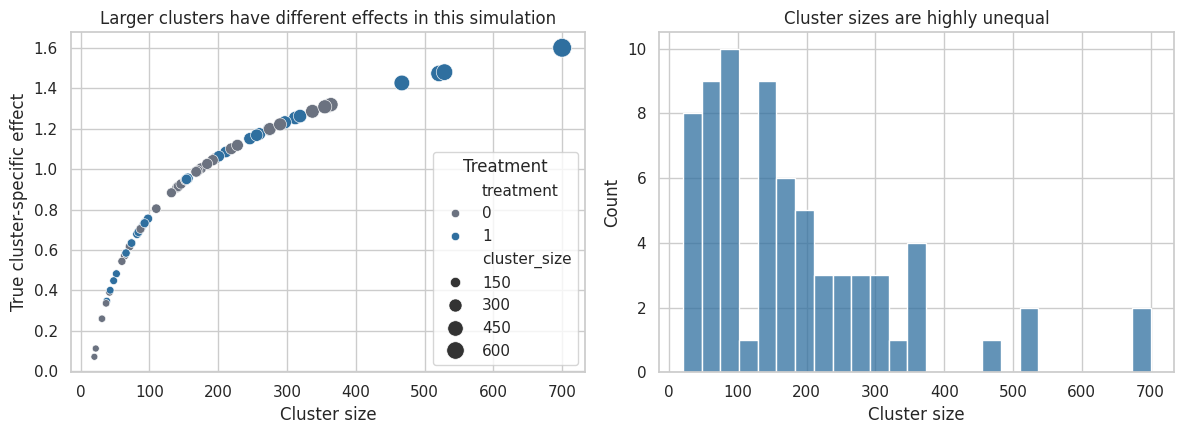

Interpretation

The true user-weighted and cluster-weighted effects differ because larger clusters have different treatment effects. That may happen in real business settings: large enterprise accounts may respond differently from small accounts, high-volume stores may respond differently from low-volume stores, and dense cities may respond differently from rural markets.

This is not a nuisance detail. It is a product question. If the decision is about total customer impact, user-weighted may be appropriate. If the decision is about whether the intervention works for a typical site, cluster-weighted may be appropriate. The analysis should match the decision.

9. Blocking and Pair Matching at the Cluster Level

Cluster randomization can produce imbalance when there are not many clusters. A simple improvement is to block or pair clusters using pre-treatment information, then randomize within each block or pair.

For example:

• Pair stores with similar pre-period sales, then randomize one store in each pair.
• Stratify regions by size and geography, then randomize within strata.
• Pair enterprise accounts by industry, contract size, and baseline usage.

Imai, King, and Nall (2009) argue that pair matching can recover efficiency in cluster-randomized experiments when feasible. The basic business intuition is simple: compare treated and control clusters that looked similar before treatment.

def assign_complete_randomization(clusters, seed=None):
    local_rng = np.random.default_rng(seed)
    n = len(clusters)
    treated = local_rng.choice(clusters.index.to_numpy(), size=n // 2, replace=False)
    z = pd.Series(0, index=clusters.index)
    z.loc[treated] = 1
    return z


def assign_pair_matched(clusters, match_col, seed=None):
    local_rng = np.random.default_rng(seed)
    ordered = clusters.sort_values(match_col).copy()
    z = pd.Series(0, index=clusters.index)
    for start in range(0, len(ordered) - 1, 2):
        pair_idx = ordered.index[start:start + 2].to_numpy()
        treated_idx = local_rng.choice(pair_idx, size=1)[0]
        z.loc[treated_idx] = 1
    if len(ordered) % 2 == 1:
        z.loc[ordered.index[-1]] = local_rng.integers(0, 2)
    return z


def standardized_difference(x, z):
    treated = x[z == 1]
    control = x[z == 0]
    pooled_sd = np.sqrt((treated.var(ddof=1) + control.var(ddof=1)) / 2)
    return (treated.mean() - control.mean()) / pooled_sd

local_rng = np.random.default_rng(20260430)
cluster_plan = pd.DataFrame({
    "cluster_id": np.arange(50),
    "pre_period_sales": local_rng.lognormal(mean=10.2, sigma=0.55, size=50),
})

balance_rows = []
for sim in range(1500):
    z_complete = assign_complete_randomization(cluster_plan, seed=sim)
    z_pair = assign_pair_matched(cluster_plan, "pre_period_sales", seed=sim)
    balance_rows.append({
        "method": "Complete randomization",
        "abs_standardized_difference": abs(standardized_difference(cluster_plan["pre_period_sales"], z_complete)),
    })
    balance_rows.append({
        "method": "Pair-matched randomization",
        "abs_standardized_difference": abs(standardized_difference(cluster_plan["pre_period_sales"], z_pair)),
    })

balance_df = pd.DataFrame(balance_rows)
balance_df.groupby("method")["abs_standardized_difference"].describe(percentiles=[0.5, 0.8, 0.9, 0.95]).round(3)

	count	mean	std	min	50%	80%	90%	95%	max
method
Complete randomization	1500.0	0.230	0.168	0.0	0.198	0.369	0.457	0.554	0.975
Pair-matched randomization	1500.0	0.052	0.035	0.0	0.049	0.088	0.095	0.101	0.123

fig, ax = plt.subplots(figsize=(9, 4.8))
sns.kdeplot(
    data=balance_df,
    x="abs_standardized_difference",
    hue="method",
    fill=True,
    common_norm=False,
    alpha=0.35,
    palette=["#b23b3b", "#2f6f9f"],
    ax=ax,
)
ax.set_title("Pair matching improves pre-treatment balance across clusters")
ax.set_xlabel("Absolute standardized difference in pre-period sales")
ax.set_ylabel("Density")
plt.tight_layout()
plt.show()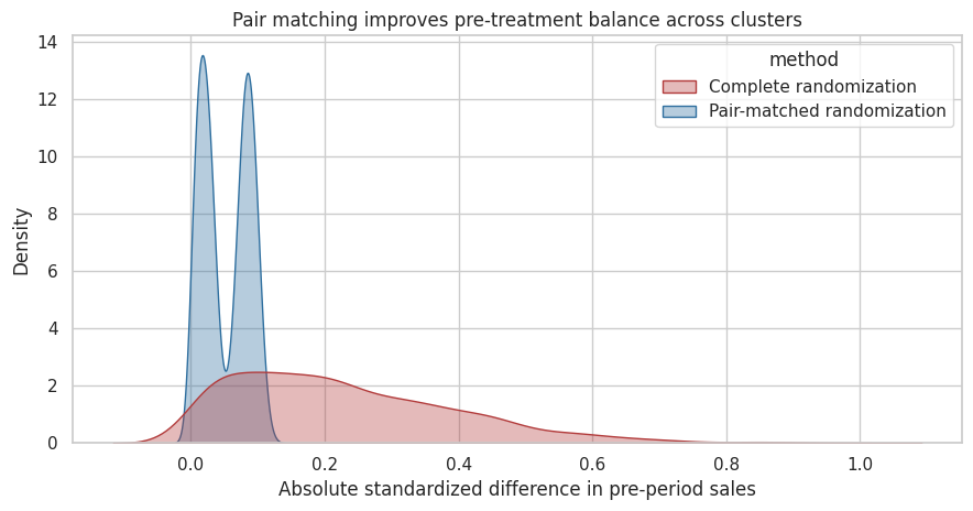

Interpretation

Pair matching sharply reduces the chance that treated clusters have much higher or lower pre-period sales than control clusters. This does not guarantee perfect precision, and the analysis should respect the matched design, but it is often a major improvement when clusters are scarce and heterogeneous.

For industry experiments, matching variables should be chosen before randomization and should be pre-treatment variables: baseline volume, geography, business segment, historical outcome level, device class, or platform role.

10. Choosing an Analysis Strategy

There is no single analysis rule for every clustered experiment. A useful workflow is:

Situation	Reasonable starting point
Many clusters, individual-level covariates matter	Individual-level regression with cluster-robust standard errors
Few clusters	Cluster-level analysis, randomization inference, or small-sample methods
Matched or blocked design	Include block indicators or analyze within matched pairs
Unequal cluster sizes	State cluster-weighted vs user-weighted estimand before analysis
Strong baseline predictors	Adjust for pre-treatment cluster-level or unit-level covariates
Spillovers across clusters	Reconsider cluster definition; may need network/interference design
Treatment delivered at cluster level but outcome at user level	Keep user-level metric definition, cluster-aware inference

A good analysis plan says what the randomization unit is, what the estimand is, and how uncertainty will be computed. It should be written before outcomes are inspected.

analysis_edges = [
    ("Business intervention", "Randomization unit"),
    ("Randomization unit", "Cluster assignment"),
    ("Cluster assignment", "Observed outcomes"),
    ("Observed outcomes", "Metric definition"),
    ("Metric definition", "Estimand"),
    ("Estimand", "Analysis method"),
    ("Randomization unit", "Analysis method"),
    ("Analysis method", "Decision readout"),
    ("Guardrails", "Decision readout"),
]
analysis_colors = {
    "Business intervention": COLORS["decision"],
    "Randomization unit": COLORS["cluster"],
    "Cluster assignment": COLORS["assignment"],
    "Observed outcomes": COLORS["outcome"],
    "Metric definition": COLORS["analysis"],
    "Estimand": COLORS["warning"],
    "Analysis method": COLORS["analysis"],
    "Decision readout": COLORS["decision"],
    "Guardrails": COLORS["warning"],
}

display(make_dag(analysis_edges, "Clustered experiment planning logic", analysis_colors))

11. A Clustered Experiment Planning Card

Here is a compact planning card for the retail example.

planning_card = pd.DataFrame({
    "field": [
        "Decision",
        "Intervention",
        "Randomization unit",
        "Observation unit",
        "Primary estimand",
        "Primary metric",
        "Expected ICC",
        "Cluster count",
        "Average cluster size",
        "Analysis plan",
        "Balance plan",
        "Guardrails",
        "Main risk",
    ],
    "example": [
        "Roll out merchandising policy to all stores?",
        "Store-level merchandising and staff checklist",
        "Store",
        "Customer visit",
        "User-weighted effect on customer value per visit",
        "Experiment-period customer value",
        "Use historical store data to estimate ICC before launch",
        "80 stores, 40 treatment and 40 control",
        "About 90 eligible visits per store",
        "User-level regression with store-clustered SE; cluster-mean sensitivity check",
        "Pair stores by pre-period sales before randomization if feasible",
        "Refunds, stockouts, support contacts, checkout latency",
        "Too few stores or large store-size imbalance",
    ],
})
planning_card

	field	example
0	Decision	Roll out merchandising policy to all stores?
1	Intervention	Store-level merchandising and staff checklist
2	Randomization unit	Store
3	Observation unit	Customer visit
4	Primary estimand	User-weighted effect on customer value per visit
5	Primary metric	Experiment-period customer value
6	Expected ICC	Use historical store data to estimate ICC befo...
7	Cluster count	80 stores, 40 treatment and 40 control
8	Average cluster size	About 90 eligible visits per store
9	Analysis plan	User-level regression with store-clustered SE;...
10	Balance plan	Pair stores by pre-period sales before randomi...
11	Guardrails	Refunds, stockouts, support contacts, checkout...
12	Main risk	Too few stores or large store-size imbalance

12. Key Takeaways

• Clustered experiments randomize groups, not individual rows.
• The unit of randomization drives the independence structure of the evidence.
• Positive ICC means rows inside the same cluster provide partially redundant information.
• The design effect, \(1 + (m - 1)\rho\), explains why large clustered datasets can have much smaller effective sample sizes.
• Naive user-level standard errors are often too small when treatment is assigned at the cluster level.
• Cluster-robust standard errors and cluster-level analyses are two useful ways to respect the design.
• Few clusters require special care; large-sample cluster-robust approximations may be fragile.
• Unequal cluster sizes force an estimand choice: average cluster or average user.
• Blocking and pair matching can improve balance and precision when clusters are scarce.
• A professional experiment plan names the randomization unit, estimand, ICC assumptions, analysis method, and guardrails before launch.

The next notebook will focus on noncompliance, intent-to-treat, and treatment-on-treated: what happens when assignment and actual treatment receipt differ.

References

Campbell, M. K., Elbourne, D. R., & Altman, D. G. (2004). CONSORT statement: Extension to cluster randomised trials. BMJ, 328(7441), 702-708. https://doi.org/10.1136/bmj.328.7441.702

Cameron, A. C., & Miller, D. L. (2015). A practitioner’s guide to cluster-robust inference. Journal of Human Resources, 50(2), 317-372. https://doi.org/10.3368/jhr.50.2.317

Desai, M., Bryson, S. W., & Robinson, T. N. (2013). On the use of robust estimators for standard errors in the presence of clustering when clustering membership is misspecified. Contemporary Clinical Trials, 34(2), 248-256. https://doi.org/10.1016/j.cct.2012.11.006

Handlos, L. N., Chakraborty, H., Sen, P. K., & Sammel, M. D. (2009). Evaluation of cluster-randomized trials on maternal and child health research in developing countries. Tropical Medicine & International Health, 14(8), 947-956. https://doi.org/10.1111/j.1365-3156.2009.02313.x

Imai, K., King, G., & Nall, C. (2009). The essential role of pair matching in cluster-randomized experiments, with application to the Mexican Universal Health Insurance Evaluation. Statistical Science, 24(1), 29-53. https://doi.org/10.1214/08-sts274

Kennedy-Shaffer, L., & Hughes, M. D. (2021). Power and sample size calculations for cluster randomized trials with binary outcomes when intracluster correlation coefficients vary by treatment arm. Clinical Trials, 19(1), 42-51. https://doi.org/10.1177/17407745211059845

Peerawaranun, P., Landier, J., Nosten, F. H., & Chaumeau, V. (2019). Intracluster correlation coefficients in the Greater Mekong Subregion for sample size calculations of cluster randomized malaria trials. Malaria Journal, 18, 428. https://doi.org/10.1186/s12936-019-3062-x

Taljaard, M., Teerenstra, S., Ivers, N., & Fergusson, D. A. (2016). Substantial risks associated with few clusters in cluster randomized and stepped wedge designs. Clinical Trials, 13(4), 459-463. https://doi.org/10.1177/1740774516634316